Publisher’s version / Version de l'éditeur:
ASHRAE Transactions, 100, 2, pp. 1251-1263, 1994
READ THESE TERMS AND CONDITIONS CAREFULLY BEFORE USING THIS WEBSITE.
https://nrc-publications.canada.ca/eng/copyright
Vous avez des questions? Nous pouvons vous aider. Pour communiquer directement avec un auteur, consultez la
première page de la revue dans laquelle son article a été publié afin de trouver ses coordonnées. Si vous n’arrivez pas à les repérer, communiquez avec nous à PublicationsArchive-ArchivesPublications@nrc-cnrc.gc.ca.
Questions? Contact the NRC Publications Archive team at
PublicationsArchive-ArchivesPublications@nrc-cnrc.gc.ca. If you wish to email the authors directly, please see the first page of the publication for their contact information.
NRC Publications Archive
Archives des publications du CNRC
This publication could be one of several versions: author’s original, accepted manuscript or the publisher’s version. / La version de cette publication peut être l’une des suivantes : la version prépublication de l’auteur, la version acceptée du manuscrit ou la version de l’éditeur.
Access and use of this website and the material on it are subject to the Terms and Conditions set forth at
Air change rates and carbon dioxide concentrations in a high-rise
office building
Reardon, J. T.; Shaw, C. Y.; Vaculik, F.
https://publications-cnrc.canada.ca/fra/droits
L’accès à ce site Web et l’utilisation de son contenu sont assujettis aux conditions présentées dans le site LISEZ CES CONDITIONS ATTENTIVEMENT AVANT D’UTILISER CE SITE WEB.
NRC Publications Record / Notice d'Archives des publications de CNRC:
https://nrc-publications.canada.ca/eng/view/object/?id=f6f2cf7d-0a57-4a85-946f-cd6cfe3a28c9 https://publications-cnrc.canada.ca/fra/voir/objet/?id=f6f2cf7d-0a57-4a85-946f-cd6cfe3a28c9Air c ha nge ra t e s a nd c a rbon diox ide c onc e nt ra t ions in a high-rise
offic e building,
N R C C - 3 5 9 8 7
R e a r d o n , J . T . ; S h a w , C . Y . ; V a c u l i k , F .
J a n u a r y 1 9 9 3
A version of this document is published in / Une version de ce document se trouve dans:
ASHRAE Transactions, 100, (2), ASHRAE Annual Meeting, Denver, CO, USA,
93, pp. 1251-1263, 94
http://www.nrc-cnrc.gc.ca/irc
The material in this document is covered by the provisions of the Copyright Act, by Canadian laws, policies, regulations and international agreements. Such provisions serve to identify the information source and, in specific instances, to prohibit reproduction of materials without written permission. For more information visit http://laws.justice.gc.ca/en/showtdm/cs/C-42
Les renseignements dans ce document sont protégés par la Loi sur le droit d'auteur, par les lois, les politiques et les règlements du Canada et des accords internationaux. Ces dispositions permettent d'identifier la source de l'information et, dans certains cas, d'interdire la copie de documents sans permission écrite. Pour obtenir de plus amples renseignements : http://lois.justice.gc.ca/fr/showtdm/cs/C-42
OR-94-22-1
AIR CHANGE RATES AND CARBON
DIOXIDE CONCENTRATIONS IN A
HIGH-RISE OFFICE BUILDING
James T. Reardon, Ph.D.
Chia-yu Shaw, Ph.D., P.Eng.
Member ASHRAE
Frank Vaculik, P.Eng.
Member ASHRAE
ABSTRACT
The feasibility of controlling ventilation rates using occupant-generated carbon dioxide (C02) as the control index has been examined in a large high-rise office building with a constant-volume heating, ventilating, and air-condi-tioning (HVAC) system. Daily C02 concentration profiles throughout the building and air change rates, using sulfur hexafluoride (SF6) as a tracer gas, were measured for several outdoor air supply rates. Of particular interest was how well the C02 concentrations measured in the central ventilation system's return air plenum represented the average C02 concentration behavior in the building as a whole. C02 concentration profiles were also measured on individualjloorspaces in the building to determine the range of variability in the concentration behavior in occupied zones. The influence of fresh air supply rates on the speed of mixing of the tracer gas (surrogate contaminant) was also examined. The practicability of using C02 as an active
tracer gas to measure air change rates was also
investigat-ed. The results are discussed in the paper.
INTRODUCTION
As the public, and the general work force in particular,
has become more aware of air quality issues in recent years,
building operators have faced increasing pressures to ensure that air quality in workplaces is acceptable in terms of both health and comfort. While some indoor spaces may be inadequately ventilated and experiencing air quality prob-lems, other seldom-used indoor spaces, such as meeting rooms and auditoriums, may be overventilated and thus wasting energy. Ventilation system control based on C02 concentration has been proposed as a means to help save energy in these spaces during periods of low or no occupan-cy (Vaculik 1987). In addition, C02-based ventilation control may also offer a means of directly solving some indoor air quality problems by increasing ventilation air supply rates to areas of high demand (Woods et al. 1982).
Some research has been done to examine the use of occupant-generated C02 as an active tracer gas for measur-ing buildmeasur-ing air change rates (Smith 1988; Turiel and Rudy 1982; Turner et al. 1985). Some benefits of this approach are that no additional pollutants (tracer gases) need to be introduced into the indoor environment, occupant-generated C02 is freely available, and its sources are typically distrib-uted throughout a building, thus leading to good mixing. Many of the problems inherent in this approach have been described by others who have tried to use it (Persily and Dols 1989). What has not been fully explored is the ques-tion of how well this technique might work as a practical measurement tool, despite its fundamental and theoretical sources of uncertainty. One major issue is that, while occu-pant-generated C02 levels may not be used to measure the total building air change rate because fundamental as-sumptions are violated, the technique may measure how well the occupants' needs for ventilation are being met.
The study reported in this paper was carried out with two major objectives. The first was to evaluate the potential for C02-based demand control of the constant-volume ventilation system in the test building. The second objective was to evaluate the practical feasibility of using the decay of occupant-generated C02 as an active tracer gas to measure the air change rates in the test building.
MEASUREMENT APPROACH Test Building
The test building is a 22-story office building with a total interior volume of approximately 113,700 m3 (4,012,200 ft3) and approximately 37,900 m2 (408,000 ft2)
total floor area. It is located in Ottawa and is surrounded by many lower buildings in a fairly open terrain. The 22nd floor houses all the HV AC equipment. There are seven all-air consiimt-volume supply all-air-handling systems and two return air-handling systems. Four core supply systems provide air to the east and west interior lower zones (floors
James T. Reardon is a research officer and Chia-yu Shaw is a senior research officer at the Institute for Research in Construction,
National Research Council of Canada, Ottawa, ON. Frank Vaculik is manager of the Building Performance Division, Architectural and Engineering Services Branch, Public Works Canada, Ottawa, ON.
ASH RAE Transactions: Symposia 1251
I
•
2 through 11) and the east and west interior upper zones (floors 12 through 21). Three supply induction systems pro-vide air to the south perimeter, east and east half of the north perimeter, and west and west half of the no.rth perimeter zones, which each include floors 2 through 21. The two return systems draw air from the east and west halves of the entire building. There are independent supply and exhaust systems for the first floor, which includes the entrance lobbies and a large cafeteria. Constant-volume exhaust systems continually exhaust air from the
wash-rooms.
The components of a C02-based demand controller for the ventilation systems' outdoor air (OA) supply are installed in the building. The C02 sensors are located inside the tops of the two return air shafts and are connected to provide the average of their readings to the central control system.
Equipment Setup
Instrumentation An automated data-acquisition system was installed for the SF6 tracer gas measurements and automatic monitoring of C02 concentrations throughout the building. The instrumentation and data-acquisition equip-ment were functionally identical to that used by Shaw et al. (1991). C02 concentration measurements (in the range of 300 to 2,500 ppm) were accurate to ±I% f.s.d. (±25 ppm). SF6 tracer gas concentration measurements (in the range of I to 200 ppb) were accurate to ±I% f.s.d. (±2 ppb). The time required by each instrument to analyze a sample was 15 seconds, allowing a sampling rate of four per minute.
Sample Tubing Network Air samples were drawn through a network of tubes from various locations through-out the building by diaphragm pumps with flow rates of 2.5
Umin
(5.29 ft3/h). This ensured that fresh samples were immediately available when selected by the 16-position sampling valve. In addition to being able to analyze gas samples from each sample line individually, airflows from any combination of sampling locations could also be directed into a small manifold chamber, where they mixed. This arrangement provided a tracer gas sample representing spatially averaged air from all the sampling locations connected to the manifold for continuous monitoring ofthe building's air change rate. Further details of an identical system can be found in Shaw et al. (1991).Sampling Locations Floors 2, 5, 8, II, 12, 15, 18, and 20 were selected as the test floors. Sample lines connected the pumps to the openings of the east and west return air shafts in the ceiling plenums of each test floor. In addition, sampling lines were connected to one position each in the occupied zone of test floors 2, 5, 8, II, 18, and 20. Two sample lines were connected to sampling locations at the top of the east and west return air shafts, and another sample line led to the roof to allow the outdoor air to be sampled. Several different combinations of sample lines were con-nected to the sampling valve and manifold for different types of tests.
1252
Test Procedures
The three types of measurements carried out in the work reported herein were (I) air change rate measurements, (2) air distribution measurements, and (3) C02 concentration
monitoring.
Air Change Rate Measurements The initial series of air change rate measurements was conducted to determine the relationship between the ventilation systems' outdoor air damper settings and the air change rate. The building's air change rates were measured at the following outdoor air damper settings: 100%, 75%, 50%, 35%, and 20%. The 20% outdoor air damper position was the minimum setting used by the building operations staff. These so-called percentages of outdoor air are simply labels for the damper positions as set by the HV AC systems' computerized controls; they do not imply that the actual percentage of outdoor air in the supply airstream was measured.
The air change tests were carried out using the tracer gas decay method. SF6 gas was introduced evenly, in small amounts, into the building's ventilation supply airstreams at the start of each test and allowed to decay. The initial series of air change rate tests used a combination of automatic and
manual sampling to measure the tracer gas concentrations
ai
individual locations throughout the building. Later tests used the manifold technique to measure spatially averaged whole-building air change rates.
Air Distribution Measurements The air distribution tests served to verify that the ventilation system adequately distributed the outdoor air supply to all occupied areas in the building. They served to verify that the air in the building was sufficiently well mixed to allow the tracer gas decay method to provide accurate measurements of the air change rates. The air distribution tests also used tracer gas decay methods. The tracer gas was released into only one of the four interior-zone supply air ducts to create a temporary "source zone" of contamination in the building and thereby pose a challenge for the air distribution system.
Carbon Dioxide Concentration Monitoring Carbon dioxide concentrations outdoors and at the various locations in the building (according to the sampling system's configu-ration) were monitored continuously, 24 hours a day, by the automated data-acquisition system. The C02 concentrations outdoors were monitored continuously to provide the background concentration in the outdoor air brought into the building by the ventilation system. Ventilation system settings of 100%, 75%, 50%, 35%, and 20% (minimum) of outdoor air were used for these tests.
MEASURED RESULTS
To evaluate the potential for C02-based, demand-controlled ventilation, it is necessary to know where to lo-cate the C02 sensor and the relationship between the air change rate and C02 concentrations at the sensor location as well as in the occupied zones. Test results affecting these issues will be discussed.
Air Distribution Patterns and Mixing Times
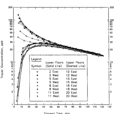
The results from a typical early air distribution test-at 20% outdoor air damper settings, where the tracer gas was injected only into the west interior upper (WIU) supply
shaft-are shown in Figures 1 and 2. The data in Figure l
clearly demonstrate the typical source zone and target zone concentration behaviors: pure decay in the upper zone and an initial increase followed by decay in the lower zone. Some of the east locations on the upper floors demonstrate a target zone behavior, with lower concentrations at the earlier times. These return air data suggest that adequate mixing in the building is achieved after approximately 70 minutes following unbalanced injection. Figure 2 shows the results on a typical source-zone floor (the 20th). These results demonstrate some local source (west and center) and target (east) zone behavior on a single floor and suggest that mixing on the floor space is only complete about 80 minutes following injection.
The results of a typical air change rate measurement, where tracer gas was injected uniformly into all four interior supply systems, are plotted in Figure 3. They suggest that mixing was complete soon after injection. This test was carried out with the outdoor air dampers set to 20%. The air change rate was measured to be 0.6 air changes per hour (ach). Results from data from individual floors indicated that the mixing improves with height in the building, i.e., upper floors are progressively better mixed than lower floors. This is probably due in part to the fact that all the fans of the mechanical system are located on the 22nd floor. Conse-quently, longer ducts with greater losses result in less vigorous airflows being delivered to the lower floors and poorer mechanical mixing. Therefore, even though the data measured in the openings of the return air shaft suggest complete mixing as soon as 20 minutes after a balanced injection, only concentration data measured 60 minutes following injection were used for all air change rate calcula-tions.
To test whether higher outdoor air supply rates, and consequently reduced recirculation rates, might slow the mixing within the building, additional air distribution tests were carried out with outdoor air damper settings of 50%, 75%, and 100%. Figure 4 shows the results of a test at 50% OA, where the tracer gas was injected into the east interior upper supply shaft. These data suggest that mixing was complete in ihe building by 80 minutes after injection. Other tests at 50% OA using the other three interior supply shafts individually as injection sites also demonstrated complete mixing by 80 minutes after injection. The test results at 75% and I 00% OA also confirm that mixing was complete by 80 minutes after an unbalanced injection of tracer gas. Collec-tively, these re;ults suggest that mixing in the building does not depend on the amounts of outdoor and recirculated air in the supply airstream. The inference is that mechanical recirculation is not the principal mixing process in the building. Instead, interzonal airflows through penetrations
ASH RAE Transactions: Symposia
•
u ;E 200 Qセ@"
"
"
50"
' '
'
6'
'
'
'
'
'·
'
セMMセᄋ\[@'·
..•
··'<>-. ····o. .... セZMMMZセZNGZ@ ......
セ@
Legend: Lower FloorsSymbol (Solid Line)
0 2 East
•
2 West.
.
5 East 5 West 0 8 East.
8 West•
11 East•
11 West...
Upper Floors (Dashed Line) 12 East 12 West 15 East 15 West 18 East 18 West 20 East 20 West'
'
' '
'
6go
0 0 0 0 0'
'
'
0'
0'
'
0' '
6'
10 20 Jo 40 50 so 70 ao 90 100 110 120 1JoElapsed Time, min
Figure I Air distribution test results from automated
sampling of return air plenums at 20% OA--west interior upper injection site.
"'
""
'""
60 60'"
60 60 20"
60 60 60 60'"
'"
D"
30 セ@ セ@ o" 20"
0 セ@ 1'•
Legend: g'"
'"
0'
'
u'
'
•
'
Symbol Sampling Location'
6 6
u
West Return Air
;E
'
East Return AirNW Floor (A) NE Floor (B) Centre Floor (C) SW Floor (D) SE Floor (E)
'
0 10 20 JO 40 50 GO 70 SO SO 100 t 10 \20 130'
Elapsed Time, min
Figure 2 Air distribution test results measured on the
20th floor, automated and manual sampling at
20% OA-west interior upper injection site.
and interconnections such as elevator and utility shafts, driven by unbalanced supply and return airflows and other factors (such as the pumping effect of moving elevator cars), must play a major role in whole-building mixing. The previous findings at 20% OA suggested that mixing with balanced injection of the tracer gas dose is much faster than with deliberately unbalanced injection. Therefore, a mixing
1253
·--
" ,' ' • '" セ@ " セ@ < ' ' ;,, ANIセセ^@ セ@ セセLNLMMセMセMMセ@ ",! '
il
200 Gセ@80
"
60 50"
JO 20"
' '
' '
5 2'
2 qMセ@
'
:I
' '
'
'
'
'
5•
セ@ 2 Legend:Lower Floors Upper Floors
'
Symbol (Solid Line) (Dashed Line)
'
0 i2 East 12 East
•
2 West 12 West.
5 East 15 East.
5 West 15 West 0 8 East 18 East.
8 West 18 West 0 1 t East 20 East•
11 West 20 West'
10 20 JO 40 so 50 10 eo 90 100 no 120 1JOElapsed Time, min
go
0 0 0 0 0 0Figure 3 Tracer gas mixing test results measured with automated sampling at minimum (20%) out-door air damper setting for balanced injection.
time allowance of 60 minutes was deemed appropriate for tracer gas measurements of air change rates for the full range of outdoor air damper settings.
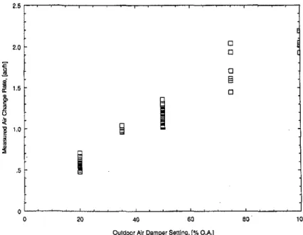
Relationship between Air Change Rate and Outdoor Air Damper Settings
All the measured air change rate data are plotted with their corresponding damper settings in Figure 5. The results indicate that a linear relationship exists between the two. The average air change rates delivered when the ventilation system was set to provide 20% and I 00% outdoor air were approximately 0.58 and 2.1 ach, respectively (the values ranged from 0.45 to 0. 76 ach for the 20% setting and from
1.9 to 2.4 ach for the I 00% setting). ·
The supply air damper settings are not the only factor affecting the building air change rate. The HV AC system's exhaust air dampers are designed as pressure relief vents; therefore, their action will affect the overall air change rate in the building "set" by the supply air dampers. Due to their design, the position of the exhaust air dampers could not be fixed or monitored automatically. However, the magnitude of this effect is expected to increase with the outdoor air supply rate and may account for the generally greater scatter observed in the data for higher OA damper settings.
Carbon Dioxide Patterns
Daily Concentration Profiles Typical C02
concentra-tion profiles for a midweek working day, at the minimum (20%) outdoor air supply, are shown in Figures 6a and 6b. Figure 6a shows concentrations measured at locations in the
1254
JOO
lOo
200 Test West East Floor
Floor Return Return Space 200
2 0 0 5
•
•
'!8 8 D•
D 180"
70 11 0 0"
60 12•
10..
"
15•
•
"
D"
18•
•
..
•
•
"
20•
•
c Line: Solid Do shed JO
0 Dotted ·; 20 セ@0
"'
•
0 0J
0'S
!0 u•
0'
'
I
'
1 E: d
•
セ@'
•
Ll⦅セlMMMlMMMセMMセMMセMMセMMセMMセ@ 0 JO 60 90 120 150 180 210 セTP@Elapsed Time, min
Figure 4 Air distribution test results measured by the automated sampling system at 50% OA-easr interior upper injection site.
occupied zones of floors 2, 8, II, 18, and 20, and outdoors. Figure 6b shows concentrations measured at the openings of the return air shafts on the same test floors. Each profile peaks at noon, declines slightly over the lunch hour, and peaks at a higher concentration at the end of the workday (approximately 4 p.m.). Typical results of more spatially detailed sampling for the same day as shown in Figure 6 are shown in Figures 7a and 7b. Figure 7a compares the manually sampled results in the occupied zone of the second floor with measurements from the openings of the second floor's return air shafts. Figure 7b compares the results of automated monitoring in the occupied zone of the 18th floor with measurements from the openings of that floor's return air shafts.
These results indicate that on all the test floors, the C02 concentrations measured in the occupied floorspace are more variable than data measured in the openings of the return air shafts on the same floors. This was expected, since the air entering the return air shafts is drawn together from the entire floor through the ceiling plenum and should represent a spatial average of the particular floor. Figure 7b suggests that the concentration profile of return air C02 fairly well
represents the average of the C02 concentration data
measured in the occupied zone during the working day
(period of heavy occupancy). However, the floorspace 、。セ@
are valued slightly but consistently higher than the return wr data during unoccupied periods of the day. This suggests some degree of short-circuiting in the building's ventilation. i.e., some ventilation supply air found its way into the return air shafts before it had mixed with the air in the occupied floors pace.
ASH RAE Transactions: Symposia
2.5 2.0 0 0
I
0t
§ セ@ 1.5 0•
セ@ セ@ u セ@ セ@ 1.0 セ@ セ@ .5Outdoor A!r Damper Setting,[% O.A.]
Figure 5 Measured air change rates plotted with corresponding outdoor air damper positions.
1000 900
---
2F ··· SF·-··-··-··-··-"
---
11F 600---
18F'
e
··· 20F セ@ ii_--: セ@•
700 !'rA" \
セセMZMNA@
vr*'
セM
.'JᄋMMセ@
I
tLセN@
'i!'\'j{,:
セMG@ ,'.
/
··'
0 600 ug"
500l
400 300 0 4 6 12 16 20 24 Time of Day, [h)Figure 6a Typical weekday floorspace C02 concentration profiles for minimum (20%) outdoor air supply.
This short-circuiting may be responsible, in part, for the apparently larger discrepancies observed in Figure ?a, which are typical of all the test floors (2, 5, 8, II, 12, and 15) on which manual sampling was carried out. However, another possible contributing factor was that the manual samples were measured at normal standing nose height (approximate-ly 1.5 m [5 ft] above the floor) in walkways, aisles, and the centers of offices and reception areas. These locations were hence much closer to the influence of occupants' breathing (and therefore might be expected to yield higher C02 concentrations) than the sample locations used by the automated system, which were typically located on walls
ASH RAE Transactions: Symposia
and electrical poles at heights of approximately 2.1 m (7 ft). The data in Figure ?a were also measured on the lowest test floor, which, as noted earlier, tends to be less weU mixed than the upper floors.
Daily Average and Peak Concentrations The prototype C02-based demand controller has its sensors located at the tops of the two main return air shafts. The relationship between the C02 concentrations measurable at these sensor locations and the building's overaU C02
concentration was examined. The concentrations measured
at each sampling location were averaged over the principal working day-9 a.m. to 4 p.m. The concentrations measured
1000 900 aoo 'E セ@
t
700 g•
E § 600 8 o" <.> 500 400 300 0 ·••••••••••·• 2A .. -·-·- SA ·--- 8A 11R""
20R Outdoors 4 a 12 16 20 24 Time of Day, [hjFigure 6b Typical weekday return air C02 concentration profiles for minimum (20%) outdoor air supply.
1000 2nd Fleer Flcorspace 900 - - Return Plenum 0 8 セ@ 8
; I
''"
6 0 0•
I
0 ' I'
'
"
700 0a
2セ@
•
セ@
600 o" <.> 500 400 300 0 4•
12 16 20 24 Time of Day, (h)Figure 7a Comparison of C02 concentrations measured in the jloorspace and return air on the second floor-minimum
(20%) outdoor air.
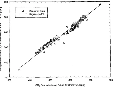
in the return air shaft openings on each of the eight test floors were averaged for each day and compared to the daily average concentrations measured at the tops of the two return air shafts. The results are shown in Figure 8 along with the zero-intercept regression line fitting the data. The curve fit indicated that the average of the daily average concentrations of the individual return air levels is generally 1.5% higher than the daily average concentration at the shaft top. A similar.comparison of the concentration at the return air shaft top with the average of daily average
concentra-1256
tions measured in the occupied floorspaces is shown in Figure 9. The linear regression analysis indicates that the
daily average concentrations from the shaft top must セ@
increased by 3.6% to represent the average of the datly
average concentrations in the occupied zones. These results
indicate that the measurement location at the return air shall top well represents the behavior for the entire building.
The daily maximum C02 concentrations ュ・。ウオセ@ at
the tops of the return air shafts were also compared wtth the daily average of the maximum or peak concentrations
ASHRAE Transactions: Symposia
Fig1. rnea::-. pied セッョウ@ How, セNZッョ」ャ@ rcpre \Uggt locati, I cr. T the dt <lir sh o\SH
d
---1000 900 18th Floor Floorspace 0 - - Retum Plenum aoo 0
e
セ@"
7001
8
600 o" u 500 400 300 0 4 6 12 16 20 24 nme of Day, {h]Figure 7b Comparison of C02 concentrations measured in thejloorspace and return air on the 18th floor-minimum (20%)
outdoor air.
aoo
0
e
セ@ 0
セ@
700 Measured Data Regression Fitセ@
:; 600 0 0.•
€
•
0 0 0"
o" 500 0"
セ@ §•
"'
•
400セ@
セ@ 300 300 400 500 600 700 600C02 Concentration at Return Air Shaft Top, [ppm}
Figure 8 Comparison of daily average C02 concentrations measured at the tops of the return air shafts and the average of daily average concentrations at the test floors' return air shaft openings.
measured at the return air shaft openings and in the occu-pied zones on each test floor. As expected, these compari-sons displayed a poorer correlation and more scatter. However, the general conclusions are the same-that the concentrations measured at the return air shaft top well represent the concentrations throughout the building. This suggests that the return air shaft top is an appropriate location for the C02 sensor of a ventilation demand control-ler.
These findings provide support for the idea of locating the demand· controller's sensor(s) in the top(s) of the return air shaft(s) if whole-building demand is to be the basis of
ASH RAE Transactions: Symposia
ventilation system control. However, the setpoint of the demand controller must account for the differences observed between the C02 concentrations measured in the occupied floorspace areas and at the top(s) of the return air shaft(s). Relationship between C02 Concentrations
and Air Change Rate
The next issue of interest was the relationship between air change rate and a representative C02 concentration. One simplified analytical approach to predict daily peak C02
concentrations is based on the constant-injection tracer gas
1257
-800 'E .@; 0 Measured Data
セ@
700 Regression Fitセ@
0 0 0 600セ@
•
セ@ 0 0 8g'
500 Bセ@
0 0 セ@•
セ@ 400•
•
セ@ 300 300 400 500 600 700 800C02 Concentration at Return Air Shaft Top, [ppm]
Figure 9 Comparison of daily average C02 concentrations measured at the tops of the return air shafts and the average of daily average concentrations in the occupied zones of the test floors.
method. Shaw (1988) found good agreement between predictions based on steady-state constant-injection and measured daily peak concentrations. This was somewhat surprising because fundamental assumptions of constant source strength and air change rate for sustained periods of occupancy are not strictly valid in most office buildings (Persily and Dols 1989). The equation used by Shaw is
where
cmax
=
co
=
G=
1=
N=
v
=
Cmax = [(G·N)/(/·V)] ·(360011000) ·(106)+co
(I)maximum C02 concentration in the occupied
space (ppm),
C02 concentration in outdoor air (ppm),
C02 generation rate per person (Us),
air change rate (ach), number of occupants, and building volume (m3).
In this building, the normal number of occupants is 1,100
and the C02 concentration in outdoor air is typically 350
ppm. The building volume is approximately 113,700 m3 (4,012,200 ft3). ASHRAE Standard 62-1989 (ASHRAE 1989) recommends a default C02 generation rate per person
of 0.005 Us (0.0106 cfm) for office workers, corresponding
to an activity level of 1.2 met (light office work).
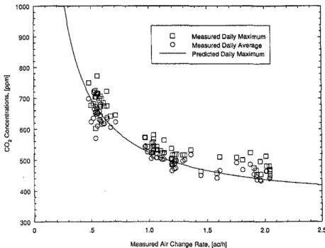
This equation was used to predict the daily peak C02 concentrations, and in Figure 10 the results are compared with data measured at the top of the return air shaft. The predictions agree best with . the measured daily average
1258
concentrations and therefore underestimate the daily peak concentrations slightly. Table 1 lists the ranges of daily peak
C02 concentrations measured in the individual returns and
occupied floorspaces and, for comparison, the predictions based on the average measured air change rates for each setting of the outdoor air dampers tested. The comparison supports the relationship's general validity for this building. The comparison is not so good for the 100% OA setting, perhaps due to the fact that fewer data are available for this condition. While it might be tempting to generalize, it must be noted that the exact relationship can be expected to be
building-specific, in that the parameters in Equation 1 will vary for different buildings and the validity of the as•ump-tions may not apply to all types of office buildings.
These results indicate that, as expected, as the air change rate and outdoor air supply rate increase, the C02 concentrations generally decrease, as illustrated by lower daily average and peak values. The results also indicate that the C02 concentrations measured in the return air shafts are generally slightly lower than those measured in the occupied floorspace. Therefore, if the smoother profiles that are measured in the return air shafts are to be used in a COz· based demand control strategy to represent the concentration in the whole building, the target setpoint concentration must be decreased by 10% (i.e., a correction factor of about 0.9 must be applied) to account for the somewhat higher concentrations in the occupied zones in this particular buil· ding.
It is also interesting to speculate as to why the predic-tions based on steady-state constant-emission theory agree so well with the measured data. Certainly, as pointed out by Persily and Dols (1989), the number of occupants will
ASH RAE Transactions: Symposia
-1000 900 800 'E セ@
""
セ@ Mセ@ 700 E セ@ 600 0 () o" () 500 400 300 0 0 a .5 1.00 Measured Daily Maximum 0 Measured Dally Average
Predic1ed Dally Maximum
1.5 2.0 2.5
Measured Alr Change Rate, [ac/hl
Figure 10 Comparison of predicted daily peak C02 concentration and measured daily average and peak concentrations at the top of the return air shaft.
TABLE 1
Peak C02 Concentrations-Ranges of Values
Outdoor Return Air Occupied Average Predicted
Air Shaft Openings Floorspaces Air Peak C02
Damper Minimum Maximum Minimum Maximum Change Concentration
Setting [% O.A.] [ppm] [ppm] [ppm] 20 564 866 575 35 498 593 489 50 450 645 491 75 420 550 483 100 441 570 466
fluctuate during a typical working day, as indicated by the typical daily C02 concentration profile. The good agreement suggests that in an office building of this size and popula-tion, the normal comings and goings of the occupants and the variations in their activity levels typically average together to produce a daily average and peak concentration equivalent to what would be produced by a constant population. Visitors during the working day probably help offset normal occupants who may be out of the building, and variations in activity levels (C02 generation rates) round out the balance. This effect may vary for other types of buildings and occupancies, such as educational institutions, health care facilities, and retail establishments.
Carbon Dioxide Decay Analysis
The second principal issue of interest in this study was to examine the suitability of using the decay in C02
ASH RAE Transactions: Symposia
'' i
ii
iii
[ppm] [aclh] [ppm] 951 0.58 650 624 0.99 526 708 1.21 494 634 1.69 453 624 2.10 433concentration at the end of the working day as an active tracer gas measurement of the building's air change rate. Persily and Dols (1989) have rejected this approach because several assumptions fundamental to the technique are not strictly valid. An attempt was made here because this method has been used in many other published studies.
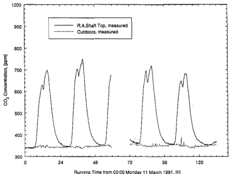
From all the data collected, the C02 concentrations measured during the week of March II to 16, 1991 (Mon-day to Satur(Mon-day), were selected. The concentrations mea-sured at the top of the return air shaft and outdoors are shown plotted in Figure II, with running time from mid-night Monday, March II, 1991. This data set offered an almost continuous record for a complete work week (Mon-day through Fri(Mon-day), with outdoor air dampers set at their
20% positions for 24-hour-per-day operation, for which daily air change rate measurements were available. Each day of this record offered a relatively clean end-of-day concen-tration decay. Records of occupants entering and leaving during most of the decay period were also available.
1000
900 R.A.Shaft Top, measured
Outdoors, measured 800
I
c 700 0 ᄋセ@•
セ@c 0 600"
o""
500 400 300 a 24 48 72 96 120Running Time from 00:00 Mor1day 1 1 March 1991, [hJ
Figure 11 C02 concentrations measured during the week of March ll-16, 1991, at the return air shaft top and outdoors-minimum (20%) outdoor air.
The mass balance equation describing the expected C02
concentration behavior is
dC!dt = -l·(C -C0) +S/V (2)
where
c
=
C02 concentration in the building (kg/m3),co
=
C02 concentration in outdoor air (kglm\t
=
time from the effective start of decay (h),I
=
building air change rate (ach),s =
internal C02 generation rate (kg/h), andv
=
building volume (m3).Assuming that no sources are present (S
=
0), the solution of this equation is the following:C = K·e(-l·t) +C
0 (3)
where K is the effective concentration difference between
indoors and outdoors at the effective start of the decay (K
= C- C0 at t = 0).
From the entry and exit records, it was clear that the test building always contained some occupants; therefore,
the assumption S = 0 was never strictly true. However,
simple decay analyses were performed to examine the influence of a nonzero source on the calculated decay rates.
For these calculations, the reference concentration C
0 was
the average of the measured outdoor concentration for the period of the decay, and an exponential curve was fitted to the measured concentration data for the overnight period following each working day. In Table 2, the results are compared with air change rates measured using the SF6 tracer gas decay techniques described previously.
1260
The curve-fit procedure involved selecting a section of the concentration profile that had a suitable shape and large
enough concentration differences (i.e., C- C0) to provide an
acceptable goodness-of-fit. The start and end times of the selected concentration data are also listed in Table 2, in decimal hours from midnight at the beginning of the first day of each two-day period. In four of the five days reported in Table 2, this section of decay began shortly after the nominal end of the working day at 4 p.m. (16.000 h) and ran until late evening or very early the following morning. These were Monday, Tuesday, Thursday, and Friday nights. The decay analysis for the Wednesday to Thursday overnight period starts just after midnight because
the C02 concentration data for the latter half of Wednesday
were not available due to an interruption in monitoring. The curve-fits for the four periods beginninll in the
afternoons resulted in goodness-of-fit parameter (r') values
greater than 0.99, and standard error estimates for the
calculated decay rates of less than 1.5%. The C02 decay
rate calculated for the Wednesday-to-Thursday period, using a later relative time period, resulted from a goodness-of-fit of
,2
= 0.50 and has a standard error estimate of 20.8%, obviously a much poorer quality result. The underestimationby the C02 decay technique of the SF6-measured air change
rates ranged from 20% to 36%, except for the later curve fit reported for the Friday-to-Saturday period, which was underestimated by 50%.
A comparison of the measured decay and the fitted exponential curve for two of the overnight periods is shown in Figures 12a and 12b. Figure 12a illustrates the two curve fits for the Tuesday evening decay period (March 12-13. 1991). While the two curves were fitted over different time periods, as indicated in Table 2, they are plotted for the total
TABLE 2
Comparison of Decay Rates from C02 and SF6 Tests
Date Decay Decay r" Std. Rei. Start End
Rate Rate Err. Error Time Time
(SF,) (C02 ) Est. (C02) (C02) [ac/h] [ac/h] [%] [%] (h] (h] 91/03/11-12 0.57 0.39 0.995 1.27 -31.6 16.211 25.344 91/03/12-13 0.48 0.36 0.994 1.16 -25.0 16.499 28.400 91/03112-13 0.48 0.38 0.999 0.72 -20.2 16.499 21.257 91/03/13-14 0.50 0.32 0.500 20.8 -36.0 24.052 30.401 91/03114-15 0.53 0.37 0.993 1.30 -30.2 16.260 27.372 91/03114-15 0.53 0.38 0.997 0.99 -28.3 16.260 26.048 91/03/15-16 0.52 0.36 0.999 0.73 -30.8 16.657 20.094 91/03115-16 0.52 0.26 0.977 3.30 -50.0 20.094 25.921 700
0 R.A.Shaft Top, measured
600 Decay FH: 16.499·21 .257 · - - - Decay fセZ@ 16.499-28.400 ·•·•••••·••·• Outdoors, measured "[
"'
"
セ@
"
500•
0 !i"
s"
400 ··· .... ···-··· ... ··· ... ···Running Time from 00:00 Tuesday 12 March 1991, [hi
Figure 12a Comparison of fitted curves to C02 concentration data measured at the tops of the return air shafts during the end-of·day decay, March 12-13, 1991.
time span of the figure to illustrate how well they describe the total concentration decay. As apparent from the entries in Table 2 for these two curve fits, the "earlier" fit (i.e., the shorter time period ending at the earlier time) produced the closest agreement with the air change rate measured using SF6 techniques. This fitted curve also demonstrates a closer
fit to the plotted C02 concentration decay data. Similar
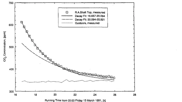
agreement behavior for different curve-fit periods on Thursday night is apparent from the Table 2 entries. The extreme of this behavior is indicated by the entries for the Friday-to-Saturday decay period (March 15-16, 1991) and is illustrated in Figure l2b, where again the curves fitted over totally distinct (i.e., no overlap} time periods are plotted for the same total time span. In this case, the earlier-fitted curve describes the overall concentration decay much better than· the later-fitted curve.
ASH RAE Transactions: Symposia
The
?-
and standard error estimates also suggest that thebest exponential curve fits are obtained during the earliest parts of the decay. This is somewhat surprising since the no-source assumption is violated more strongly earlier in the evening by more people being present in the building than later in the evening and in the early hours of the morning, when fewer people remain (ultimately only two security personnel overnight). (Because the concentrations in the late
evening and early hours of the morning are low, variations
in the outdoor concentration may have a greater effect than the few occupants remaining in the building.) The second curve-fit performed on the later half of Friday evening supports this conclusion, with poorer values for
?-
and the standard error estimate and a larger relative error in the air change rate. The early-morning curve-fit for the Wednesday-to-Thursday period, of necessity only for post-midnight data,1261
セセMMMMMMMMMMMMMMMMMMMMMMMMMMMMMMMMMMMM
...
0 R.A.Shaft Top, measured
Decay Fit: 16.657-20.094 Decay Fit: 20.094·25.921 600 Outdoors, measured 'E Jl; c'
セ@
E 500"
"
g
",,
"
'-o' ..."
400.--··
.... ···-····---· jッッlMMMセMMlMMMセセMMセMMセMMMMMMセMMMMMMセMMセMM⦅ェ@ 16 18 20 22 24 26 28Running Time lrom 00:00 Friday 15 March 1991, [h]
Figure 12b Comparison of fitted curves to C02 concentration data measured at the tops of the return air shafts during the end-of-day decay, March 15-16, 1991.
showed the extremes of deterioration in the
?
and standarderror estimate values, despite a relative error in the air
change rate that was only slightly worse than that obtained for analyses on early-evening data for the other days. The
major conclusion is that the air change rate is オョ、・イ・ウエゥュ。エセ@
ed by approximately 20% to 30% or more by using occu-pant-generated C02 as an active tracer gas for the simple decay technique at the end of a working day.
CONCLUSIONS
As a preface to the conclusions, it must be noted that several of the conclusions drawn from this study may apply only to the building tested. Such conclusions may not be applicable to other office buildings or other building types without first verifying them with some detailed measure-ments of air change rates and C02 concentrations in the particular building of interest.
The main conclusions from this study are the following.
1. This large but relatively uncomplicated office building
enjoys very good mixing. Also, the speed of mixing does not seem to depend on the relative percentages of recirculated and outdoor air in the supply air. For the purposes of tracer gas measurements of its air change rate, mixing times of 60 minutes were found to be sufficient.
2. Carbon dioxide concentration measurements at the tops of エィセ@ two main return air shafts are good representa-tions of the whole-building average concentrarepresenta-tions. This monitoring location would therefore be appropriate for
1262
the C02 sensor of a demand controller for the whole building. A correction factor of only a 2% to 4% increase would be needed for concentrations measured there to accurately represent average concentrations throughout the occupied zones of the building. 3. The daily peak and average carbon dioxide concentra·
tions are correlated well with the inverse of the air change rate, as predicted by Shaw's (1988) relationship. This may suggest a relatively universal applicability for that relationship, with minor correction factors for individual buildings of different types.
4. The outdoor air dampers and their controls in this building seem to be well calibrated in that their set percentage of outdoor air does result in an air change rate equal to the percentage of the air change rate that is delivered when set at 100% OA. The minimum outdoor air damper setting in this building is normally 20%, which provides 0.58 ach on average and a daily average carbon dioxide concentration of approximately 650 ppm.
5. Occupant-generated carbon dioxide proved to be a poor active tracer gas when simple decay analysis techniques were applied to the concentration decay at the end of the working day. The calculated air change rates were.
at best, approximately 20% to 30% less than the
air
change rates measured with sulfur hexafluoride tracer gas. Despite ignoring nonzero sources, the best results were obtained when the residual sources were largest, early in the decay period. The worst results were obtained when the fewest occupants remained in the building, later in the decay period.
REFERENCES
ASHRAE. 1989. ANSUASHRAE Standard 62-1989,
Ventila-tion for acceptable indoor air quality. Atlanta:
Ameri-can Society of Heating, Refrigerating and Air-Condi-tioning Engineers, Inc.
Persily, A.K., and W.S. Dols. 1989. The relationship of C02 concentration to office building ventilation. Air Change
Rate and Airtightness in Buildings, ASTM STP 1067,
M.H. Sherman, ed., pp. 77-92. Philadelphia: American Society for Testing and Materials.
Shaw, C.Y. 1988. Indoor air quality assessment in non-industrial buildings. Proceedings of the Fifth Canadian
Building and Construction Congress, Montreal,
No-vember 27-29.
Shaw, C.Y., R.J. Magee, C.J. Shirtliffe, and H. Unligil. 1991. Indoor air quality assessment in an office-library
building: Part I-T est methods. ASH RAE Transactions
97(2): 129-135.
DISCUSSION
1\Iark Lentz, Senior Project Engineer, PSJ Engineering, Inc., Milwaukee, WI: Was the outdoor air C02 concentra-tion always measured? What was the mechanism for outdoor
introduction? \Vas a continuous minimum source used, such as an injection fan, or was an outdoor air economizer used?
James T. Reardon: Yes, the concentration of C02 in the outdoor air was measured continuously in all tests. Outdoor air was introduced into the building via the outdoor air intake grille (with damper) and the supply air fan of each of
ASH RAE Transactions: Symposia
Smith, P.N. 1988. Determination of ventilation rates in occupied buildings from metabolic C02 concentrations and production rates. Building and Environment 23(2): 95-102.
Turiel, I., and J.V. Rudy. 1982. Occupant-generated C02 as
an indicator of ventilation rate. ASHRAE Transactions 88(1): 197-210.
Turner, W.A., D.W. Bearg, and J.D. Spengler. 1985. Building assessment techniques for indoor air quality evaluations. Environmental Engineering, Proceedings of the Specialty Conference, Boston. New York: American Society of Civil Engineers.
Vaculik, F. 1987. Air quality control in office buildings by a C02 method. IAQ '87: Practical Control of Indoor
Air Problems. Atlanta: American Society of Heating,
Refrigerating and Air-Conditioning Engineers, Inc. Woods, J.E., G. Winakor, E.A.B. Maldonado, and S. Kipp.
1982. Subjective and objective evaluation of a C02-controlled variable ventilation system. ASHRAE
Trans-actions 88(1 ): 1385-1408.
the (seven) HV AC systems in the building. No C02 was artificially introduced into the building. The only sources of C02 were the occupants themselves and the outdoor air supply to the building. For each test, the normally automatic controls for the HV AC systems were overridden and the dampers were set to provide a constant percentage of outdoor air for the complete test duration. All the HV AC systems were the constant-volume type. No economizer feature was active during any of the tests. As reported in this paper, the minimum percentage of outdoor air for any test (and for normal building operation) was 20%.