HAL Id: hal-03104965
https://hal.archives-ouvertes.fr/hal-03104965
Preprint submitted on 10 Jan 2021HAL is a multi-disciplinary open access
archive for the deposit and dissemination of sci-entific research documents, whether they are pub-lished or not. The documents may come from teaching and research institutions in France or abroad, or from public or private research centers.
L’archive ouverte pluridisciplinaire HAL, est destinée au dépôt et à la diffusion de documents scientifiques de niveau recherche, publiés ou non, émanant des établissements d’enseignement et de recherche français ou étrangers, des laboratoires publics ou privés.
Extremile Regression
Abdelaati Daouia, Irène Gijbels, Gilles Stupfler
To cite this version:
Extremile Regression
Abdelaati Daouia, Ir`ene Gijbels and Gilles Stupfler
∗†Toulouse School of Economics, France KU Leuven, Belgium
ENSAI & CREST, France
Abstract
Regression extremiles define a least squares analogue of regression quantiles. They are determined by weighted expectations rather than tail probabilities. Of special interest is their intuitive meaning in terms of expected minima and maxima. Their use appears naturally in risk management where, in contrast to quantiles, they fulfill the coherency axiom and take the severity of tail losses into account. In addition, they are comonotonically additive and belong to both the families of spec-tral risk measures and concave distortion risk measures. This paper provides the first detailed study exploring implications of the extremile terminology in a general setting of presence of covariates. We rely on local linear (least squares) check func-tion minimizafunc-tion for estimating condifunc-tional extremiles and deriving the asymptotic normality of their estimators. We also extend extremile regression far into the tails of heavy-tailed distributions. Extrapolated estimators are constructed and their asymptotic theory is developed. Some applications to real data are provided.
Keywords: Asymmetric least squares; Extremes; Heavy tails; Regression extremiles; Regression quantiles; Tail index.
∗Corresponding author.
†Abdelaati Daouia is Maˆıtre de Conf´erences, Universit´e Toulouse 1 Capitole, TSE, 21 all´ee de Brienne,
Manufacture des Tabacs, 31000 Toulouse, France (E-mail: abdelaati.daouia@tse-fr.eu). Ir`ene Gijbels is Professor of Statistics, KU Leuven, Statistics and Risk Section, Celestijnenlaan, 200b - box 2400, 3001 Leuven, Belgium (E-mail: Irene.Gijbels@kuleuven.be). Gilles Stupfler is Lecturer in Statistics, ENSAI & CREST, Campus de Ker Lann, 51 Rue Blaise Pascal, 35172 Bruz Cedex, France (E-mail:
1
Introduction
A basic tool in different scientific fields for analyzing the impact of a set of regressors X on the distribution of a response Y is quantile regression. For τ P p0, 1q, the conditional τ th quantile of Y given X “ x is defined as the minimizer
qτpxq P arg min
θPR E t r|τ ´ 1IpY ď θq| ¨ |Y ´ θ| ´ |τ ´ 1IpY ď 0q| ¨ |Y |s | X “ xu ,
(1) with 1Ip¨q being the indicator function. Subtracting |τ ´ 1IpY ď 0q| ¨ |Y | in the expectation makes the integrand well-defined and finite without assuming Ep|Y ||X “ xq ă 8. A disadvantage of quantile regression is that quantiles only use the information on whether an observation is below or above some specific value. However, in a financial risk manage-ment context for example, not taking into account the effective magnitude of high values of losses, might not be wise. Conditional expectiles deal with this drawback, and lead to coherent and more realistic risk measures as compared to quantile-based risk measures, as evidenced by [1] and [4], among others. The conditional τ th expectile is defined as
eτpxq “ arg min
θPR E
“
|τ ´ 1IpY ď θq| ¨ |Y ´ θ|2´ |τ ´ 1IpY ď 0q| ¨ |Y |2‰ | X “ x( , (2) obtained in a similar way to qτpxq in (1) but replacing absolute deviations by squared
deviations (Newey and Powell [8]). Expectiles depend on both the tail realizations and their probability, while quantiles only depend on the frequency of tail observations. An inconvenience of expectiles is their lack of transparent interpretation, due to the absence of a closed form expression of eτpxq as a solution to the asymmetric least squares problem (2),
for all τ ‰ 12. The absence of an explicit expression makes the treatment of expectiles a hard mathematical problem from the perspective of extreme value theory, for instance when it comes to estimating tail risk (Daouia et al. [4]).
Very recently, Daouia et al. [3] considered an alternative class to expectiles, called extremiles, which defines a new least squares analogue of quantiles. A starting point for the introduction of this class was that the unconditional τ th quantile of Y , with continuous cumulative distribution function F , can alternatively be obtained from
qτ P arg min
θPR E tJ
where Jτp¨q “ Kτ1p¨q, with Kτptq “ $ & % 1 ´ p1 ´ tqspτ q if 0 ă τ ď 1{2 trpτ q if 1{2 ď τ ă 1 (4)
being a distribution function with support r0, 1s, and rpτ q “ sp1 ´ τ q “ logp1{2q{ logpτ q. See Section 2.1 in [3]. The unconditional extremile of order τ is then defined by substi-tuting the absolute deviations with squared deviations, i.e.
ξτ “ arg min
θPR E
JτpF pY qq ¨
“
|Y ´ θ|2´ |Y |2‰( . (5) Unlike expectiles, extremiles can be motivated via several angles and enjoy various inter-pretations and closed form expressions. For an overview on this issue, and the specific merits related to these interpretations and explicit expressions, see Daouia et al. [3]. In the presence of covariates, one can define conditional extremiles by considering a condi-tional version of (5). It will be evidenced in Section2that conditional extremiles enjoy the same advantages as unconditional extremiles. Obviously statistical inference for condi-tional quantities, such as condicondi-tional quantiles, expectiles and extremiles, requires specific regression tools as compared to statistical inference for their unconditional counterparts. The aim of this paper is to study conditional extremiles, i.e. to pursue extremile regression, in a general setting. The main contributions of this paper consist of (i) dis-cussing probabilistic properties of regression extremiles; (ii) studying and establishing the asymptotic behaviour of their nonparametric estimators; (iii) investigating conditional extremile estimators when applied to the far tail (case τ “ τn Ñ 1, as the sample size
n Ñ 8); and (iv) illustrating the practical use of noncentral conditional extremiles. We shall discuss below in Section5 the various merits of extremile regression.
The paper is organized as follows. Section2presents the class of regression extremiles and their basic probabilistic properties. Section3deals with estimation of ordinary condi-tional extremiles for fixed orders τ . Extrapolated estimators of tail regression extremiles, for high orders τ “ τn Ñ 1 as n Ñ 8, are developed in Section 4 for heavy-tailed
condi-tional distributions. Section5concludes. All the necessary mathematical proofs, practical implementation guidelines and simulation results are given in the supplementary file.
2
Class of regression extremiles
Let X P Rd and Y P R be two random variables. Denote by F p¨|xq the cumulative
distribution function of Y given X “ x and by qτpxq “ F´1pτ |xq “ infty P R|F py|xq ě τ u
the related conditional quantile of order τ P p0, 1q. For ease of presentation, we assume throughout the paper that F p¨|xq is continuous. The order-τ extremile of this distribution function, as introduced in (5), defines the regression τ th extremile of Y given X “ x. Definition 1 Let Y given X “ x have a finite absolute first moment. Then, for any τ P p0, 1q, the conditional order-τ extremile of Y given X “ x is
ξτpxq “ arg min
θPR E
JτpF pY |Xqq ¨ r|Y ´ θ|2´ |Y |2s|X “ x( . (6)
Particularly useful is to look at ξτpxq as the following probability-weighted moment,
expected maximum or expected minimum.
Proposition 1 Let Y given X “ x have a finite absolute first moment. Then, for any τ P p0, 1q, we have the following equivalent closed form expressions:
ξτpxq “ E rY JτpF pY |Xqq |X “ xs “ ż1 0 Jτptq qtpxq dt “ ż1 0 qtpxq dKτptq, and ξτpxq “ $ & %
E rmax pYx1, . . . , Yxrqs when τ “ p1{2q1{r with r P Nzt0u,
E rmin pYx1, . . . , Yxsqs when τ “ 1 ´ p1{2q1{s with s P Nzt0u,
for independent observations Yxidrawn from the conditional distribution of Y given X “ x. In the central case τ “ 1{2, we have rpτ q “ spτ q “ 1, and hence ξτpxq reduces to the
standard regression mean EpY |X “ xq. The limit cases τ Ò 1 (i.e. rpτ q Ñ 8) and τ Ó 0 (i.e. spτ q Ñ 8) lead to the upper and, respectively, lower endpoints of the support of F p¨|xq. Further important properties are established in the following.
Proposition 2 (i) If Y given X “ x has a symmetric distribution with finite absolute first moment, then ξ1´τpxq “ 2 EpY |X “ xq ´ ξτpxq, for any τ P p0, 1q.
(ii) If Y “ mpXq ` σpXqε, where σpXq ą 0 and ε is independent of X and has a finite absolute first moment, then ξτpxq “ mpxq ` σpxqξτ,ε, for any τ P p0, 1q, where ξτ,ε denotes
An implication of Proposition 2 is that, for symmetric conditional distributions, the lower and upper extremile curves are symmetric about the regression mean. Also, the ex-tremile curves are parallel to each other if the distribution of the response is homogeneous. These properties hold for conditional quantiles as well.
3
Estimation method
Our approach is a local linear estimation based on the definition (6) which is of particu-lar relevance when considering flexible regression specifications such as local polynomial approximations. We restrict our analysis here to one-dimensional covariates X (d “ 1).
3.1
Least squares kernel smoothing
For a generic estimator pF p¨|xq of F p¨|xq, the local linear check function minimization solves the weighted least squares problem
arg min pα,βqPR2 n ÿ i“1 Jτ ´ p F pYi|xq ¯ tYi´ α ´ βpx ´ Xiqu 2 Lˆ x ´ Xi hn ˙ (7) to get the estimatorsα “ qq ξLL,τpxq and qβ “ qξ
1
LL,τpxq of ξτpxq and ξτ1pxq, respectively, where
Lp¨q is a kernel function and hn ą 0 a bandwidth sequence. Standard weighted least
squares theory leads to the following explicit solution ¨ ˝ q α q β ˛ ‚“ ´ XTLLWF ,Lp XLL ¯´1 XTLLWF ,Lp Y,
where Y is the column vector of dimension n containing all Yi, i “ 1, . . . , n, and XLL is
the usual design matrix of the local linear fitting technique, i.e. the n ˆ 2 matrix with a vector of 1’s as a first column, and where the second column consists of the values x ´ Xi,
i “ 1, . . . , n. Furthermore, the weight matrix in the weighted least squares problem is WF ,Lp “ diag ˆ Jτ ´ p F pYi|xq ¯ Lˆ x ´ Xi hn ˙˙ i“1,...,n .
Clearly, the asymptotic behavior of pF p¨|xq will be crucial to the analysis of the asymptotic and finite-sample behavior of qξLL,τpxq. Let us first discuss the properties of the latter
(C1) The random vector pX, Y q has a joint density fpX,Y q which is twice continuously
differentiable in its first argument and such that for each x0, we can write
sup
xPU
fpX,Y qpx, yq ` |BxfpX,Y qpx, yq| ` |Bxx2 fpX,Y qpx, yq|
(
ď hpyq
for some neighborhood U of x0, where h is a nonnegative measurable function
sat-isfyingş
Rp1 ` |y| 2`δ
qhpyq dy ă 8 for some δ ą 0;
(C2) The density fX of X is continuous and positive on the interior of its support;
(C3) The kernel L is a symmetric and bounded density function with compact support. Theorem 1 Assume that conditions (C1)–(C3) hold, and that pF p¨|xq is a uniformly con-sistent estimator of F p¨|xq satisfying
1 ? nhn n ÿ i“1 Jτ ´ p F pYi|xq ¯ tYi´ α ´ βpx ´ Xiqu ˆ x ´ Xi hn ˙j Lˆ x ´ Xi hn ˙ “ ?1 nhn n ÿ i“1 JτpF pYi|xqq tYi´ α ´ βpx ´ Xiqu ˆ x ´ Xi hn ˙j Lˆ x ´ Xi hn ˙ ` oPp1q (8)
locally uniformly in pα, βq P R2, for j “ 0, 1. Let hn Ñ 0 be such that nh5n Ñ 0, as
n Ñ 8. Then, for any x interior to the support of X, a nhn ! q ξLL,τpxq ´ ξτpxq ) d ÝÑ N ˆ 0, }L} 2 2 fXpxq Vτpxq ˙ , as n Ñ 8, (9) where Vτpxq “ E“Jτ2pF pY |xqq tY ´ ξτpxqu2 | X “ x‰.
Assumption (8) is evidently the central condition to be checked as part of Theo-rem 1. It ensures that the asymptotic analysis of qξLL,τpxq can be performed by replacing
p
F p¨|xq with F p¨|xq. It should also be noted that in the higher-dimensional setting with d´dimensional covariates X, nonparametric estimators converge in general at the rate ?
nhd, for a given bandwidth sequence h “ h
n Ñ 0. The associated bias condition, which
makes it possible to find the optimal rate of convergence of the estimator, is typically nhd`4 Ñ c P p0, 8q. This is realized for h having order n´1{pd`4q, resulting in the optimal convergence rate n2{pd`4q. This gets slower as d grows, and is an example of the well-known
The next corollary gives a simpler result for estimators pF p¨|xq having the typical rate of convergence n2{5. Examples of such estimators include the traditional
Nadaraya-Watson estimator [7], the nearest-neighbor estimator [9] and the (improved) local linear estimator [5]. For those estimators pF p¨|xq, we derive the asymptotic normality of qξLL,τpxq
when estimating noncentral regression extremiles ξτpxq.
Corollary 1 Assume that conditions (C1)–(C3) hold. Let pF p¨|xq be an estimator of F p¨|xq satisfying n2{5supyPR
ˇ ˇ
ˇF py|xq ´ F py|xqp ˇ ˇ
ˇ “ OPp1q. Let finally hn Ñ 0 be such that
nh5
n Ñ 0, as n Ñ 8. Then, with the notation of Theorem 1, for any x interior to the
support of X and any τ P p0, 1 ´ 1{?2s Y r1{?2, 1q, we have the convergence (9).
The condition τ P p0, 1 ´ 1{?2s Y r1{?2, 1q should not be viewed as a restriction in practice. Indeed, by Proposition 1, regression extremiles in the right tail (τ ě 1{2) are most easily interpreted when the power rpτ q “ logp1{2q{ logpτ q in (4) is an integer, since then ξτpxq “ E ” max ´ Yx1, . . . , Yxrpτ q ¯ı
, for independent observations Yxi drawn from the conditional distribution of Y given X “ x. In this case, the condition τ P r1{?2, 1q is equivalent to rpτ q ě 2, and hence all expected maxima and corresponding extremiles are covered by this condition, except for the conditional expectation ξ1{2pxq “ EpY |X “ xq
whose estimation obviously does not require extremile regression. Likewise, regression extremiles in the left tail (τ ď 1{2) are interpreted as ξτpxq “ E
” min ´ Y1 x, . . . , Y rp1´τ q x ¯ı
when rp1 ´ τ q P Nzt0u. In this case, the condition τ P p0, 1 ´ 1{?2s is equivalent to rp1 ´ τ q ě 2, and so apart from ξ1{2pxq “ EpY |X “ xq, all expected minima and
corresponding extremiles are covered by this condition.
3.2
Empirical data examples
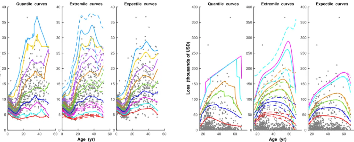
We now illustrate the usefulness of extremile regression on two real datasets about triceps skinfold variation and motorcycle insurance payouts. The first dataset ‘dataTriceps’, kindly sent by Keming Yu, comprises triceps skinfold measurements of 892 girls and women up to age 50, recorded in three Gambian villages during the dry season of 1989. To understand the evolution of triceps skinfold with age, Yu and Jones [12] proposed to
look at a collection of estimated quantiles as a function of age. The obtained fits via local linear check function minimization are graphed in Figure1(left panel). To calculate these conditional quantiles, we used the locally polynomial quantile regression function lprq of the R package quantreg, in conjunction with the optimal bandwidth hqτ chosen
by the Yu and Jones [12] selection method. The competing conditional extremiles qξLL,τ
in (7), obtained with the bandwidth hξτ from our automatic selection strategy developed
in Section B of the supplementary file, are given in the same figure (left panel) in solid lines, along with some 95% pointwise asymptotic confidence intervals in dashed lines. To calculate the probability weights Jτ
´ p F pYi|xq
¯
in qξLL,τpxq, we used in all our examples the
local linear estimator pF p¨|xq. In the absence of a rule-of-thumb bandwidth selection for estimated expectiles via the check function method of Yao and Tong [11], we superimpose in the same figure (left panel) the expectile curves corresponding to hqτ (dashed lines)
and those corresponding to hξτ (solid lines); the difference between the resulting expectile
curves is negligible although hqτ and hξτ are appreciably different for each τ .
The messages yielded by the three regression methods are broadly similar, indicating particularly that adulthood corresponds to a much greater variability in triceps skinfold compared to childhood. Still, expectiles beyond the regression mean exhibit less evidence of the obvious variation and over-dispersion of the triceps skinfold as age increases: the widening of extreme expectiles seems to be rather “narrow”. By contrast, there is a dis-tinct tendency for the noncentral extremiles and quantiles to be more spread, suggesting better capability of fitting both location and sparseness in data points. That said, extrem-ile regression seems to be beneficial at least in producing smoother and more pleasing fits of conditional location and spread beyond the regression mean. Of course, the quantile curves can be smoothed by resorting to local linear double-kernel smoothing, but this is unnecessary for extremiles. Moreover, we are not aware of any ready-made procedure for constructing asymptotic confidence intervals of conditional quantiles and expectiles based directly on the limit distributions of their local linear estimators.
The advantages of extremile regression at the tails become even more pronounced when considering heavy-tailed scenarios as is the case in most actuarial and financial
applica-tions. The second dataset ‘dataOhlsson’, available from the R package insuranceData, contains 670 motorcycle-related claims recorded from 1994 to 1998 by the Swedish in-surer Wasa. The scatterplot and local linear fits are given in Figure1(right panel). Here, tail regression extremiles show more alertness and reactivity to unexpected high losses than their expectile counterparts. They also exhibit better smoothness and stability than their quantile competitors and do not show any crossing, unlike the unpleasant quantile crossings that are incompatible with what occurs at the population level.
0 20 40 60 0 5 10 15 20 25 30 35 40 Triceps Skinfold Quantile curves 0 20 40 60 Age (yr) 0 5 10 15 20 25 30 35 40 Extremile curves 0 20 40 60 0 5 10 15 20 25 30 35 40 Expectile curves 20 40 60 0 50 100 150 200 250 300 350 400
Loss (thousands of USD)
Quantile curves 20 40 60 Age (yr) 0 50 100 150 200 250 300 350 400 Extremile curves 20 40 60 0 50 100 150 200 250 300 350 400 Expectile curves
Figure 1: Left panel: dataTriceps, with smoothed 1%, 3%, 10%, 25%, 50%, 75%, 90%, 97% and 99% quantile (left), extremile (middle) and expectile curves (right) in solid lines, and 95% pointwise asymptotic confidence intervals for ξ.01, ξ.1, ξ.5, ξ.9, ξ.99 in dashed lines.
Right panel: dataOhlsson, with smoothed 75%, 90%, 95%, 97%, 99% and 99.2% regression curves (solid), and confidence intervals for ξ.75, ξ.9, ξ.95, ξ.97 and ξ.99 (dashed).
Note that Proposition 1 provides a straightforward interpretation of the regression extremile ξτpxq by making use of the asymmetry level forms τ “ p1{2q1{rpτ q, for τ ě 1{2,
and τ “ 1 ´ p1{2q1{rp1´τ q for τ ď 1{2. Intuitively, for example in the case of
mo-torcycle insurance claims, in the right tail, ξτpxq ” ErmaxpYx1, . . . , Y rpτ q
x qs gives the
expected maximum claim amount among rpτ q potential claimants aged x years, with rp.97q « 22.75, rp.99q « 68.96, rp.992q « 86.29, rp.993q « 98.67, and rp.994q « 115.17. Interestingly, the regression quantile of the same order τ has the “dual” intuitive meaning as qτpxq ” MedianrmaxpYx1, . . . , Y
rpτ q
meaning of ξτpxq as an expected maximum on the right tail p12 ď τ ă 1q in the sense that E“max `Yx1, . . . , Y trpτ qu x ˘‰ ď ξτpxq ď E“max `Yx1, . . . , Y trpτ qu`1 x ˘‰ ,
where t¨u denotes the floor function.
4
Extremal regression
In this section, we focus on extremal regression of a response variable Y P R given a vector of covariates X P Rd. This translates into considering the order τ “ τ1
nÑ 1 or τn1 Ñ 0 as
the sample size n goes to infinity. To ease the presentation, we restrict our extreme-value analysis to the case τ Ñ 1. Similar considerations evidently apply to the left tail τ Ñ 0.
4.1
Model assumption
We assume for the sake of simplicity that the response Y given X “ x is positive and EpY |X “ xq ă 8. We focus on the challenging domain of attraction of heavy-tailed conditional distributions that better describe the tail structure and sparseness of the data in most applications in financial and natural sciences [2, 6, 10]. More precisely, we assume that the conditional tail quantile function t ÞÑ q1´t´1pxq is second-order regularly varying:
(E) @y ą 0, lim tÑ8 1 Apt|xq ˆ q1´ptyq´1pxq q1´t´1pxq ´ yγpxq ˙ “ yγpxqy ρpxq ´ 1 ρpxq
for some parameters 0 ă γpxq ă 1, ρpxq ď 0 and an auxiliary function Ap¨|xq having constant sign, with Apt|xq Ñ 0 as t Ñ 8. We use throughout the convention that pyb´ 1q{b “ log y for b “ 0, so that the right-hand side reads yγpxqlog y if the second-order parameter ρpxq is zero. The index γpxq ą 0 tunes the tail heaviness of the conditional distribution of Y given X “ x, with higher positive values indicating heavier conditional tails. The assumption γpxq ă 1 is tailored to our requirement that EpY |X “ xq ă 8.
4.2
Estimation procedure and main results
Here we consider the estimation of ξτpxq when τ “ τn1 Ò 1 at an arbitrary rate as n Ñ
distribution of Y given X “ x, that ξτ1
npxq „ qτn1pxq G pγpxqq as n Ñ 8, where Gpsq :“
Γp1 ´ sqtlog 2us and Γ is the Gamma function. This motivates the estimator
p ξ‹ τ1 npxq :“ pq ‹ τ1 npxq G ppγpxqq (10) obtained by substituting in suitable estimators qp‹
τ1
npxq of qτn1pxq and pγpxq of γpxq. Non-parametric local estimates of the tail quantities qτ1
npxq and γpxq have been proposed in
the last decade by [2, 6, 10], among others. Prominent among these contributions is the Weissman quantile-type estimator
p q‹ τ1 npxq ” pq ‹ τ1 n,τnpxq :“ ˆ 1 ´ τ1 n 1 ´ τn ˙´pγpxq p qτnpxq, (11)
where pγpxq andqpτnpxq are consistent estimators of γpxq and qτnpxq, with τnă τ 1
n being a
tuning sequence to be selected jointly with hn. Combining (10) and (11), we arrive at
p ξ‹ τ1 npxq ” pξ ‹ τ1 n,τnpxq “ ˆ 1 ´ τ1 n 1 ´ τn ˙´pγpxq p qτnpxq G ppγpxqq . (12) In Theorem A.1 in the Supplementary Material document, we establish the asymptotic distribution of pξ‹
τ1
npxq in its general form (12), for generic estimatorspγpxq andqpτnpxq, under
standard assumptions in the literature of conditional extremes. Here, we specialize the discussion to well-specified estimatorsqpτnpxq and pγpxq in the generic form (12) of pξ
‹ τ1
npxq.
We consider the Nadaraya-Watson type estimator pqτnpxq ” pF ´1 NWpτn|xq, where p FNWpy|xq :“ n ÿ i“1 1IpYi ď yqL ˆ x ´ Xi hn ˙O n ÿ i“1 Lˆ x ´ Xi hn ˙ . (13)
As for the choice of the conditional tail index estimator pγpxq, we will use in the sequel the notation αn :“ 1 ´ τn and pn:“ 1 ´ τn1, and consider the kernel estimator of [2]:
p γpxq “ J ÿ j“1 “logpq1´tjαnpxq ´ logqp1´αnpxq ‰ O J ÿ j“1 logp1{tjq, (14)
where p1 “ t1 ą t2 ą ¨ ¨ ¨ ą tJ ą 0q is a decreasing list of J weights. Note that, unlike [2],
we do not assume differentiability of the conditional distribution function, and therefore the distribution of Y given X is allowed to have atoms. The asymptotic normality of the corresponding regression extremile estimator
p ξ‹ 1´pnpxq :“ ˆ αn pn ˙γpxqp p q1´αnpxq G ppγpxqq
follows under the following additional regularity conditions:
(K1) The functions 1{γ and fX are Lipschitz continuous and x ÞÑ log `py|xq{ log y, where
`py|xq :“ y1{γpxq
r1 ´ F py|xqs, satisfies, for a norm } ¨ } on Rd, Dc ą 0, Dy0 ą 1, sup yěy0 ˇ ˇ ˇ ˇ log `py|xq log y ´ log `py|x1 q log y ˇ ˇ ˇ ˇ“ supyěy 0 1 log y ˇ ˇ ˇ ˇ log `py|xq `py|x1q ˇ ˇ ˇ ˇď c}x ´ x 1 }.
(K2) The kernel L is a bounded density with support included in the unit ball of Rd.
Theorem 2 Suppose (E) and (K1)–(K2) hold. Let x P Rd be such that f
Xpxq ą 0.
Assume further that ρpxq ă 0 and, as n Ñ 8, 1. αnÑ 0, nhdnαn Ñ 8 and nhdnpnÑ c ă 8; 2. logpαn{pnq{ a nhd nαn Ñ 0, nhd`2n αnlog2αn Ñ 0 and a nhd nαnApp1 ´ αnq´1|xq Ñ 0. Then we have a nhd nαn logpαn{pnq ˜ p ξ‹ 1´pnpxq ξ1´pnpxq ´ 1 ¸ d ÝÑ N ˆ 0, }L} 2 2 fXpxq VJγ2pxq ˙ as n Ñ 8, where VJ “ ˜ J ÿ j“1 2pJ ´ jq ` 1 tj ´ J2 ¸ O˜ J ÿ j“1 logp1{tjq ¸2 .
When choosing, for instance, the harmonic sequence tj “ 1{j, the variance of the
limiting distribution is minimal for J “ 9 with V9 « 1.25 (see [2]). We shall discuss below
concrete applications where ptj “ 1{jq1ďjď9 are employed with the discretized tuning
parameter αn “ k{n for a sequence of integers k P r1, nq. A data-driven method for
selecting both k and the bandwidth hn in practice is described in Supplement C.
4.3
Insurance payouts
This section returns to our motivating data set ‘dataOhlsson’ and explores estimation and inference for extreme risk associated with motorcycle insurance claims. It can be seen in Figure 1 that this data pn “ 670q features heavy tails and data sparsity in the tail areas. Figure 2 (top left) plots the tail index estimates pγpxq versus k, for the empirical
quartiles x of X. The plot shows stability over the region k P r50, 90s, which suggests to pick out the pointwise estimates pγpxq over this interval. The top right panel plots the final estimates pγpxq versus x obtained via our data-driven device (red curve), along with the estimates using k P t50, 70, 90u. It is remarkable that the automatic selection points towards similar results as these k values from the stable region. The four estimated curves indicate tail indicespγpxq P r0.25, 0.65s which, as expected, reflect a strong conditional tail heaviness. Hereafter in this extremal regression study, we focus mainly on the estimates obtained for x ď 55 to mitigate data scarcity and boundary effects beyond this range.
To estimate conditional extremiles ξτ1
npxq at extreme levels, Supplement D gives Monte
Carlo evidence that the extrapolated estimates pξ‹ τ1
npxq in (12) are more efficient relative
to the direct estimates qξLL,τ1
npxq from ordinary local linear regression in (7). For τ 1
n“ .99,
the middle panel of Figure2plots pξ‹ τ1
npxq versus k (left), for the empirical quartiles x of X,
and plots the final estimates x ÞÑ pξ‹ τ1
npxq (right), obtained by using the automatic selection
and three values of k (selected in the stable region r5, 25s of the plots shown on the left-hand side). The data-driven method affords a smoother and more stable estimated curve (in red). This extrapolated curve x ÞÑ pξ‹
τ1
npxq is superimposed in the bottom panel (left)
with the curve x ÞÑ qξLL,τ1
npxq of the local linear estimator (in solid blue), along with their
corresponding asymptotic pointwise 95% confidence intervals (in dashed blue for qξLL,τ1
npxq
and dashed red for pξ‹ τ1
npxq). There is a substantial difference between pξ ‹ τ1
npxq and qξLL,τn1pxq,
which may exceed 80,000 USD for claimants’ ages x outside the interval r30, 40s. The extrapolated quantile (Value at Risk) estimatorqp‹
τ1
npxq, described in (11), is also graphed
in the same figure (in dashed green). It lies below the extremile competitor (in solid red), close and sometimes beyond its lower confidence bound (in dashed red), with a gap that may exceed 54,000 USD. The extrapolated estimate pξ‹
τ1
npxq shows much greater reactivity
to the shape of the conditional tail, as can be observed on the right end of the plot where p
ξ‹ τ1
npxq visibly takes into account the few very large claims incurred by older customers to
produce a more prudent measure of extreme risk relative to these older claimants. The bottom right panel plots the extrapolated pξ‹
τ1
npxq and ordinary qξLL,τn1pxq
esti-mators of the tail extremile ξτ1
npxq ” ErmaxpY 1
x, . . . , Y rpτ1
nq
respectively, for τ1
n “ .992 [i.e. rpτn1q « 86], τn1 “ .995 [i.e. rpτn1q « 138] and τn1 “ .998
[i.e. rpτ1
nq « 346]. With the increase of the security level τn1, in contrast to the
non-extrapolated estimator qξLL,τ1
npxq, the refined version pξ ‹ τ1
npxq becomes clearly more alert to
the claims’ severity and better captures the magnitude of the two most extreme losses.
5
Concluding remarks
The use of regression extremiles appears naturally in the context of risk handling, where their interpretability is straightforward and they are fully operational in practice. Beyond their remarkable merits from the point of view of the axiomatic theory of risk measures, why should statisticians and practitioners care about extremile regression? A first dis-tinctive property of extremile regression is that, in contrast to its quantile and expectile competitors, the local linear estimators have an explicit form that is straightforward to compute, without recourse to any approximation algorithm. A second unexpected result is that the asymptotic variance of these estimators is not merely an adaptation to the conditional setup of the asymptotic variance arising in the unconditional case from [3]. In particular, this makes inference on regression extremiles much easier than inference on regression quantiles and expectiles. We are not aware of any ready-made procedure for constructing asymptotic confidence intervals of both conditional quantiles and expectiles based on the limit distributions of their local linear estimators. A further distinctive advantage of using local linear extremiles is that they suggest better capability of fitting both location and spread of data points beyond the regression mean, especially for heavy-tailed distributions. They provide much smoother and more stable fits than their quantile counterparts and do not suffer from crossings, as illustrated through both the concrete applications on triceps skinfold variation and motorcycle insurance payouts. In the class of light-tailed conditional distributions, population extremiles and quantiles are equiva-lent in the tail. In this class, the merits of local linear extremile estimators lead us then to favor their use over quantile estimators. It should finally be pointed out that we restrict our local linear kernel smoothing analysis to one-dimensional covariates. Extensions of our Theorem 1 and Corollary1 to multiple covariates are obviously of interest as well.
Acknowledgments
The authors are grateful to the Editor, an Associate Editor, and three reviewers for their very valuable comments, which led to a much improved presentation of the results. The re-search of A. Daouia and G. Stupfler is supported by the French National Rere-search Agency under the grant ANR-19-CE40-0013/ExtremReg project. A. Daouia also acknowledges funding from the ANR under grant ANR-17-EURE-0010 (Investissements d’Avenir pro-gram). I. Gijbels gratefully acknowledges support from the Research Fund KU Leuven (projects GOA/12/014 and C16/20/002), and from Research Grant FWO G0D6619N (Flemish Science Foundation). G. Stupfler also acknowledges support from an AXA Re-search Fund Award on “Mitigating risk in the wake of the COVID-19 pandemic”.
References
[1] Bellini, F., Klar, B., M¨uller, A. and Gianin, E.R. (2014). Generalized quantiles as risk measures. Insurance Math. Econom., 54, 41–48.
[2] Daouia, A., Gardes, L., Girard, S. and Lekina, A. (2011). Kernel estimators of ex-treme level curves. TEST, 20, 311–333.
[3] Daouia, A., Gijbels, I. and Stupfler, G. (2019). Extremiles: A new perspective on asymmetric least squares. J. Amer. Statist. Assoc., 114, 1366–1381.
[4] Daouia, A., Girard, S. and Stupfler, G. (2018). Estimation of tail risk based on extreme expectiles. J. R. Stat. Soc. Ser. B, 80, 263–292.
[5] Daouia, A. and Park, B.U. (2013). On Projection-Type Estimators of Multivariate Isotonic Functions. Scand. J. Stat., 40, 363–386.
[6] Goegebeur, Y., Guillou, A. and Osmann, M. (2017). A local moment type estimator for an extreme quantile in regression with random covariates. Comm. Statist. Theory Methods, 46, 319–343.
[7] Horv´ath, L. and Yandell, B.S. (1988). Asymptotics of conditional empirical processes. J. Multivariate Anal., 26, 184–206.
[8] Newey, W.K. and Powell, J.L. (1987). Asymmetric least squares estimation and test-ing. Econometrica, 55, 819–847.
[10] Stupfler, G. (2013). A moment estimator for the conditional extreme-value index. Electron. J. Stat., 7, 2298–2343.
[11] Yao, Q. and Tong, H. (1996). Asymmetric least squares regression and estimation: A nonparametric approach. J. Nonparametr. Stat., 6, 273–292.
[12] Yu, K. and Jones, M.C. (1998). Local linear quantile regression. J. Amer. Statist. Assoc., 93, 228–237.
0 50 100 150 200 250 300 0.0 0.2 0.4 0.6 0.8 1.0 1.2 Sample fraction k gamma(x) estimates
Tail index estimates vs k
25% quantile of x 50% quantile 75% quantile 0 50 100 150 200 250 300 0.0 0.2 0.4 0.6 0.8 1.0 1.2 20 30 40 50 0.2 0.3 0.4 0.5 0.6 0.7 0.8 Age x (yr) gamma(x) estimates
Tail index estimates vs x
optimal k k = 50 k = 70 k = 90 20 30 40 50 0.2 0.3 0.4 0.5 0.6 0.7 0.8 0 20 40 60 80 100 200 400 600 800 1000 Sample fraction k extremile(x) estimates
Tail extremile estimates vs k
25% quantile of x 50% quantile 75% quantile 0 20 40 60 80 100 200 400 600 800 1000 20 30 40 50 0 100 200 300 400 500 600 Age x (yr)
Estimates (thousands of USD)
o ooooooooooooooooooooooooooooo o o o o o o o o o o oo o o o o o o o oooooooo o o o o o o o o o o o o o o o o o o o o o o o o o o o o o o o o o o o o o o o o o o o o o o o o o o o o o o o o o ooooo o o o o o o o o o o o o o o o o o o o o o o o o o o o o o o o o o o o oo o o o o o o o o o o o o o o o o o o o o o o o o o o o o o o o o o o o o o o o o o o o o o o o o o o o o o o o o o o o o o o o o o o o o o o o o o o o o o o o o o o o o o o o o o o o o o o o o o o o o o o o o o o o o oooooooo o o o o o o o o o o o o o o o o o o o o o o o o o o o o o o o o o o o o o o o o o o o o o o o o o o o o o o o o o o o o o o o o o o ooo o o o o o o o o o o oooo o o o o o o o o ooo o o o o o o o o o oooooooo o ooo o o o o ooooooooooo o o o o o o o o o o o o oo o o o o o o o o o o o o o o o o o o o o o o o o o o o o oo o o o o o o o oo o o o o o o o o o o o o o o o o o o o o o o o o o o o o o o o o o ooo o o o o o o o ooooooo o o o o o o o o o o o o oo o o o o o o o o o o o o o o o o o o o o o o o o o ooooooooooo o o o o o o o o o oo o o o o o o o o o o oo o o o o o o o o ooooooooooo o o o o o o o o o o ooooooooooooooo o o o o o oooo o o ooo o o o o o
Tail extremile estimates vs x
optimal k k = 5 k = 15 k = 25 20 30 40 50 0 100 200 300 400 500 600 20 30 40 50 0 100 200 300 400 500 600 Age x (yr)
Estimates (thousands of USD)
o ooooooooooooooooooooooooooooo o o o o o o o o o o oo o o o o o o o oooooooo o o o o o o o o o o o o o o o o o o o o o o o o o o o o o o o o o o o o o o o o o o o o o o o o o o o o o o o o o ooooo o o o o o o o o o o o o o o o o o o o o o o o o o o o o o o o o o o o oo o o o o o o o o o o o o o o o o o o o o o o o o o o o o o o o o o o o o o o o o o o o o o o o o o o o o o o o o o o o o o o o o o o o o o o o o o o o o o o o o o o o o o o o o o o o o o o o o o o o o o o o o o o o o oooooooo o o o o o o o o o o o o o o o o o o o o o o o o o o o o o o o o o o o o o o o o o o o o o o o o o o o o o o o o o o o o o o o o o o ooooooooooooooooo o o o o o o o o ooo o o o o o o o o o oooooooo o ooo o o o o ooooooooooo o o o o o o o o o o o o oo o o o o o o o o o o o o o o o o o o o o o o o o o o o o oo o o o o o o o oo o o o o o o o o o o o o o o o o o o o o o o o o o o o o o o o o o ooo o o o o o o o ooooooo o o o o o o o o o o o o oo o o o o o o o o o o o o o ooooooooooooooooooooooo o o o o o o o o o oo o o o o o o o o o o oo o o o o o o o o ooooooooooo o o o o o o o o o o ooooooooooooooo o o o o o oooo o o ooo o o o o o Risk at tau = 0.99 EV extremile EV CI LL extremile LL CI EV quantile 20 30 40 50 0 100 200 300 400 500 600 20 30 40 50 0 100 200 300 400 500 600 Age x (yr)
Estimates (thousands of USD)
o ooooooooooooooooooooooooooooo o o o o o o o o o o oo o o o o o o o oooooooo o o o o o o o o o o o o o o o o o o o o o o o o o o o o o o o o o o o o o o o o o o o o o o o o o o o o o o o o o ooooo o o o o o o o o o o o o o o o o o o o o o o o o o o o o o o o o o o o oo o o o o o o o o o o o o o o o o o o o o o o o o o o o o o o o o o o o o o o o o o o o o o o o o o o o o o o o o o o o o o o o o o o o o o o o o o o o o o o o o o o o o o o o o o o o o o o o o o o o o o o o o o o o o oooooooo o o o o o o o o o o o o o o o o o o o o o o o o o o o o o o o o o o o o o o o o o o o o o o o o o o o o o o o o o o o o o o o o o o ooooooooooooooooo o o o o o o o o ooo o o o o o o o o o oooooooo o ooo o o o o ooooooooooo o o o o o o o o o o o o oo o o o o o o o o o o o o o o o o o o o o o o o o o o o o oo o o o o o o o oo o o o o o o o o o o o o o o o o o o o o o o o o o o o o o o o o o ooo o o o o o o o ooooooo o o o o o o o o o o o o oo o o o o o o o o o o o o o ooooooooooooooooooooooo o o o o o o o o o oo o o o o o o o o o o oo o o o o o o o o ooooooooooo o o o o o o o o o o ooooooooooooooo o o o o o oooo o o ooo o o o o o
Higher risks at tau = .992, .995, .998
EV extremile .998 LL extremile .998 EV extremile .995 LL extremile .995 EV extremile .992 LL extremile .992 20 30 40 50 0 100 200 300 400 500 600
Figure 2: Top left: plots ofpγpxq versus k, for the quartiles of X; Top right: estimates x ÞÑ p
γpxq obtained via the automatic selection (red) and three selected k values; Middle left: plots of pξ‹
.99pxq versus k; Middle right: final estimates x ÞÑ pξ.99‹ pxq; Bottom left: Estimates
p ξ‹
.99pxq and qξLL,.99pxq (solid red and blue), corresponding 95% confidence intervals (dashed
red and blue), andqp‹
.99pxq (dashed green); Bottom right: The estimators pξτ‹1
npxq (solid lines)
and qξLL,τ1
npxq (dashed lines), for τ 1