A portable and extensible performance model for stream-processing of XPath queries

(1)

HAL Id: hal-01195834

https://hal.archives-ouvertes.fr/hal-01195834

Submitted on 9 Sep 2015

HAL is a multi-disciplinary open access

archive for the deposit and dissemination of sci-entific research documents, whether they are pub-lished or not. The documents may come from teaching and research institutions in France or abroad, or from public or private research centers.

L’archive ouverte pluridisciplinaire HAL, est destinée au dépôt et à la diffusion de documents scientifiques de niveau recherche, publiés ou non, émanant des établissements d’enseignement et de recherche français ou étrangers, des laboratoires publics ou privés.

A portable and extensible performance model for

stream-processing of XPath queries

Muath Alrammal, Gaétan Hains, Mohamed Zergaoui

To cite this version:

Muath Alrammal, Gaétan Hains, Mohamed Zergaoui. A portable and extensible performance model for stream-processing of XPath queries. [Research Report] TR-LACL-2010-4, Université Paris-Est, LACL. 2010. �hal-01195834�

(2)

A portable and extensible performance model for

stream-processing of XPath queries.

Muath ALRAMMAL Ga´etan HAINS Mohamed ZERGAOUI

March 2010 TR–LACL–2010–4

Laboratoire d’Algorithmique, Complexit´e et Logique (LACL)

D´epartement d’Informatique

Université Paris 12 – Val de Marne, Faculté des Science et Technologie 61, Avenue du Général de Gaulle, 94010 Créteil cedex, France

(3)

Laboratory of Algorithmics, Complexity and Logic (LACL) University Paris 12 (Paris Est)

Technical Report TR–LACL–2010-4 M. ALRAMMAL, G. HAINS, M. ZERGAOUI

A portable and extensible performance model for stream-processing of XPath queries. c

(4)

Abstract

XML has become a standard for document storage and interchange and its convenient syntax improves the interoperability of many applications. The computational complexity and practical cost of XPath queries can vary dramatically so its unconstrained use leads to unpredictable space and time costs. Stream-processing of XPath queries mitigates this problem by restricting the query language fragment and allows simpler implementations by stack automata with no limit on the XML document size.

Wa have designed an accurate performance model for such algorithms. It collects static information about the XML document to statically predict the memory consumption of a query to within a few percent. The model is portable, adapts to any document structure and scales to 1GiB documents and beyond. In addition to predictable performance, user interac-tion with the system can lead to optimizainterac-tions by constraining the search for sub-documents.

Existing literature on this problem has not addressed all the technical problems involved and our model is to our knowledge the most complete of its kind.

1 Introduction

XML [25] has become a standard for document storage and interchange and its convenient syn-tax improves the interoperability of many applications. Yet the format is intrinsically costly in space and efficient access to XML data requires careful processing of XPath queries. Despite a logically clean structure, the computational complexity of XPath [5], XQuery[6] queries can

(5)

vary dramatically [24] [12]. As a result the unconstrained use of XPath leads to unpredictable space and time costs.

One proposed approach to combine the simplicity of XML data, the declarative nature of XPath queries and reasonable performance on large data sets is to impose their processing by purely streaming algorithms. The result is that queries must be restricted to a fragment of XPath but on the other hand processing space can be limited and very large documents can be accessed efficiently. But despite a relatively simple algorithm structure there are many parame-ters that influence processing space and time: the lazy vs eager strategy of the stack-automaton, the size and quantity of query results, the size and structure of the document etc. As a result the author of an XPath query may have no immediate idea of what to expect in memory consump-tion and delay before collecting all the resulting sub-documents. Given the very large variaconsump-tions in performance, this unpredictability can diminish the practical use of XPath stream-processing. To alleviate this situation we have designed an accurate performance model for stream-processing of XPath queries. Our model collects static information about the XML document and is then able to predict a priori the memory consumption of a query to within a few percent. This allows a user to either modify the query if predicted consumtion is too high, or to allow the algorithm to execute normally. We find that the model is completely portable: its prediction is also correct to within a small error on a different machine. Tests show that the error rate is stable from small documents to documents on the order of 1GiB and nothing prevents the model from being applied to much larger documents.

In a second application of our model we show how it can be used by the user to narrow the query’s search for sub-documents and thus put constraints on the streaming algorithm. With such an interaction between user and performance prediction, it is possible to improve sensibly the algorithm’s actual performance on a given query.

Predictable and efficient memory management is essential for practical stream processing so it was given top priority in our study. But we also have preliminary results for the prediction of processing time. Currently the model is able to predict time witin a factor of two for most queries. The processing time predictions also appear to be easily portable: a mostly constant factor relates predicted-measured time on one machine to the same values on a different machine. It should therefore be possible to project processing time from the model built on one machine to any other system quantified by a single benchmark.

In summary, we present a usable and reliable prototype for practical performance manage-ment of stream-processing for XPath queries on documanage-ments of any size and structure. Existing literature on this problem has not addressed all the technical problems involved and our model is to our knowledge the most complete of its kind.

The rest of this report is organized as follows: in section 2, we survey related work. Section 3 contains our motivations and objectives. In section 4, we present our performance model for stream-processing of XPath queries. Section 5 contains the experiments performed and their analysis. In section 6, we summarize our work and conclude in section 7 with also plans for future work.

2 Related work

Much research has been conducted to study the processing of XML documents in streaming fashion. The different approaches to evaluate XPath queries on XML data streams can be cat-egorized as follows (1) stream-filtering: determining whether there exists at least one match

(6)

of the query Q in the XML document D, yielding a boolean output. For example XTire [8]. (2) Stream-querying: finding which parts of D match the query Q. This implies outputting all answer nodes in a XML document D i.e. nodes that satisfy a query Q. An example of stream-querying research is XSQ [22].

Various stream-filtering systems have been proposed. XFilter [4], a filtering system, is the first one that addresses the processing of streaming XML data. In XFilter, each XPath query is transformed into a separate deterministic finite automaton (DFA). In YFilter [11], a set of XPath expressions is transformed into a single non-deterministic finite automaton (NFA) by sharing the prefix. Another filtering system is XTier [8] which supports tree shaped XPath expressions containing predicates. In XTier, a path expression is decomposed into several substrings each of which is a sequence of labels, then each substring is recorded in a table, called substring-table. The information in the table is used to check for partial matchings.

XPush machine [14] was proposed to improve the performance of stream-filtering. It pro-cesses large numbers of XPath expressions with many predicates per query on a stream of XML data. The XPush machine transforms each XPath expression into an NFA and by grouping the states in a set of NFAs, a single deterministic pushdown automaton (DPA) is constructed lazily. This is similar to the algorithm for converting an NFA to a DFA in the standard textbook on automata where stack automata are defined [16].

However, stream-filtering systems deliver whole XML documents which satisfy the filtering condition to the interested users. Thus, the burden of selecting the interesting parts from the delivered XML documents is left upon the users.

As a result, various stream-querying systems have been proposed. In TurboXPath [17] which is a lazy system for evaluating XQuery-like queries. The query input to TurboXPath is translated into a set of parse trees. Whenever a match of a parse tree is found within the data stream, the relevant data is stored in form of a tuple that is afterward evaluated to check whether predicate and join conditions are fulfilled. The output is constructed out of those tuples that have evaluated to true. Other systems are XSQ [22] and SPEX [21]. They propose a method for evaluating XPath queries over streaming data to handle closures, aggregation and multiple predicates. Their method is designed based on hierarchical arrangement of push-down transduc-ers augmented with bufftransduc-ers. An automata is extended by actions attached to states and a buffer to evaluate XPath queries. The main technique is a non-deterministic push-down transducer (PDT) that is generated for each location step in an XPath query. These PDTs are combined into a hierarchical pushdown transducer in the form of a binary tree. In [9] authors propose a lazy stream-querying algorithm TwigM, to avoid the exponential time and space complexity incurred by XSQ. TwigM extends the multi-stack framework of the TwigStack algorithm [7].

Gou and Chirkova [13] propose a lazy system for stream-querying called LQ. In this system the input query is translated into a table throughout stream processing and statically stored on the memory. Whenever a matching of XPath expression is found within the data stream, the evaluation process is applied only at the closing tag of the streaming element (root element of the XPath expression). LQ was proposed to handle two challenges of stream-querying that were not solved by [22] and [9]. These challenges are: recursion in the XML document and the existence of multiple copies the same label-node in the XPath expression. LQ is the algorithm used in our experiments and in section 4 we justify our choice of using this algorithm.

There has been some work to estimate the selectivity of path expressions for XML data. Most existing approaches solve the problem in a top-down manner, by capturing the full struc-ture of the XML data tree (or graph) with a synopsis strucstruc-ture and pruning it until a given

(7)

space constraint is satisfied.

These methods can be categorized by whether they are on-line or off-line, whether they han-dle twig queries or path queries only, whether they hanhan-dle leaf values.

Paper [10] proposed a correlated sub-path tree (CST), which is a pruned suffix tree (PST) with set hashing signatures that helps determine the correlation between branching paths when estimating the selectivity of twig queries. The CST method is off-line, handles twig queries, and supports substring queries on the leaf values. The CST is usually large in size and has been outperformed by [1] for simple path expressions.

In [1] authors propose two techniques for capturing the structure of XML data for estimating the selectivity of path expressions, these techniques are path trees and Markov tables.

The purpose of first technique is to construct a tree representing the structure of the XML data, which is called path tree. The constructed tree contains all the information required for selectivity estimation. The problem is the size of the path tree constructed form a large XML document, it is larger than the available memory for processing. Therefore, they summarize this tree to ensure that it fits in the available memory by deleting low-frequency nodes from anywhere in the tree. Then, they try to preserve some of the information represented in the deleted nodes at a coarser granularity by adding nodes (named *-nodes) to the path tree that represent groups of deleted nodes.

To estimate the selectivity of a path expression using a summarized path tree, they try to match the tags in the path expression with tags in the path tree to find all nodes in path tree to which the path expression leads. The estimated selectivity is the total frequency of all these nodes. When they cannot match a tag in the path expression to a path tree node with a regular tag, we try to match it to *-nodes

The Markov table approach starts with the full path-selectivity table of paths length up to a certain value. They construct a table of all the distinct paths in the data of length up to m and their frequency, where m is ≥ 2. The table provides selectivity estimates for all path expressions of length up to m. To estimate the selectivity of longer path expressions, They combine several paths using a specific formula.

The Markov Table (MT) method of [1] uses a fixed order Markov model to capture sub-path statistics in XML data. Queries on leaf values are not supported. The XPath- Learner method [20] extends the MT method [1] to an on-line method. In addition, XPathLearner supports exact match queries on leaf values using the Markov Histogram technique, which is a variant of Markov tables which additionally captures value distribution.

In [26] authors study the problem of dynamically estimating the selectivity for XML path expressions (on-line). They propose a compact estimator named Bloom Histogram (BH). It is a two-column table H(paths, v) where paths represents a set of paths in the XML document D and and v is a representative value for the frequency values of all path_i in paths. Given a path p, we can find from H a tuple Hi with p ∈ Hi.paths and return Hi.v as an estimation of the frequency of p in D.

In [27], authors propose a statistical learning approach called Comet (Cost Modeling Evo-lution by Training) for cost modeling of complex XML operators. This work is more oriented toward XML repositories consisting of a large corpus of relatively small XML documents. But as we will see in the experiments part, they also test their approach with large XML document. Their initial focus is on the CPU cost Model. To do that, they developed a CPU cost model

(8)

for XNAV operator which is an adaptation of TurboXPATH. Their idea was taking from pre-vious works in which statistical learning method are used to develop cost models of complex user-defined functions [15] and [18].

COMET is a hybrid of traditional relational cost modeling and a statistical learning ap-proach: some analytical modeling is still required, but each analytical modeling task is rela-tively straightforward, because the most complicated aspects of operator behavior are modeled statistically. The technique used to store the statistics is Path tree [1].

An advantage of COMET is that a XML query optimizer, through a process of query feed-back, can exploit COMET in order to be self-tuning. That is, the system can automatically adapt to changes over time in the query workload and in the system environment. The opti-mizer: estimates the cost of each operator in the query plan (navigation operator, join operator) and then combines their costs using an appropriate formula.

The statistical model can be updated either at a periodic intervals or when cost-estimation error exceed a specified threshold. Updating a statistical model involves either re computing the model from scratch using the current set of training data or using an incremental update method. In this approach they re-compute the model from scratch.

However, the synopsis constructed by using the techniques mentioned above (path trees, Markov tables, BH, CST) are still large in size. Even-though we use the compressed histogram approach [20], the size of synopsis is still large, particularly, if we want to process very large XML Data stream. In fact, if the model was to store all the tree’s paths or even all the tree’s sub-paths, it would require too much storage and would defeat the very purpose of streaming. To meet this requirement, in this paper we describe rules for accumulating compact performance information and propagating it to the given query to estimate the query cost.

3 Motivations and Objectives

As we mentioned before, data streaming is a necessary and useful technique to process very large XML documents but poses serious algorithmic problems. In addition, if the performance model needs to store all the paths or the sub-paths of the tree to estimate the query cost, it would require too much storage and would defeat the very purpose of streaming. Below we discuss a few of these challenges:

• Users/Applications constraints: An XML stream is the depth-first, left-to-right traversal of a (possibly unbounded) XML document [25]. Querying under memory constraints is unavoidable, because real applications do have real (hardware given) memory constraints. In order to avoid that the query evaluator crashes due to out-of-memory errors, memory constraints on the algorithm are necessary. Finally it enables query evaluation on small devices (mobile phone, PDA, etc.) with very limited memory.

• Developing cost models for query optimization is significantly harder for XML queries than for traditional relational queries. The reason is that XML query operators are much more complex than relational operators such as table scans and joins.

Path selectivity estimations is desirable in interactive and internet applications. The sys-tem could warn the end-user that his/her query is so coarse that the amount of results will be overwhelming, but it is not sufficient to model the query cost.

Knowing the answer’s interval of query X (the sub-fragment of the XML document which contains all answers of query X) is an another important parameter that should be con-sidered for modeling the query cost. For example: the existence of 5 answers for query X somewhere at the beginning of a very large XML document, might cost (Time/Memory)

(9)

less than finding one answer for query Y which is somewhere at the end of the same XML document.

This is why, we need to build a cost model for querying XML data stream which consider the path selectivity estimation and further important features.

• To our knowledge, COMET [27] is the first model proposed for addressing the query costing problem for XML data streams. The differences between our work and COMET are:

1. COMET is oriented toward XML repositories consisting of a large corpus of relatively small XML documents, while our purpose is to process both small and very large XML documents.

2. COMET considers the CPU time to model the query cost. The accuracy of the model for homogenous data-set is ranging between 3% and 17%. While in our model, we consider the memory allocated to model the cost for a given query and we present an attempt to estimate the CPU time for a given query.

3. The technique used to capture the structure of XML data and to store the statistics in OCMET is PathTree. According to [1] this technique is good for relatively small and heterogenous XML document. While in our model, we use a table of meta-data which contains several parameters used to predict the cost for a given query. Our technique functions well with the variant forms of XML documents (shape, depth, width).

• Importance of past queries: in streaming, sending a query to process very large XML data stream is a costly process, therefore learning from past queries is required to improve performance in a reasonable way. An example of past queries importance is that a 2005 study of Yahoo’s query logs revealed that 33% of the queries from the same user were repeated queries and that 87% of the time the user would click on the same result. This suggests that many users use repeat queries to revisit or re-find information [23].

Based on the above observations, we conclude that further optimizations for XML streaming are both required and possible. Our objectives are to build a portable and extensible perfor-mance model for stream-processing of XPath queries with the minimal storage possible. This model will later be used to improve the stream-querying process even though this improvement may decrease the possibility of finding all matches in the XML document.

Furthermore, we aim to build a user protocol which is an interactive mode used by the end-user to optimize the stream-querying querying process based on the end-user needs and resources. This protocol is the forth layer of our performance model, see figure 1.

In the next section, we introduce our proposal.

4 Performance Prediction Model

The performance model is a mathematical model of processing time and prediction. This model provides us in advance with the expected time/space to satisfy the XPath expression sent by the user. It consists of a large number of input (XPath,XML, Machine, meta-data) - response (measured time/space) pairs, used to construct an estimate of the input-performance relation-ship by capturing the underlying trends and extracting them from the noise. Then, a part of the information is discarded and the resulting model is used to predict the responses of the new input. More precisely, our performance model consists of:

(10)

PM-0.1:

XPath*SearchRange*XML*[Machine]− >predicted query evaluation cost (Time/Space)

LQ [13] was instrumented to provide us with the measured query evaluation cost for processing the concerned XPath. In PM-01, meta-data is the information needed to help us predict the query evaluation cost, it is explained in details in section 4.2. Furthermore, to optimize the stream-querying process, PM-01 augments implicitly the XPath with a part of the meta-data called search range to orient searching process. The impact of using the searching range on the performance (Time/Memory) is explained in details in section 5.3.1. In this syntax, we search over a subset of the XML document as specified by the search range (an interval in the sequence of input tokens). Notice that, the end-user will get a complete answer for his query.

If the resources predicted by PM-01 fit the end-user needs then, there is no need to use PM-0.2. Otherwise we use PM-0.2 which is described below.

PM-0.2:

XPath*ImposedValues*XML*[Machine]− >query evaluation cost (Time/Space)

To conduct further optimization on the stream-querying process we propose 0.2, it is PM-0.1 augmented with the value/s imposed by the end-user based on his needs and resources. For example: the end-user can impose the total amount of memory allocated by the program to process a query Q. Thus, PM-02 performs implicitly several mathematical estimations to adapt (recalculate the searching range) the stream-querying process with the value imposed by the end-users. PM-0.2 is explained in details in 4.4.

Figure 1: Layers of our Performance Model

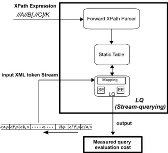
Below we explain in details each part of the performance prediction model (figure 1). 4.1 LQ (Lazy stream-querying)

To enable our experimental study we implemented the stream-query algorithm LQ of [13]. Our choice for this algorithm stems from the following raisons: (1) the authors in [13] explain the algorithm in detail, which is rare, thus facilitating the implementation process. (2) As we mentioned before, the query evaluation technique of LQ is lazy, thus easier to implement and instrument than an eager one. (3) Finally and most importantly, LQ was proposed to handle two challenges of stream-querying were not solved by [22] and [9]. These challenges are: recur-sion in the XML document and the existence of repetitions of the same label-node in the XPath expression. Based on that, the algorithm complexity (time/memory) of LQ is the best between the stream-querying systems mentioned in our related work. Our prototype OXPath was imple-mented using the functional language OCaml release 3.11 [19] which combines relatively high performance with strong typing and ML-language constructs for tree processing.

The current version of OXPath (figure 2) functions as follows:

OXPath takes two input parameters. The first one is the XPath expression that will be trans-formed to a query table statically using our Forward XPath Parser. After that, the main function

(11)

Figure 2: LQ (Lazy stream-querying)

is called. It reads the tree data-set line by line repeatedly, each time generating token. Based on that token a corresponding startBlock (SB) or endBlock (EB) function is called to process this token. Finally, the main function generates as output the query evaluation cost.

Query evaluation cost consists of:

• XPath: is any XPath with the following forms: //A, //A/B, //A/B/C, //A/B/C/D, //A[./B], where nodes A, B, C, D can be any node in the data-set. The semantics of query //A (respectively //A/B, //A/B/C, //A/B/C/D, //A[./B]) designates the sequence of all sub-documents rooted at a token labelled A (respectively rooted at a token labelled B son of a token labelled A, rooted at a token labelled C son of a token labelled B grandson of a token labelled A, ..., rooted at a token labelled A one of whose sons is labelled B). In the last form of query //A[./B], the [./B] condition is called a predicate. The number of nested sons in a query is called its number of steps.

• Steps: is the number of steps of the XPath Q.

• Cache: is the number of nodes (tokens) cached in the running-time stack during the processing of the query Q on the XML document D. These tokens correspond to the axis nodes of Q.

• Buffer: is the number of potential answer nodes (tokens) buffered during the processing of the query Q on the XML document D. These nodes correspond to the answer nodes of the query Q.

• NumberOfMatches: is the number of answer nodes (tokens) found during the processing of the query Q.

• Predicate: is the number of times we evaluate the predicate during the processing of the query Q on the XML document D.

• StartLT: the location of the tag of the first node X in the XML document order that corresponds to the root node of the XPath query Q.

• EndLT: the location of the tag of the last node Y in the XML document order that corresponds to the root node of the XPath query Q.

• MinTime: returns the processor time used by the program since the beginning of execu-tion till finding the first answer.

(12)

• AvgTime: (sum (time for each match))/total NumberOfMatches.

• MaxTime: returns the processor time used by the program since the beginning of exe-cution till the end of XML document processing.

• MinMemory: the total amount of memory allocated by the program since the beginning of execution till finding the first answer.

• AvgMemory: (sum (memory size for each match))/total NumberOfMatches.

• MaxMemory: the total amount of memory allocated by the program since the beginning of execution till the end of XML document processing.

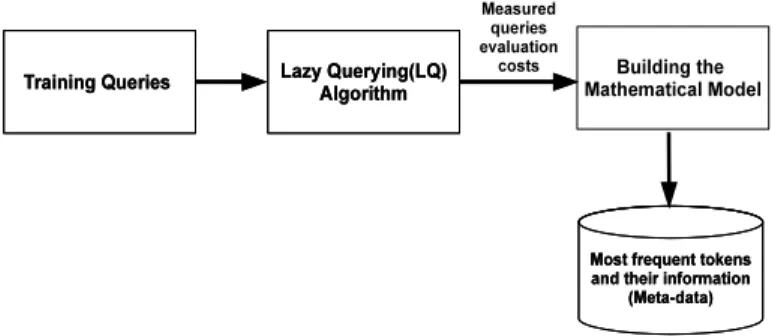
4.2 Building the Mathematical Model

As illustrated in figure 3, the first step is to send the training queries to collect the information needed (query evaluation cost) by using the stream-querying algorithm LQ. These information will be stored in a hash table. We call our technique for sending training queries and collecting the information exhaustive testing : a comprehensive process to test all possible not repeated XPaths existing in the data-set and having the following forms: //A/B, where A and B can be any element in the data-set.

The moment we have this information, we use them to build the mathematical model. Our mathematical model consists of s set of linear regressions for the following relations:

• MinTime vs (Buffer, Cache, StartLT, EndLT, Predicate). • AvgTime vs (Buffer, Cache, StartLT, EndLT, Predicate). • MaxTime vs (Buffer, Cache, StartLT, EndLT, Predicate). • MinMemory vs (Buffer, Cache, StartLT, EndLT, Predicate). • AvgMemory vs (Buffer, Cache, StartLT, EndLT, Predicate). • MaxMemory vs (Buffer, Cache, StartLT, EndLT, Predicate).

Figure 3: Building the Mathematical Model

To build the mathematical model predicting the value of MaxTime, we linearize the Max-Time vs (Buffer, Cache, StartLT, EndLT, Predicate) data points. The same process is applied on (MinTime, AvgTime, MinMemory, AvgMemory, MaxMemory) to obtain the overall query evaluation cost model.

To linearize MaxTime vs Buffer, we need first to calculate the slope and intercept of this relation by using the following functions:

val slope: (’a, float) Hashtbl.t -> (’b, float) Hashtbl.t -> float = <fun> val intercept: (’a, float) Hashtbl.t -> (’b, float) Hashtbl.t -> float = <fun> slopeMaxTimeVsBuffer:= (slope pathBuffer pathMaxTime) ;

(13)

Notice that, pathBuffer is the hash table which contains the values of Buffer for all queries which were launched during the exhaustive testing process. pathMaxTime is the hash table which contains the values of MaxTime for all queries which were launched during the exhaustive testing process. Based on this, the linear regression for the relation MaxTime vs Buffer is:

PredictedMaxTime = interceptMaxTimeVsBuffer +. slopeMaxTimeVsBuffer *. PredictedBuffer ;;

We calculate the linear regressions for the remaining relations of our mathematical model in the same way. In the next section 4.3, we explain how the prediction rules use these linear regressions to predict the query cost.

Once our mathematical model is built, all data in the hash table of the mathematical model will be discarded to free the memory. Then, we apply exhaustive testing, this time we use //A instead of //A/B. where A can be any element in the data-set. The advantage of the this process is to store frequent tokens and a part of their information (Cache, Buffer, NumberOfMatches, Predicate, StartLT, EndLT ) in a hash-table. These information is our meta-data which helps us to predict the query evaluation cost for the new-queries (End-user queries).

For a part of the real data-set TreeBank which consist of approximately 3000 tokens we found that the number of frequent tokens is 32, where frequent implies token A exists 3 times or more in the data-set.

4.3 Building the Prediction Model

In the previous section we described how to build the model and store the needed meta-data. We are then ready to receive the end-user queries. As illustrated in figure 4, the end-user sends his/her query to the analyzer: a function that analyses the query and estimates the values of the input parameters for the mathematical model by using the meta-data and applying the prediction rules.

val analyzer: int-> string-> string-> unit=<fun>

Each value of an input parameter will be used by its corresponding linear regression. To calculate the predicted MaxTime we use the following code:

let predictedMaxTimeValueBuffer = ((!slopeMaxTimeVsBuffer) *. (bSize) +. (!interceptMaxTimeVsBuffer)) in let predictedMaxTimeVsCache = ((!slopeMaxTimeVsCache) *. (cSize) +. (!interceptMaxTimeVsCache)) in let predictedMaxTimeVsStartLT = ((!slopeMaxTimeVsStartLT) *. (sLT) +. (!interceptMaxTimeVsStartLT)) in let predictedMaxTimeVsEndLT = ((!slopeMaxTimeVsEndLT) *. (eLT) +. (!interceptMaxTimeVsEndLT)) in print_string ("The predicted value of MaxTIme is ");

Printf.printf "\%.4f " ((absF(predictedMaxTimeValueBuffer +. predictedMaxTimeVsCache +. predictedMaxTimeVsStartLT +. predictedMaxTimeVsEndLT)/. 4.));

print_string ("s \n ");

Where, bSize is the value predicted of Buffer, cSize is the value predicted of Cache, sLT is the value predicted of StartLT, and eLT is the value predicted of EndLT.

In certain cases, we need to send partial queries (tokens) to enrich the meta-data if some parameter values are missing.

After that, the mathematical model will be fed with these parameters to output the pre-dicted query evaluation cost by using the appropriate formula.

Since collected data relates to individual tokens or small queries, and the input query is usually more complex, our model uses rules to propagate the cost information. Below we present those prediction or learning rules.

(14)

Figure 4: Building the Prediction Model

Token Cache Buffer Predicate-Evaluation matches StartLT EndLT

A 0 0 0 20 500 1500

B 0 0 0 15 700 2000

C 0 0 0 10 1000 2500

Table 1:Frequent tokens and their information (Meta-data)

4.3.1 Prediction Rules

Below, we demonstrate the learning rules of prediction through different cases. • Case (1): //A/B

Table 1 represents frequent tokens and their information. Note that these tokens are dis-tinct e.g. A <> B <> C. In this case, the prediction rules based are as follows:

– NumberOfMatches for token A will be an upper bound for the estimated value of Cache for XPath //A/B.

– NumberOfMatches for token B will be the upper bound estimated value of Buffer for XPath //A/B.

– NumberOfMatches for token B will be the upper bound estimated value of NumberOf-Matches for XPath //A/B.

– value of StartLT for token A will be the lower bound estimated value of StartLT for XPath //A/B.

– value of EndLT of token B will be the upper bound estimated value of EndLT for XPath //A/B. Table 2 shows the learning process from meta-data for this case.

By symmetry this case is also valid for the following XPath queries: //A/C, //B/A, //B/C, //C/A, //C/B.

• Case (2): //A/B/C

In this case, the prediction rules are:

– NumberOfMatches for token A plus those for B will be the upper bound estimated value of Cache for XPath //A/B/C.

– NumberOfMatches for token C will be the upper bound estimated value of Buffer for XPath //A/B/C.

– NumberOfMatches for token C will be the upper bound value of NumberOfMatches for XPath //A/B/C.

– The value of StartLT for token A will be the lower bound value of StartLT for XPath //A/B/C.

– The value of EndLT of token C will be the upper bound value of EndLT for XPath //A/B/C.

Table 3 shows the learning process from meta-data for this case. By symmetry this case is also valid for the following XPath: //A/C/B, //B/A/C, //B/C/A, //C/A/B, //C/B/A.

(15)

XPath Cache Buffer Predicate-Evaluation matches StartLT EndLT //A/B 20 15 0 0 500 2000

Table 2:End-user query and leaning from Meta-data

XPath Cache Buffer Predicate-Evaluation matches StartLT EndLT //A/B/C 35 10 0 10 500 2500

Existence of negative tokens among the frequent tokens:

A negative token is a token that does not belong to the XML data-set. In certain cases, this token can be a frequent one because it belongs to the most repeated queries sent by the end-users. Below, we demonstrate the possible learning rules of prediction through examples with re-spect to the following frequent tokens: A, B, C.

• Case (3): //A/B

Table 4 represents frequent tokens and their information. Note that token B is negative. In this case, the prediction rules are:

– NumberOfMatches for token A will be the upper bound estimated value of Cache for XPath //A/B.

– NumberOfMatches for token B will be the upper bound estimated value of Buffer for XPath //A/B, unless NumberOfMatches for token B is zero, in this case a message will be sent to the end-user informing him/her in advance that this query is negative.

This case is also valid for the following XPath: //C/B by symmetry. • Case (4): //B/A

NumberOfMatches for token B will be the upper bound estimated value of Cache nodes for XPath //A/B, unless NumberOfMatches for token B is zero, in this case, a message will be sent to the end-user informing him/her in advance that this query is negative. This case is also valid for the following XPath: //B/C by symmetry.

• Case (5): //A/B/C

Table 4 represents frequent tokens and their information. In this example, the prediction rules are:

NumberOfMatches for token A plus those for B will be the upper bound estimated value of Cache for XPath //A/B/C, unless NumberOfMatches for token B is zero, in this case, a message will be sent to the end-user informing him in advance that this query is negative. This case is also valid for the following XPath: //B/A/C by symmetry.

• Case (6): //A/C/B

Table 4 represents frequent tokens and their information. In this case, the prediction rules are:

– NumberOfMatches for token A plus those for C will be the upper bound estimated value of Cache for XPath //A/C/B.

– NumberOfMatches for token B will be the upper bound estimated value of NumberOf-Matches for XPath //A/C/B, unless NumberOfNumberOf-Matches for token B is zero, then a message will be sent to the end-user informing him in advance that this query is negative.

This case is also valid for the following XPath: //C/A/B by symmetry. Existence of predicates in the test queries:

(16)

A 0 0 0 20 500 1500

B 0 0 0 0 0 0

C 0 0 0 10 1000 2500

Table 4: Frequent tokens and their information (Meta-data)

A 0 0 0 20 500 1500

B 0 0 0 10 1000 2000

Test queries are the queries sent by the end-user. Below, we demonstrate the possible learning rules of prediction through examples with respect to the following frequent tokens: A, B (meta-data).

• Case (7): //A[./B]

– NumberOfMatches for token A will be the upper bound estimated value of Cache for XPath //A[./B] (because node A is the result node).

– NumberOfMatches for token B will be the upper bound estimated value of the number of times we evaluate the predicate B.

– The value of StartLT for token A will be the lower bound estimated value of StartLT for XPath //A[./B].

– The value of EndLT of token B will be the upper bound estimated value of EndLT for XPath //A[./B].

Table 6 shows the learning process from meta-data for this case. In this case, a stack will be created for the result node A because it is not a leaf node, therefore, each potential answer node A pushed in this sack will be considered as a Cache node.

This case is also valid for the following XPath: //B[./A] by symmetry. No information about a token (no meta-data):

As explained at the beginning of this document, it may not be practical to store information about unfrequent or less frequent tokens. Here we suggest possible solutions to this absence of information.

Below, we demonstrate the possible learning rules of prediction through examples with re-spect to the following frequent tokens: A, B, C (we do not have any information about the token C neither positive nor negative).

• Case (8): //A/B/C

– NumberOfMatches for token A plus those for B will be the upper bound estimated value of Cache for XPath //A/B/C. We obtain the meta-data of token C as follows:

We implicitly send the query //C to get its meta-data (In this case we obtained: Num-berOfMatches = 7 and EndLT = 1900), then:

• NumberOfMatches for token //C will be the upper bound estimated value of Buffer for XPath //A/B/C.

• StartLT for token A will be the lower bound estimated value of StartLT for XPath //A/B/C.

(17)

XPath Cache Buffer Predicate-Evaluation matches StartLT EndLT //A[./B] 20 0 10 0 500 2500

A 0 0 0 20 500 1500

B 0 0 0 15 700 2000

• EndLT for token C will be the upper bound estimated value of EndLT for XPath //A/B/C. Table 8 shows the learning process from meta-data for this case.

Sending implicitly the query //C is recommended because we send it only once to help us to predict the cost of the following XPath: //A/C/B, //B/A/C, //B/C/A, //C/A/B, //C/B/A, //A/C, //B/C, //C/A, //C/B and to know in advance whether the above mentioned queries are negative or not.

Repeated same-label node in the query sent:

The existence of repeated or same-label nodes in the query is a factor that increases the complexity of most stream-querying algorithms because we then need to buffer or cache a large number of nodes. Fortunately this problem is handled efficiently by LQ, see [13], but it still a challenge in our performance prediction model because our technique is based on storing information about frequent tokens to meet the purpose of the streaming process, which imply that our information is limited. Therefore, for the queries with same-label nodes the upper bound estimated values for buffer or cache is large.

Below, we demonstrate the possible learning rules of prediction through examples with respect to frequent tokens A, B (meta-data).

• Case (9): //A/A

– NumberOfMatches for token A minus 1 will be the upper bound estimated value of Buffer for XPath //A/A.

– NumberOfMatches for token A will be the upper bound estimated value of Cache for XPath //A/A.

This case is also valid for the following XPath: //B/B by symmetry. • Case (10): //A/A/B

– NumberOfMatches for token B will be the upper bound estimated vale of Buffer for XPath //A/A/B.

– NumberOfMatches for token A will be the upper bound estimated value of Cache for XPath //A/A/B.

This case is also valid for the following XPath: //B/B/A by symmetry. • Case (11): //A/B/A

– NumberOfMatches for token A minus 1, will be the upper bound estimated value of Buffer for XPath //A/B/A.

– NumberOfMatches for token A plus those for tken B will be the upper bound estimated value of Cache nodes for XPath //A/B/A.

(18)

XPath Cache Buffer Predicate-Evaluation matches StartLT EndLT //A/B/C 35 7 0 0 500 1900

XPath Cache Buffer Predicate-Evaluation matches StartLT EndLT

A 0 0 0 20 500 1500

B 0 0 0 15 700 2000

Table 9: End-user query and leaning from Meta-data

4.4 User Protocol

The user protocol is an interactive mode, it is used with our performance model to optimize the stream-querying process based on the end-user needs and resources. For example, the end-user can impose the total amount of memory allocated by the program to process a query Q. Thus, our model performs implicitly several mathematical estimations to adapt the stream-querying process with the value imposed by the end-users.

The interaction of the end-user with our model can be summarized as follows:

• Imposing the maximum time: he can impose the value of the processor’s time in seconds, used by the program to process a query Q. For example: the time imposed by the end-user to process query Q is 10s.

• Imposing the maximum memory: he can impose the value of the total amount of memory allocated by the program in KiB to process a query Q. For example: the memory imposed by the end-user to process query Q is 2048KiB.

• Imposing the maximum time and memory: he can impose the value of time and the value of memory allocated by the program to process a query Q. For example: the time imposed by the end-user to process query Q is 10s, and he memory imposed by the end-user to process query X is 2048KiB.

As mentioned above, the purpose of user protocol is to optimize the stream-querying process based on the needs and the resources of the end-user. In this case, we search over a subset of the XML document as specified by the search range (an interval in the sequence of input tokens). This process yields a stream-querying semi-algorithm which is an algorithm returning correct but possibly incomplete results. In other words sub-documents outside the search range are only scanned but not processed as an attempt to improve performance. This strategy is based on our earlier measurements [3] showing important gains when replacing stream-querying with stream-scanning.

To optimize the stream-querying process based on the resources (values of Time/Memory) imposed by the end-user, we need to determine the values of the searching range (StartLT, EndLT ).

Deciding the searching range (StartLT, EndLT )

As we mentioned before, our mathematical model consists of many linear regression functions, y = ax + b. The terms used in this section StartLT, EndLT, Buffer, Cache, MaxTime, and MaxMemory are already defined in section 4.1.

To determine the searching range (StartLT, EndLT ) based on the imposed value by the end-user, we present the following scenarios:

1. Time: the end-user imposes a limited time, e.g. maximum time is 15s. In this case, we calculate the values of StartLT and EndLT of the searching range as follows:

• EndLT : in our mathematical model, the value of the maximum time is the absolute average value obtained from the following relations:

(19)

ValueOfMaxTimeVsStartLT=((slopeMaxTimeVsStarLT)*.(StartLT)+.(interceptMaxTimeVsStartLT)) ValueOfMaxTimeVsEndLT=((slopeMaxTimeVsEndLT)*.(EndLT)+.(interceptMaxTimeVsEndLT)) ValueOfMaxTimeVsBuffer=((slopeMaxTimeVsBuffer)*.(Buffer) +.(interceptMaxTimeVsBuffer)) ValueOfMaxTimeVsCache=((slopeMaxTimeVsCache)*.(Cache)+.(interceptMaxTimeVsCache))

Therefore, the value of EndLT is the absolute average integer value obtained from the following relations:

StartLT=(ValueOfMaxTimeVsStartLT/. slopeMaxTimeVsStartLT)-.(interceptMaxTimeVsStartLT). EndLT=(ValueOfMaxTimeVsEndLT/. slopeMaxTimeVsEndLT)-.(interceptMaxTimeVsEndLT). Buffer=(ValueOfMaxTimeVsBuffer/. slopeMaxTimeVsBuffer)-.(interceptMaxTimeVsBuffer). Cache=(ValueOfMaxTimeVsCache/. slopeMaxTimeVsCache)-.(interceptMaxTimeVsCache).

• StartLT : to make sure that stream-querying process will start from the right position in the XML document, we get the value of StartLT from our meta-data based on the query sent by the end-user.

val getStartLT->string->float=<unit>

Once we have the values of searching range (StartLT, EbdLT), we augment them to the end-user’s query to optimize the stream-querying process.

2. Memory: end-user imposes a limited Memory, e.g. maximum memory is 15000KiB. In this case, we calculate the values of StartLT and EndLT of the searching range as follows:

• EndLT : in our mathematical model, the value of the maximum memory is the absolute average value obtained from the following relations:

ValueOfMaxMemoryVsStartLT=((slopeMaxMemoryVsStarLT)*.(StartLT)+.(interceptMaxMemoryVsStartLT)) ValueOfMaxMemoryVsEndLT=((slopeMaxMemoryVsEndLT)*.(EndLT)+.(interceptMaxMemoryVsEndLT)) ValueOfMaxMemoryVsBuffer=((slopeMaxMemoryVsBuffer)*.(Buffer)+.(interceptMaxMemoryVsBuffer)) ValueOfMaxMemoryVsCache=((slopeMaxMemoryVsCache)*.(Cache)+.(interceptMaxMemoryVsCache))

Therefore, the value of EndLT is the absolute average integer value obtained from the following relations:

StartLT= (ValueOfMaxMemoryVsStartLT/. slopeMaxMemoryVsStartLT)-.( interceptMaxMemoryVsStartLT). EndLT= (ValueOfMaxMemoryVsEndLT/. slopeMaxMemoryVsEndLT)-.( interceptMaxMemoryVsEndLT).

Buffer= (ValueOfMaxMemoryVsBuffer/. slopeMaxMemoryVsBuffer)-.( interceptMaxMemoryVsBuffer). Cache= (ValueOfMaxMemoryVsCache/. slopeMaxMemoryVsCache)-.( interceptMaxMemoryVsCache).

Once we have the values of searching range (StartLT, EbdLT), we add them as meta-data to the end-user’s query to optimize the stream-querying process.

3. Time Memory: the end-user imposes a limited time, e.g. maximum time is 15s, and he imposes a limited Memory e.g. maximum memory is 15000KiB. In this case, we calculate the values of StartLT and EndLT of the searching range as follows:

• EndLT : to find a solution for this case, we calculate the maximum time and the maximum memory in the same way that we explained above. Then, the new value of EndLT will the min value of EndLT (maximum time) and EndLT (maximum memory)

EndLT= min (EndLT(Maxumimum time)) ( EndLT(Maximum Memory))

(20)

Below, we present the interactive mode with the end-user. Interactive mode with the end-user

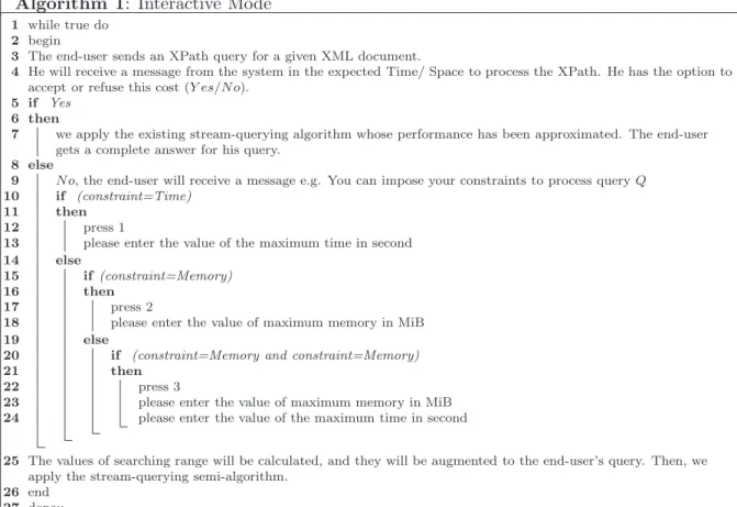
Once the mathematical model is built and the meta-data is stored, the end-user can interact with our model as it is explained in algorithm 1.

Algorithm 1: Interactive Mode while true do

1 begin 2

The end-user sends an XPath query for a given XML document. 3

He will receive a message from the system in the expected Time/ Space to process the XPath. He has the option to 4

accept or refuse this cost (Y es/N o). if Yes

5 then 6

we apply the existing stream-querying algorithm whose performance has been approximated. The end-user 7

gets a complete answer for his query. else

8

N o, the end-user will receive a message e.g. You can impose your constraints to process query Q 9 if (constraint=Time) 10 then 11 press 1 12

please enter the value of the maximum time in second 13 else 14 if_{(constraint=Memory)} 15 then 16 press 2 17

please enter the value of maximum memory in MiB 18

else 19

if (constraint=Memory and constraint=Memory) 20

then 21

press 3 22

please enter the value of maximum memory in MiB 23

please enter the value of the maximum time in second 24

The values of searching range will be calculated, and they will be augmented to the end-user’s query. Then, we 25

apply the stream-querying semi-algorithm. end

26 done;; 27

An example of using our user protocol is as follows:

1. The end-user inserts the name of data-set to construct the mathematical model and to store the meta-data, see figure 5.

Figure 5: Building the mathematical Model

2. Then, he is asked to insert the name of data-set and the query concerned to execute his search. He will receive a massage from the system in the expected Time/ Space to process the XPath. He has the option to accept/refuse this cost, see figure 6.

3. In our case, we suppose that the end-user did not accept this cost, therefore he chose the option N o to optimize his search, see figure 7.

(21)

Figure 6: Predicting the cost of the query sent

Figure 7: Refusing the predicted query cost

4. The end-user decided to optimize the time, therefore he pressed 1, then he imposed a new value for the maximum time, see figure 8.

Figure 8: Optimizing the query by imposing constraints

The value of maximum time imposed by the end-user is 0.004s. As we see in the figure above, the value of MaxTime was reduced from 0.009s to 0.004s. Also, NumberOfMatches reduced from 9 matches to 5 matches.

5 Experimental Results

In this section, we demonstrate the accuracy of our model by using variety of XML data-sets. In addition, we examine its efficiency and the size of the training set and meta-data that it requires. For example, the latter should not be too large in practice and we observe that our model behaves favorably in this respect. Meta-data build from frequent (repeated 3 times or more) tokens in the document occupies only 1/2000th of the document size, and this is confirmed for tests on documents differing in content, structure and size.

(22)

synthetic synthetic TreeBank TreeBank Structure wide wide narrow deep narrow deep

and shallow and shallow and recursive and recursive Data Size 43MiB 1GiB 64KiB 146MiB Max./Avg Depth 10/4.5 10/4.5 36/7.6 36/7.6

Table 10: Characteristics of the experimental data-sets.

5.1 Experimental Setup

We performed experiments on a MacBook with the following technical specifications: Intel Core 2 Duo, 2.4 GHz, 4 GiB RAM. Then, we checked the portability of the model to Red hat Linux with the following specifications: Intel Xeon 2.6 GHz, 8 GiB RAM.

We used synthetically generated data-sets and data-sets from a real-world application. See table 10. The Objective Caml language version 3.11 was used on both machines.

In the first part of our experiments, we measured the quality of the model prediction (section 5.2). While in the second part (section 5.3), we presented the impact of using meta-data in our model on the performance. In the end (section 5.4), we showed that our model is easily portable. 5.2 Quality of Model Prediction

To test the quality of the model prediction we performed several experiments for measuring space prediction. We measured the space prediction of the model without the interaction of the end-user, in this syntax, the end-user accepts the predicted query evaluation cost (predicted allocated memory) and does not impose any constraint. Then, the quality of space prediction was measured once the end-user imposes memory constraints to optimize his search.

Though the purpose of our model is to measure the space prediction, we also presented an attempt to measure the time prediction for a given query.

5.2.1 Space Prediction

1. No Interaction Between the End-user and the Model:

The quality of prediction (error percentage) of our model was measured for both real and synthetic data-sets. We first measured the quality of prediction by using the real data-set TreeBank which has a narrow and deep structure and a size of 64KiB. Figure 9 illustrates the percentage error of our prediction for the query evaluation cost. As can be seen, the error average for space is 3.80%.

Figure 9: Percentage error- TreeBank 64KiB

Our motivating scenario is to process large XML documents and considering the memory allocated to model the cost for a given query. Therefore, we measured the quality of prediction by using the real data-set TreeBank which has a narrow and deep structure and it has a size of 146MiB.

Figure 10 illustrates the error percentage of query evaluation cost. As can be seen, the error average of space is 9.87%.

(23)

Figure 10: Percentage error- TreeBank 146MiB

Furthermore, we measured the quality of prediction by using a synthetic data-set which is wide, shallow and it has a size of 1GiB (see table 10). Figure 11 illustrates the error percentage of query evaluation cost. As can be seen, the error average of space is 7.44%.

Figure 11: Percentage error- Synthetic 1GiB

2. Interaction Between the End-user and the Model:

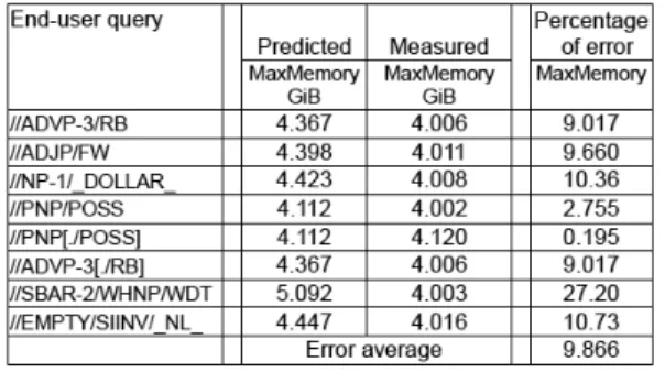
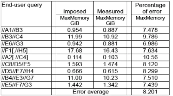
As we mentioned above, the end-user can impose certain constraints to optimize his queries by using the user protocol. We measured the quality of prediction of user protocol by using the data-set treeBank 146MiB. Figure 12 illustrates the percentage of error between the values imposed by the end-user and the measured ones by the model for certain queries. As can be seen, the error average for space is 18.48%.

Figure 12: Percentage error of user protocol - TreeBank 146MiB

We also measured the quality of prediction of the user protocol by using the synthetic data-set 1GiB. Figure 13 illustrates the percentage of error between the values imposed by the end-user and the measured ones by the model for certain queries.

(24)

Figure 13: Percentage error of user protocol - Synthetic 1GiB

5.2.2 Time Prediction

The quality of prediction (error percentage) of our model was measured by using real data-sets. We first measured the quality of prediction by using the real data-set TreeBank which has a narrow and deep structure and a size of 64KiB. Figure 14 illustrates the percentage error of our prediction for the query evaluation cost. As can be seen, the error average for time is 4.45%.

Figure 14: Percentage error for time- TreeBank 64KiB

We also measured the quality of prediction by using the real data-set TreeBank which has a narrow and deep structure and it has a size of 146MiB. Figure 15 illustrates the error percentage of query evaluation cost. As can be seen, the error average of time is 69.64%.

Figure 15: Percentage error for time- TreeBank 146MiB

5.3 Impact of Using Meta-data in our Model on the Performance. 5.3.1 Improving the Performance with Searching range (PM-0.1)

In the PM-0.1 we restrict search to a subset of the XML document as specified by a specific part of the meta-data. The definition of stream-querying implies outputting all matches in XML doc-ument D which satisfy query Q. This is challenging in situations such as using a portable devices with limited resources (small memory size) with very large XML documents, or having a hard time limit during which the user can wait for the answers. To alleviate this problem, we define

(25)

Figure 16: An XML document and its SAX parser events

stream-scanning: to process the XML data stream with minimal resources, this process simply searches the position of a specific element in D without caching nor buffering. Here caching is to cache specific nodes of the XML document D in run-time stacks, these nodes correspond to the axis node of the query Q, and buffering consists in buffering the potential answer nodes of D. The concept introduced by our PM-0.1 is to rely on the structure of the document, the in-formation it contains for estimating performance as before, and what we call Oriented XPath: an XPath query augmented with searching range for orienting the search as described below. The searching range is a meta-data augmenting the XPath expression with two points: StartLT and EndLT which were already defined in section 4.2. Together StartLT and EndLT define an interval within which streaming operates, with pure scanning elsewhere before StartLT.

To explain the idea of searching range, we present the example below:

Figure 16 represents an XML document and its events generated by the SAX parser. In figure 16 (B) the integer number to right of each event of the SAX parser represents the location of the tag of the corresponding event (element in the XML document). Based on this example, the values of StartLT and EndLT of the XPath //L/M are 4 and 8 respectively.

The idea is to first learn from frequent tokens in advance those parts of the document that contain the information to be found. This information may also be explicitly provided by the user of a querying interface, for example one may want to search a very large document knowing that the information sought is located in the second half of the document.

To show the efficiency of a restricted searching range compared to the existing exhaustive stream-querying algorithm LQ, we performed two type of tests on the data-set treeBank 146MiB, these tests are:

T1: queries were sent without searching range.

T1′_{: same queries were sent with searching range obtained from T1 to demonstrate the time/memory} gain possible.

Figure 17 shows the query evaluation costs (time) of T1 and T1′_{. MinTime of T1 is 2.07s} while for T1′ _{it is 1.75s. The 15% gain in time is due to stream scanning until reaching the} StartLT point, thus avoiding unnecessary buffering and caching processes. AvgTime of T1 is 5.57s while for T1′ _{is 5.22s, the slight gain of time occurred because the gain of time of MinTime} affects positively the value of AvgTime. MaxTime for T1 is 13.05s while for T1′ _{it is 8.46s. The} gain of 37% in time is due to both StartLT and EndLT restrincting the search range so that stream-querying stops the moment EndLT is reached. This is correct because we know that there will be no any further possible matches in the XML document.

(26)

Figure 17: Query evaluation cost for T1 and T1′

Figure 18: Query evaluation cost for T1 and T1′

is 635MiB while for T1′ _{it is 512MiB the gain of memory which is 20% was obtained because} of the stream scanning technique which scans the XML document until StartLT is reached. AvgMemory of T1 is 2035MiB while for T1′ _{it is 1703MiB, a gain of 17% in memory appears} because the gain on MinMemory affects positively the value of AvgMemory. MaxMemory value for T1 is 4115MiB while for T1′ _{it is 2584MiB. The gain of 38% in memory is due to the use} of both StartLT and EndLT to delimit the searching range. Thus we stop the stream-quering process the moment EndLT is reached because we know that there will be no any further possible matches in the document.

5.3.2 Negative queries

In this section, we present the impact of using meta-data on the measured Time/Memory for the negative queries. As we mentioned in 4.3.1 (prediction rules), frequent negative tokens help us to decide in advance that certain queries are negative. This property which exists in the model improves the performance.

To show the efficiency of our model compared to the existing exhaustive stream-querying algorithm LQ, we performed two type of tests on the data-set treeBank 146MiB, these tests are: T2: negative queries were sent without meta-data.

T2′_{: same queries were sent with meta-data obtained from T2 to demonstrate the time/memory} gain possible for negative queries.

Figure 19 shows the query evaluation costs (time) of T2 and T2′_{. The values of MaxTime} of T2 and T2′ _{for the first 5 queries are equal 69.5s, because the model still did not detect any} frequent negative token. The values of MaxTime of T2 for the first 10 queries is 134.12s while for T2′ _{is 122s, the time improvement of T2}′ _{occurred because the model detected in advance}

(27)

Figure 19: Impact of metadata on time for T2 and T2′

that one query is negative. The values of MaxTime of T2 for the first 15 queries is 207.5s while for T2′ _{is 160.2s, the time improvement of T2}′ _{occurred because the model detected in advance} that three queries are negative. The values of MaxTime of T2 for the all queries is 268.35s while for T2′ _{is 187s, the time improvement of T2}′ _{which is 30% occurred because the model detected} in advance that six queries are negative.

Figure 20: Impact of metadata on memory for T2 and T2′

Figure 20 shows the query evaluation costs (memory) of T2 and T2′_{. The values of} MaxMem-ory of T2 and T2′ _{for the first 5 queries are equal 20.11GiB, because the model still did not} detect any frequent negative token. The values of MaxMemory of T2 for the first 10 queries is 40.13GiB while for T2′ _{is 36.13GiB, the memory improvement of T2}′ _{occurred because the} model detected in advance that one query is negative. The values of MaxMemory of T2 for the first 15 queries is 60.31 GiB while for T2′ _{is 48.14GiB, the memory improvement of T2}′ _occurred because the model detected in advance that three queries are negative. The values of MaxMem-ory of T2 for the all queries is 80.42GiB while for T2′ _{is 56.21GiB, the memory improvement of} T2′ _{which is 30% occurred because the model detected in advance that six queries are negative.} 5.4 Model Portability on other Machines

To check the portability of our model, we rebuilt it on another machine running a version of Linux and with a different architecture. We used the same byte-code object file which we already used in the test of figure 9. Also, we used the same data-set treeBank of size 46KiB and the

(28)

same queries used in figure 9. Figure 21 illustrates the error percentage of query evaluation cost. As can be seen, the error average for space is 3.79%.

Figure 21: Percentage error- TreeBank 64KiB(Linux)

We conclude that:

- Memorylinux = Memorymac.

which is a stable factor for converting our model accross the two systems we used. It would thus appear that our model is easily portable.

6 Conclusion

In this paper we presented our performance prediction model for queries on XML documents in a fragment of XPath. The model allows static a priori prediction of time-space parameters on a given (variable) query for a given (fixed) XML data-set. It proceeds by accumulating information from past queries whose tokens are those frequently found in the target document. Two specific objectives for our model were:

1. to obtain reliable and portable cost predictions for random queries on a fixed data-set, while storing a small amount of meta-data.

2. to use the predictions to improve performance and/or resource management.

Our first objective was achieved by constructing the model with the minimal storage needed for the analyzer to predict query evaluation costs. The size of frequent queries and their infor-mation (meta-data) for the data-set TreeBank (deep and recursive, many repeated same-label nodes, 146MiB) is 42KiB. While for the synthetic data-set (wide and shallow, fewer repeated same-label nodes than treeBank, 43MiB) the size of meta-data is 24KiB.

The second objective is to improve the stream-querying process. This objective was fulfilled by using searching ranges to alternate between streaming and querying. As we showed in our experiment, the gain of MaxTime reached up to 38%, while the gain of MaxMemory reached 37%. Furthermore, meta-data improved the performance (Time/Memory) for negative queries, as we shown in our experiments the gain of MaxTime reached up to 30%, and the gain of MaxMemory reached 30%.

7 Future Work

We aim to extend and improve the performance model by considering a larger fragment of XPath to include all of the Forward XPath defined in [2].

Our current non optimized model building processes from 100 to 1000 token/s which is maybe slow for very large XML documents.

(29)

To ensure accurate XML path selectivity estimation, our mathematical model and meta-data must be updated once the underlying XML data change. To avoid reconstructing the mathemat-ical model by using the off-line periodic scan, we will investigate how to automatmathemat-ically adapts to changing XML data by using the queries feedback (on-line algorithm for model construction).

8 Acknowledgments

The first author thanks Innovimax for doctoral funding under a CIFRE scheme of the French government.

This work has received support from the French national research agency (L’Agence nationale de la recherche). Support’s reference - ANR-08-DEFIS-04.

References

[1] A. Aboulnaga, A. R. Alameldeen, and J. F. Naughton. Estimating the Selectivity of XML Path Expressions for Internet Scale Applications. In Proceedings of the 27th International Conference on Very Large Data Bases, pages 591 – 600, 2001.

[2] M. Alrammal, G. Hains, and M. Zergaoui. Intelligent Ordered XPath for Processing Data Streams. AAAI09-SSS09, Stanford-USA, pages 6–13, 2009.

[3] M. Alrammal, G. Hains, and M. Zergaoui. Realistic Performance Gain Measurements for XML Data Streaming with Meta Data. Technical report, 2009, http://lacl.univ-paris12.fr/Rapports/TR/TR-LACL-2009-4.pdf.

[4] M. Altinel and M. Franklin. Efficient filtering of XML documents for selective dissemination of information. Proceedings of 26th International Conference on Very Large Data Bases, pages 53 – 64, 2002.

[5] A. Berglund, S. Boag, D. Chamberlin, M. Fernandez, M. Kay, J. Robie, and J. Simon. XML Path Language (XPath) 2.0. January 2007. http://www.w3.org/TR/xpath20/ .

[6] S. Boag, M. F. Fern´andez, D. Florescu, J. Robie, and J. Sim´eon. XQuery 1.0: An XML Query Language. January 2007. http://www.w3.org/TR/xquery.

[7] N. Bruno, N. Koudas, and D. Srivastava. Holistic Twig Joins: Optimal XML Pattern Matching. SIGMOD, pages 310– 321, 2002.

[8] C. Chan, P. Felber, M. Garofalakis, and R. Rastogi. Efficient Filtering of XML Documents with XPath Expressions. In Proceedings of the 18th International Conference on Data Engineering, pages 235 – 244, 2002.

[9] Y. Chen, S. B. Davidson, and Y. Zheng. An Efficient XPath Query Processor for XML Streams. Proc. 22nd ICDE , 2006.

[10] Z. Chen, H. V. Jagadish, F. Korn, N. Koudas, S. Muthukrishnan, R. T. Ng, and D. Sri-vastava. Counting Twig Matches in a Tree. In Proceedings of the 17th International Conference on Data Engineering (ICDE 2001), pages 595 – 604, 2001.

[11] Y. Diao, M. Altinel, M. Franklin, H. Zhang, and P. Fischer. Efficient and Scalable Filtering of XML Documents. Proceedings of the 18th International Conference on Data Engineering, pages 341 – 342, 2002.

[12] G. Gottlob, C. Koch, R. Pichler, and L. Segoufin. The Parallel Complexity of XML Typing and XPath Query Evaluation. Journal of the ACM, 52(2):284–335, 2005.

(30)

[13] G. Gou and R. Chirkova. Efficient Algorithms for Evaluating XPath over Streams. Pro-ceedings of the 2007 ACM SIGMOD international conference on Management of data, pages 269 – 280, 2007.

[14] A. Gupta and D. Suciu. Stream Processing of XPath Queries with Predicates. SIGMOD, pages 219 – 430, 2003.

[15] Z. He, B. Lee, and R. Snapp. Self-tuning UDF Cost Modeling using the Memory-Limited Quadtree. EDBT, 2004.

[16] J. Hopcraft and J. Ullman. Introduction to Automata Theory, Language, and computation. Addison-Wesley Publishing Company, Massachusetts, 1979.

[17] V. Josifovski, M. Fontoura, and A. Barta. Querying XML Streams . VLDB, pages 197 – 210, 2004.

[18] B. Lee, L. Chen, J. Buzas, and V. Kannoth. Defined Function Costs for an Object-Relational Database Management System Query Optimizer. The Computer Journal, pages 673–693, 2004.

[19] X. Leroy, D. Doligez, J. Garrigue, D. Rmy, and J. Vouillon. Objective Caml Language -release 3.11. Institute National de Recherche en Informatique et en Automatique INRIA, November 2008. http://caml.inria.fr.

[20] L. Lim, M. Wang, S. Padmanabhan, J. S. Vitter, and R. Parr. XPathLearner: An On-line Self-tuning Markov Histogram for XML Path Selectivity Estimation. In Proceedings of 28th International Conference on Very Large Data Bases (VLDB 2002), pages 442 – 453, 2002. [21] D. Olteanu, T. Kiesling, and F. Bry. An Evaluation of Regular Path Expressions with

Qualifiers against XML Streams . ICDE, pages 702 – 704, 2003.

[22] F. Peng and S. S. Chawathe. XPath Queries on Streaming Data . SIGMOD, 2003.

[23] J. Teevan, E. Adar, R. Jones, and M. Potts. History Repeats Itself: Repeat Queries in Yahoo’s Query Logs. Proceedings of the 29th Annual ACM Conference on (SIGIR ’06), pages 703–704, 2005.

[24] B. TenCate and M. Marx. Axiomatizing the Logical Core of XPath 2.0. Theoretical Com-puter Science, 44:561–589, 2009.

[25] W3C. Extensible Markup Language (XML) 1.0 (fifth edition). 26 November 2008. http://www.w3.org/TR/REC-xml/.

[26] W. Wang, H. Jiang, H. Lu, and J. X. Yu. Bloom Histogram: Path Selectivity Estimation for XML Data with Updates. Proceedings of the 30th VLDB Conference -Toronto -Canada, pages 240 – 251, 2004.

[27] N. Zhang, P. Haas, V. Josifovski, G. Lohman, and C. Zhang. Statistical Learning Tech-niques for Costing XML Queries. Proceedings of the 31st VLDB Conference Trondheim -Norway, pages 289 – 300, 2005.