Channel network growth and river basin morphology

Channel Network Growth and River Basin

Morphology

by

Jeffrey D. Niemann

Submitted to the Department of Civil and Environmental

Engineering

in partial fulfillment of the requirements for the degree of

Master of Science in Civil and Environmental Engineering

at the

MASSACHUSETTS INSTITUTE OF TECHNOLOGY

January 1997

©

Massachusetts Institute of Technology 1997.

Author ....

All rights reserved.

%

K

e

i

rtment of Civil and Environmental Engineering

January 17, 1997

Certified by.

Rafael L. Bras

Professor

Thesis Supervisor

Accepted by

Dr. oseph M. Sussman

Chairman, Departmental Committee on Graduate Students

JAN 2 9 lr7

Channel Network Growth and River Basin Morphology

by

Jeffrey D. Niemann

Submitted to the Department of Civil and Environmental Engineering on January 17, 1997, in partial fulfillment of the

requirements for the degree of

Master of Science in Civil and Environmental Engineering

Abstract

This work examines the influence of the dynamics of basin evolution on the resulting basin form. To achieve this aim, a numerical modeling approach has been adopted which allows the comparison of various evolutionary dynamics in a controlled en-vironment. Resulting basins are compared with one another and with well-known characteristics of natural basins.

First, a relatively broad numerical model is developed which describes erosion as the culmination of discrete events. In this context, the impact of four different descriptions of erosion on the basin form is considered. These variants are shown to have great similarity with other models of erosion and network growth proposed in the literature. Each of these variants is also found to develop differing basin structures. One model variant called Greatest Excess Growth always erodes the point with greatest excess shear stress. Among the variants considered, this one develops the most distinctive and realistic basins.

Second, the roles of uplift and critical shear stress are investigated under varying initial conditions. For flat initial conditions, basins with lower uplift rates and larger critical shear stresses are found to exhibit slightly larger exponents in Hack's Law and less variability in their normalized drainage directions. With initial conditions that slope either toward or away from a line of specified outlets, both the network growth and resulting topography depend on whether there is uplift or critical shear. In addition, the basin evolution model has difficulty developing scale invariant networks when the initial slope is oriented away from the outlets.

Third, the effect of two different storm durations on basin scaling is investigated. The two cases considered are: instantaneous pulses and prolonged storms. When storms are instantaneous, the duration of the related discharge is controlled by the basin structure, but when storms are prolonged, the duration becomes independent of the basin form. These two cases result in different slope-area relationships if the erosion rate depends nonlinearly on contributing area.

Thesis Supervisor: Rafael L. Bras Title: Professor

Acknowledgments

This work was supported by the U.S. Army Research Office (agreement DAAH04-95-1-0181 and AASERT agreement DAAH04-96-1-0099); this support is gratefully acknowledged.

My sincere thanks to my advisor Rafael Bras for his guidance and support and to Daniele Veneziano for many helpful insights and discussions. I would also like to thank Glenn Moglen for his encouragement during my first year at the Parsons Lab and Greg Tucker for his valuable input during the latter stages of this work.

I would also like to express my profound admiration and appreciation to my par-ents, Leon and Ann, for their selfless love and enthusiastic support. Finally, I would like to express my deep gratitude to Perrin for her companionship and immeasurable patience.

Contents

1 Introduction

2 Literature Review

2.1 Channel Network Growth ... 2.2 Landscape Evolution ...

2.3 Sum m ary . . . .

3 The Discrete Event Model

3.1 Conceptual Basis ...

3.2 Summary of Model Algorithm ... ... 3.3 Comparison with the Slope-Area Model . ...

3.4 Self-Organized Criticality ...

3.4.1 Characteristics of Self-Organized Criticality . . . . 3.4.2 Does the Threshold Model Exhibit SOC? . ...

3.4.3 SOC and Cluster Growth ...

3.4.4 Sum m ary .. . . . .. . . . ... .. . . .

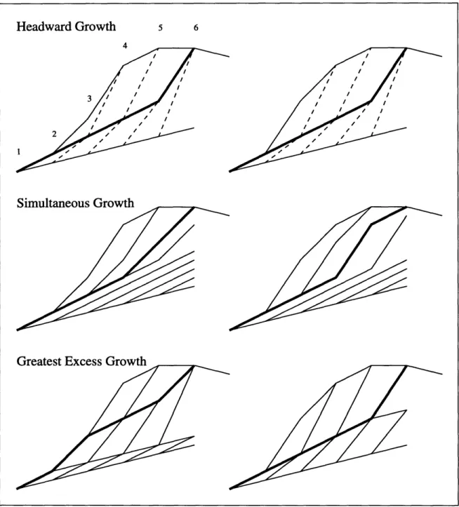
4 Sequencing of Erosion Events 4.1 Sequencing Variants . . . .

4.1.1 Headward Growth . . . 4.1.2 Simultaneous Growth .. 4.1.3 Random Growth . . . . 4.1.4 Greatest Excess Growth

23 24 28 31 36 38 41 43 44 47 49 49 52 55 57

4.2 Basin Morphology Implications . . . ... 4.3 Conclusions ...

5 A Comparison of Stability and Dynamic Equilibrium

5.1 Uplift in the Discrete Event Model . . . . 5.2 Flat Initial Conditions ... .. ...

5.3 Escarpment Retreat and Sloping Antecedent Conditions . . . . 5.3.1 Modes of Escarpment Retreat and Network Growth . . . . 5.3.2 Stationary Basin Forms ...

5.4 Summary ...

6 Influences of Storm Duration 6.1 General Framework ...

6.2 Prolonged Precipitation . . . . 6.3 Instantaneous Precipitation . . . . 6.4 Application Through the Discrete Event and 6.5 Implications for Basin Form . . . . 6.6 Conclusions ...

7 Conclusions

7.1 Summary of Results ... 7.2 Avenues for Further Study ...

Slope-Area Models 73 74 76 83 84 88 97 .. . 98 . . . 102 . . . 102 . . . 106 . . . 109 115 117 117 119

List of Figures

2-1 Schematic diagram showing three proposed modes of drainage network growth from Schumm et al. [37] ... 17

3-1 The development of topography by the Discrete Event model with an outlet specified in the corner ... 32 3-2 Topography and river networks as developed by (a) the Discrete Event

model and (b) the Slope-Area model . ... 35 3-3 Comparison of slope-area relationships for (a) the Discrete Event model

and (b) the Slope-Area model ... 37 3-4 Distribution of avalanche sizes and lifetimes from Bak et al. [4] for (a)

a 50x50 array, averaged over 200 samples, and (b) a 20x20x20 array, averaged over 200 samples ... 40 3-5 Distribution of avalanche (a) sizes and (b) lifetimes in the Slope-Area

model (from Ijjasz-Vasquez et al. [18]) . ... 45

4-1 Schematic diagram of three different erosion algorithms at work on two example slopes. Solid lines indicate slope profiles in between model iterations, whereas dashed lines indicate the changing profile shape during a single iteration. The bold line shows the profile when point 6 is captured . . . .. . 51 4-2 Snapshots during the erosion of a basin using (a) Headward Growth,

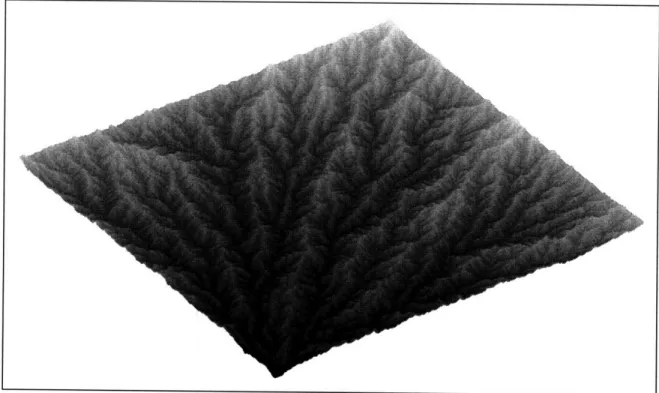
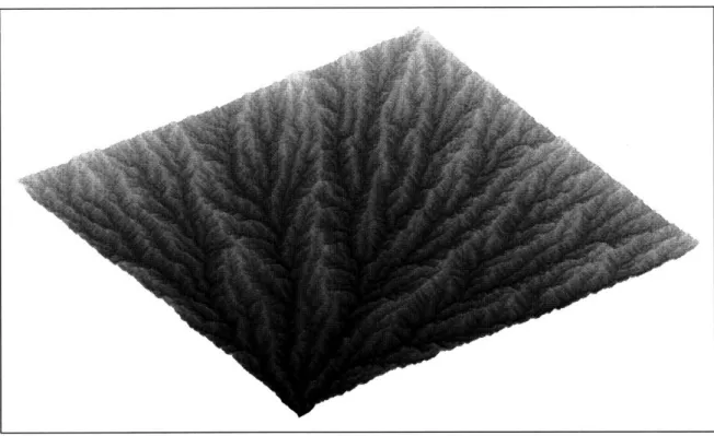
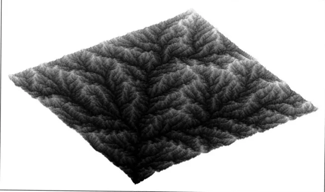
(b) Simultaneous Growth, (c) Random Growth, and (d) Greatest Ex-cess G rowth . . . 53 4-3 A basin developed by the Headward Growth variant ... 59

4-4 A basin developed by the Simultaneous Growth variant ... 60

4-5 A basin developed by the Random Growth variant . ... 60

4-6 A basin developed by the Greatest Excess Growth variant ... 61

4-7 Networks developed by the Discrete Event model variants ... 62

4-8 Distribution of drainage directions normalized by the outlet direction for a collection of runs of the four model variants . ... 64

4-9 Distributions of contributing area for basins developed by the Discrete Event model variants ... 65

4-10 Width functions for basins developed by the Discrete Event model variants . . . .. . 67

4-11 Slope-area relationships for basins developed by the Discrete Event m odel variants ... 69

4-12 Hypsometry for basins developed by variants of the Discrete Event model 70 5-1 Topography generated by the Discrete Event model with (a) Tcr = 0.01, U = 0, and K = 0.01, (b) Tr, = 0.005, U = 0.005, and K = 0.01, and (c) •r, = 0, U = 0.01, and K = 0.01. ... 79

5-2 Slope Area relations for stationary topographies generated with (a)Tr, = 0.01, U = 0, and K = 0.01, (b) T•r = 0.005, U = 0.005, and K = 0.01, and (c) r, = 0, U = 0.01, and K = 0.01. ... 80

5-3 Hack's Law for stationary topographies generated with (a),cr = 0.01, U = 0, and K = 0.01, (b) r,, = 0.005, U = 0.005, and K = 0.01, and (c) T•r = 0, U = 0.01, and K = 0.01. Solid line shows regressions, and dashed lines show slope of 1/2. . ... .. 81

5-4 Distribution of drainage directions for basins generated with (a) Tr = 0.01, U = 0, and K = 0.01, (b) -Tr = 0.005, U = 0.005, and K = 0.01, and (c) Tcr = 0, U = 0.01, and K = 0.01. ... 82

5-5 Snapshots during the evolution for the four cases where (a) and (b) include a non-zero critical shear and (c) and (d) include a positive uplift. (a) and (c) have initial surfaces sloping towards the baselevel whereas (b) and (d) have initial surfaces sloping away from the baselevel 86

5-6 Snapshots during the growth of the channels networks for Case 3 ... 87

5-7 Snapshots during the growth of the channels networks for Case 4. . . 89

5-8 Networks developed by the Discrete Event model where (a) and (b) include a non-zero critical shear and (c) and (d) include a positive uplift. (a) and (c) have initial surfaces sloping towards the baselevel whereas (b) and (d) have initial surfaces sloping away from the baselevel 91 5-9 Distribution of contributing areas for the four cases . ... 92

5-10 Hack's Law for the four cases ... 93

5-11 Distribution of drainage directions for the four cases ... 94

5-12 Slope-area relationships for the four cases . ... 95

6-1 Diagram of the discharge during a period of simulation ... 100

6-2 Diagram of the relationship between peak flow and contributing area for the long storm case ... 103

6-3 Diagram showing two basins with the same contributing area but dif-ferent peak flows after an instantaneous pulse of precipitation . . .. 104

6-4 Diagram showing peak flows for the instantaneous storm case . . .. 105

6-5 Correlation between contributing area and flow duration (or main stream length) using (a) a constant ruler length and (b) a ruler length that varies according to contributing area (solid lines show regressions) . . 111

6-6 Simulated basins where (a)-(c) have instantaneous precipitation and (d) has prolonged precipitation. Parameters are: (a) m = 1/2, n = 1, (b) m-= 1, n= 2, (c) m-= 2, n= 4, (d) m/n = 1/2 . ... 112

Chapter 1

Introduction

One of the fundamental principles of geomorphology is that the forms exhibited by topography reflect the processes that have been active in shaping that topography. This implies that river basin forms reflect climatic and tectonic forcing, the internal mechanics of erosion and other process, and to some extent previous basin forms and historical changes in the relevant processes.

Especially over the past ten years, a much greater understanding of the structure of river basins and channel networks has been achieved. This has in part been due to the widespread availability of digital elevation data. Such data has allowed the detailed analysis of many basins throughout the world. Another impetus was the introduction of fractals and scale invariance which has helped enrich the interpretation this data. The consistency of scale invariance between varied climatological and geological circumstances has hinted at new underlying aspects of basin evolution. Now, in addition to traditional geomorphological measures, fractal measures can be used to quantify natural topography and validate numerical models.

With the growing availability of data and interpretation techniques, quantitative modeling of river basins and topography in general has also expanded. Geomorphic modellers use the field data and simple conceptual arguments to construct their best quantitative understanding of the dynamics of basin evolution. In these models, we hope to capture the interplay between the internal dynamics, external forcing, and initial conditions that leads to the commonly observed forms of topography.

An expansive array of modeling approaches exist in geomorphology. Such nu-merical models include finite difference expressions of differential equations, cellular automata, and stochastic models based on fractals. The reasons for this diversity are the different interests and applications associated with many of these models. An-other cause is the stochastic nature of basin development and topography which limits validation techniques to statistical measures alone. However, it is often unclear how various models relate to one another and what each implies about the fundamental links between basin dynamics and form.

This work has one overarching goal. That is to investigate how various quan-titative descriptions of basin development affect the resulting basin geomorphology. This goal involves a comparison between the statistics of model simulations with well known characteristics of natural basins, and it includes a comparison between the model behavior with other published insights on the dynamics of basin evolution.

The first several chapters are dedicated to an introduction of the history of geo-morphological modeling and the general framework used in the analysis. Chapter 2 presents a literature review which attempts to summarize several of the main concep-tual and numerical models of basin evolution and channel network growth. Chapter 3 develops the model framework used throughout the rest of the analysis. This model is based on a description of shear stress and includes variants that encompass both a finite difference modeling approach and a discrete event approach. The model is quite similar to the one proposed by Rinaldo et al. [30] and to a lesser extent the one proposed by Ijjasz-Vasquez et al. [17]. Chapter 3 also makes some model compar-isons and discusses the relevance of the principle of Self-Organized Criticality (SOC) to geomorphological models.

The second set of chapters describe several experiments performed with the model developed in Chapter 3. Chapter 4 presents different possible dynamics of basin evolution which focus particularly on the mode of network growth and its affect on the resulting basin form. Four variants of the model are presented which are shown to approximate some of the classical conceptual models of channel network growth. Similar numerical models from the literature are also discussed.

The models in Chapter 4 approach a stationary condition termed stability which differs from dynamic equilibrium, another stationary condition reached by some ge-omorphological models. Either state may be achieved by some basins in nature. Chapter 5 investigates how the these conditions differ, and the effects of the initial conditions on topography approaching either state. This chapter has some relevance to escarpment retreat since the initial conditions that are considered include an overall slope towards or away from an specified or growing escarpment crest.

Chapter 6 examines the role that precipitation events play in basin evolution. It analytically develops the commonly used substitution of precipitation intensity times the contributing area for discharge. However, the case is derived under the condition of prolonged precipitation events. The chapter shows that an alternative case may also be derived in which precipitation arrives in instantaneous pulses. The implications of this theoretical change in climatic forcing on basin geomorphology is considered.

Chapter 2

Literature Review

It is the purpose of this chapter to provide some context for the analysis in the following chapters. The work to be presented draws from a wide variety of previous modeling studies as well as field and laboratory investigations. For the sake of brevity, only a few previous modeling efforts will be outlined here, and further discussion of relevant work will be included throughout the other chapters as applicable. The first section of this chapter considers some important conceptual and numerical models of channel networks. The second section considers some conceptual and numerical models of landscape evolution.

2.1

Channel Network Growth

Horton [14] was among the first to consider in detail how channel networks develop. A schematic diagram of his model is shown in part (a) of Figure 2-1 which is based on a similar diagram by Schumm et al. [37]. Horton suggested that parallel rills form quickly to drain an initially undissected slope. By chance, a certain rill which he termed the master rill carries more flow than the others, and with a higher discharge rate, this rill also has a greater incision rate. As the master rill incises, it exerts an influence on the surrounding rills. New areas are captured through a process of micropiracy, and the low relative elevation of the master rill causes flow in nearby territory to cross-grade and drain towards the master rill. Smaller side rills therefore

change their orientation to connect to the master rill and begin to form an organized network structure. According to Horton, such network growth can be seen on the slopes along the sides of highways.

Based on observations of channel network growth including those of Schumm [36]

in the badlands at Perth Amboy, New Jersey, Howard [15] proposed that networks grow in a headward fashion. In his view, a channel network grows as an intense "wave of dissection" progresses headward from an outlet to capture new territory. Once this wave has passed, a virtually complete channel network is left behind (see part (b) of Figure 2-1). This view differs from Horton's which regards the organization of channel networks as a product of readjustment of the initial pattern. Howard also proposed a set of related numerical models that describe this type of growth. Some of these models are simply topological, but others are simulated on a grid to include geometric limitations on channel growth. In one grid-based model, he first specifies some initial seeds or outlets. Then, at each iteration, one adjacent point on the grid is randomly selected for addition to the existing network. Several variants are also included in which the probabilities of branching and inactivity are explicitly controlled.

Glock [10] proposed a more complex conceptual model of growth than the ones considered by either Horton or Howard. Unlike Howard's model, Glock envisaged that channels of different sizes would progress headward at different rates during an extension phase of network growth. He expected the main channels to grow first in a stage he called elongation followed by the elaboration of the minor tributaries (see part (c) in Figure 2-1). Glock, however, also expected a reduction or integration of the network form. One case where this might occur (called abstraction) is when a smaller tributary disappears due to the lateral movement of a main stream. Glock allowed the possibility that the extension phase may coincide with the integration phase. His model is based on the interpretation of various mapped channel network forms.

Leopold and Langbein [24] and Shenck [19] suggested a model where channel networks grow by random walks. At the beginning of each iteration, a channel source is randomly placed somewhere on a grid. Then, the channel grows as the water flows

Reorganization

Headward Growth

/

Exten sion -El aboration

Figure 2-1: Schematic diagram showing three proposed modes of drainage network growth from Schumm et al. [37]

downstream from this point. At any point, it has equal probability of growing in each direction. The channel continues to develop until meeting an existing stream or region boundary, and loops are forbidden. While such a model develops fairly reasonable networks, its description of the dynamics of growth is probably now out-dated.

More recent network growth models have focused on the adaptation and testing of various cluster growth models. Stark [41] suggested that Invasion Percolation with self-avoidance may be an accurate method of simulating channel networks. In this model, a random strength is initially assigned to every link in a rectangular lattice. A single seed is specified which corresponds to the basin outlet. Then, at each iteration, the adjacent bond with the weakest strength is added to the growing network. Stark compares Invasion Percolation to the model of Howard [15] and determines that only Invasion Percolation obeys Hack's law.

Masek and Turcotte [26] propose Diffusion Limited Aggregation (DLA) as a model of channel network growth. In this model, first a seed is specified for the basin outlet, and then random walkers are introduced throughout the grid. These walkers move about until they either reach the edge of the simulation domain or meet the existing tree. When they meet the existing tree, the current location erodes to expand the network in that location. Masek and Turcotte suggest that the random walkers are similar to water parcels moving over an initially flat surface and eventually draining into the network.

In addition to the above models of channel network growth, two models of chan-nel network structure are worth mentioning. First is the classic idea of topologically random networks proposed by Shreve [39]. He first considered the population of topo-logically distinct networks all having the same number of links. Topotopo-logically distinct implies that no amount of stretching and rotating will transform one network shape into another. Shreve showed that the most probable configurations of these networks when their magnitude goes to infinity are those that give Horton's bifurcation ra-tio [14] near 4 (which lies well within the observed range). In addira-tion, if link lengths are randomly distributed then Horton's law of stream lengths [14] is also upheld with RL , 2 (again well within the observed range). Thus this theory explains the network

structure as the most probable configuration from a random population.

Rodriguez-Iturbe et al. [32] suggested an alternative view: "We believe that in an evolutionary system like the drainage network both chance and necessity should be operating; and, moreover, that the influence of necessity is felt through a tendency to minimize the total rate of energy expenditure in the network and the rate of energy per unit area of channel anywhere in the network." Along these lines, they proposed three principles of energy dissipation. The first principle states that energy is mini-mized in every link of the network. The second principle says that energy expenditure per unit area of channel is equal throughout the network. The third principle states that the energy in the network as a whole is minimized. Through a derivation de-scribed in detail in their paper, these principles amount to the minimization of energy expenditure E where:

E = EQ1/2Li. (2.1)

In this expression Q is discharge and L is the length of link i. Networks developed by minimizing energy expenditure have been shown to obey many statistical properties of real networks.

2.2

Landscape Evolution

In addition to the topological and two-dimensional modeling efforts described above, many authors have studied the three-dimensional dynamic form of rivers basins. In this section, a few of the classical perspectives and some of the most recent quantita-tive modeling approaches are described.

Davis [7] anticipated that topography progresses through a series of stages from youth, through maturity, to old age. At the beginning of his cycle of erosion, a brief period of rapid uplift raises the region above the baselevel. Over time, denudational processes wear down the landforms resulting in lower relief and a decline in slope angles. Without an interruption of renewed uplift, the landforms continue their decay until reaching a peneplain. A peneplain is defined as topography very near baselevel with subdued relief.

An alternative view has grown out of the work of Hack [12]. He proposed that after some time of denudation, topography reaches a state of dynamic equilibrium where the slopes are adjusted according to their lithological conditions and stream gradients are sufficient to carry their sediment loads. In this condition, he suggested, topography is uniformly lowered. Over time, this idea has been transformed to express an equilibrium where the addition of material to the system through tectonic uplift is balanced by the removal of material through denudational processes. Clearly this view differs from that of Davis since it implies a stationary state, and in the modern incarnation, suggests that uplift occurs over the same time scales as erosion. While both the models proposed by Hack and Davis are quite old, they still remain relevant interpretations of the geomorphological dynamics.

More recently, several numerical models have been developed which incorporate some of the ideas of Davis and/or Hack [21]. Here, only a few three dimensional models which include channel network growth are reviewed.

Willgoose et al. [49] and Tucker and Slingerland [45] analyzed transport-limited models. In transport-limited or alluvial channels, erosion is restricted by the capacity of the flow to carry weathered material. Therefore, the numerical simulations are controlled by the Exner continuity equation which states that the addition of elevation at a point is the uplift minus the increase in the carrying capacity in the downstream direction. The carrying capacity has the form Qm_Sn _{where Q is discharge, S is slope,}

and m and n are parameters. These models usually include diffusion to represent a suite of hillslope processes including tree throw, rheologic creep, and rainsplash.

An alternative set of landscape evolution models are detachment-limited models. In such models, erosion is assumed to be restricted by the detachment of material rather than its transport through the channels. These models apply to bedrock chan-nels and coarse-bed rivers. Now the change in elevation of a point is the uplift minus the erosion where the erosion rate has a similar form to the capacity above: QmS". Models of this type have been studied by Moglen and Bras [27], Tucker and Slinger-land [45], and Howard and Kerby [16]. Here again, diffusion is often used to simulate the relevant collection of hillslope processes.

A hybrid model which includes both detachment-limited and transport-limited conditions as special cases was developed by Kooi and Beaumont [20, 21]. In this model, it is assumed that the transport rate is not always at capacity. Instead, it takes some work to reach the transport capacity, or equivalently there is some erosion length scale. Detatchment-limited conditions arise when the carrying capacity is much larger than the material erodability, and transport-limited conditions arise when the erosion length scale goes to zero.

All of the above detachment-limited and transport-limited models involve the description of erosion using differential equations. However, alternative approaches have also been suggested. Chase [6] used cellular automata to describe the erosion process. In his model, precipitons are dropped at random locations on the simulation domain. When the precipiton lands, it causes some local erosion in the form of diffusion. Then the precipiton travels in the downslope direction, eroding at a rate proportional to the slope until reaching a carrying capacity which is proportional to the stream power. When carrying capacity is exceeded by a reduction in the surface slope, material is deposited according to specified rules.

A similar lattice model was proposed by Kramer and Marder [22]. In their nu-merical model (which differs from their analytical model), precipitation falls on the grid points at random intervals. At each site, both the water depth and the surface elevation are explicitly treated. If the water elevation differs between neighboring sites, water moves to reduce the difference, and for each unit of water that shifts, a corresponding unit of sediment is eroded if the neighbor's surface elevation is also lower.

Another lattice model was proposed by Leheny and Nagel [23]. In this model, precipitation again enters the model at a random site. The water then flows to a randomly selected downslope neighbor where the probability of selection is dependent on the elevation difference. All sites visited by a parcel of water are eroded by the same amount. Landsliding also occurs on the surface when the elevation difference between adjacent points exceeds a critical value.

pro-posed by Ijjasz-Vasquez et al. [17] and Rinaldo et al. [30]. The model propro-posed by Ijjasz-Vasquez et al. [17] is called the Slope-Area model and involves determining the basin configuration at dynamic equilibrium by enforcing the slope-area relation-ship [9, 11] at all points. The model developed by Rinaldo et al. [30] describes erosion as the culmination of discrete or episodic events. Both of these models will be con-sidered in greater detail in the following chapter.

2.3

Summary

As this review has shown, a great diversity of models has been used to simulate the development of channel networks and river basins. These models differ in the processes that are included (e.g. soil creep or landsliding) as well as their descriptions of the various processes. The main result found from an overview of these analyses is that aggregation patterns similar to those of natural river networks can be developed from a variety of approaches and that each of these approaches is able to match some of the observed characteristics. However, the link between the specified dynamics of the evolution and the resulting basin and network characteristics remains somewhat unclear. The next chapter develops a relatively broad framework through which some of the above models can be compared, and the following three chapters investigate the role that the erosional dynamics, initial conditions, and climatic and tectonic forcing play in determining the basin form.

Chapter 3

The Discrete Event Model

A wide variety of approaches has been utilized to model the evolution of river basins. One evolution model is the em Threshold model of Rinaldo et al. [30] and Rigon et al. [29]. This model attempts to describe the evolution of river basins from the per-spective of self-organization principles. It differs from many process-based evolution models because it includes a threshold below which erosion is ineffective and because it describes erosion as the culmination of discrete events rather than the continual movement of sediment.

This chapter describes a variant of the Threshold model which for clarity will be called the Discrete Event model. The next section develops the conceptual basis for the model which relies on a consideration of shear stress and highlights the differences between the model of Rinaldo et al. and the Discrete Event model. The second section discusses the algorithm through which the model is implemented. A comparison is made in the third section between the Discrete Event model and its cousin the Slope-Area model [17]. Finally, some comments are made regarding the self-organizing characteristics of these geomorphological models. In particular, can any of these models be considered a self-organized critical system as originally defined by Bak et

3.1

Conceptual Basis

Unfortunately, the mechanics of bedrock erosion remain poorly understood. However, three main processes are thought to drive the downwearing of bedrock beds: abrasion, plucking, and solution. Abrasion describes the affect of water and its sediment load as they flow or saltate across the bed surface. Over time, the impacts of the sediment load and the shear created by the flow wear down the bedrock. Plucking involves the removal of pieces of bedrock either by hydraulic lifting or the wedging of smaller material into the bedrock joints. Finally, solution describes chemical reactions that occur between the bedrock and the flow which break down the rock into new com-pounds that can be removed in the flow. The effectiveness of each of these processes will depend on the rock type, jointing characteristics, and climate. Additionally, in channels where the capacity to carry eroded material is small relative to the erosion rates (transport limited or alluvial channels), the material already in transport may limit the local erosion.

Considering only detachment limited channels, two of these processes, abrasion and plucking, depend in some way on the shear stress created by the flow over the rock surface. In addition, these two processes are expected to dominate under most combinations of rock type and climate. Thus, a reasonable model for bedrock channels is:

az

19t 0 otherwise

where z is the bed elevation, t is time, T is shear stress on the bed, Tr7, is a critical

shear stress, and kl and a are parameters. According to this equation, the elevation of the river bed is reduced only when the shear stress exceeds some critical value. This critical shear reflects the inherent strength of the bedrock and the degree of jointing. Once the shear exceeds this critical value, erosion occurs at a rate proportional to some power of the excess shear. The parameters controlling this rate, K1 and a, will

probably depend both on the material and the type of erosion.

evalua-tion of the processes, Trc* could be neglected and a f 1. By these assumptions, erosion is considered to be a smoothly operating process in time which depends nearly linearly

on the excess shear, and Equation 3.1 reduces to:

atOz_{= --k17}

(3.2)

since 7 > 0 by definition.

An alternate view was proposed by Rinaldo et al. [30]. They considered the threshold to be a critical component of erosion and the degree of nonlinearity to be severe. In this extreme, a -+ 0o, indicating that, when the critical stress is exceeded,

erosion occurs to abruptly reduce the shear stress directly to a critical value Tr,. Thus, erosion is not considered to be a smoothly acting process. Rather, it is a collection of discrete events, and Equation 3.1 reduces to a condition of stability:

T --- Tcr if

>cr

(3.3)

(3.3)

z= 0 otherwise

where Tr = T*'r + 1. The different critical shear stresses, -re and 7Tr, arise because as

a - oo00, (T - Tr)a goes to zero in Equation 3.1 when T - Tr < 1.

To evaluate this condition of stability at all locations and times, one requires some additional information to determine the dependence of shear stress on the existing topography. The boundary shear stress created by steady uniform flow can be written:

T = pgRS (3.4)

where p is density of water, g is the acceleration of gravity, R is hydraulic radius, and S is the slope. Notice that under the condition of steady uniform flow, the bed slope, friction slope, and water surface slope are equivalent.

The hydraulic radius will vary systematically throughout any given channel net-work. This dependence can be understood by considering three additional relations.

First, for a wide channel, hydraulic radius can be related to the discharge Q as:

R = Q (3.5)

vb

where v is the cross-sectionally averaged flow speed and b is the channel width. Sec-ond, the Darcy-Weisbach Equation describes the average flow speed as a function of the geometry and a friction factor f:

v =

.8R

(3.6)

f

Third, observations by Leopold and Maddock [25] show a dependence of channel width on discharge rate as one moves along a channel network. The resulting empirical relation is:

b = k2Q6 (3.7)

where k2 is a coefficient, and 6 P 1/2. Given these three relations, the hydraulic radius can be written in terms of discharge and slope:

R = Q2(1-6)13S-1/3 (3.8)

Substituting this relationship for the hydraulic radius into the expression for shear stress, one finds that:

7 = kQmSn (3.9)

where k = pg [f/ (8gk2)]1/3, m = 2(1 - 6)/3

#

It should be noted that Rinaldo et al. [30] use a different methodology to derive the dependence of hydraulic radius on slope and discharge. They assume directly that:

R = k

Q

(3.10)

where k3 is a coefficient and m - 1/2. As will be shown below, slope depends on discharge at the stability threshold, and a similar relation between hydraulic radius

and discharge results from the approach using the Darcy-Weisbach equation above. Using the Rinaldo et al. [30] derivation, Equation 3.9 still holds, however, k = pgk3, m ? 1/2, and n = 1. Because the exact values of the coefficient and exponents depend on the assumptions, the general form of Equation 3.9 will be used in the following discussion, but no specific parameter values will be endorsed.

In order to complete the model, it remains necessary to describe the variation of discharge in terms of the topography. The simplest approach is to assume that discharge increases linearly with increasing upstream area or:

Q = PA (3.11)

where P is the characteristic effective precipitation intensity (where effective precip-itation indicates the precipprecip-itation that becomes runoff) and A is contributing area. Obviously, this parameterization is extremely simple, and further analysis regarding this point is performed in Chapter 6 where an alternative (simple) hydrologic model is developed and compared with this approach.

Substituting for discharge in the description of hydraulic radius, and then substi-tuting this into the relationship for shear stress, one finds:

T = KA'm_{S" (3.12)}

where K - kPm . Now the condition for stability, previously written in terms of shear, can also be written in terms of slope. Given an existing channel configuration and the associated contributing areas:

Scr = )" A-_m/" . _(3.13)

Notice that the two approaches described above supply differing m and n values but the same m/n value. The numerical evaluation of Equation 3.13 is at the heart of the Threshold and Discrete Event models.

effects of erosion is also perturbed by adding elevation to randomly selected loca-tions. The justification of this approach relies on the notion of energy minimization. Rodriguez-Iturbe et al. [32] have proposed that river networks develop under three principles of energy minimization, and networks simulated according to these rules have been shown to strongly resemble existing networks. Rinaldo et al. [30] have shown that by perturbing a network developed by the above erosion model, lower states of energy expenditure are achieved. However, their analysis has also shown that the reduction in energy due to such perturbations is strongly dependent on the selected initial conditions.

In this analysis, the use of perturbations will be avoided because their physical meaning is unclear. It is known that the perturbations help the model achieve lower states of energy expenditure, but the efficiency with which real river networks are able to minimize energy and the relationship of the efficiency to the perturbations is an unresolved question. Therefore, this analysis will not employ perturbations and will avoid using the particular initial conditions where the effects of these perturbations are significant (i.e. conditions which begin with many stable points and an unrealistically developed river network).

In addition, Rigon et al. [29] have extended the Threshold model to include the effects of diffusive hillslope processes. Because hillslopes are not the focus of this analysis, this aspect of the extended model will also be neglected here. It should be noted, however, that the spatial discretization used for numerical simulations intro-duces some numerical diffusion which plays an important role (see below). The next section describes the numerical application of the model derived above.

3.2

Summary of Model Algorithm

Before applying the Discrete Event model, the domain of simulation must be specified along with boundary and initial conditions. The model is applied on a rectangular grid and the domain can be any selected shape. The boundaries are fixed in location and elevation and do not allow flow to pass in or out of the domain. For initial conditions,

the model only requires that the flow directions are well defined at all locations. This implies that adjacent elevations must not have identical elevations. Published initial conditions [30, 29] include antecedent river networks (realistic and unrealistic) and nearly constant elevations with some superimposed, uncorrelated noise.

Additionally, any number of outlets can be specified. An outlet is simply a point with significantly lower elevation than the rest of the region. Physically, a single outlet may correspond to the head of a pre-existing, deeply incised channel at the region's edge; lines of outlets roughly represent an escarpment edge. Because outlets are much lower then the rest of the domain, they will tend to capture the flow from a large portion or all of the region depending upon their number, locations, and elevations. However, in all other respects, outlets behave the same as any pit on the topography. Once the initial and boundary conditions are defined, simulation may begin. As described above, the model is rule-based rather than rate-based, and can therefore be most easily described algorithmically:

1. Determine drainage directions. Water and sediment are assumed to flow from a given point deterministically in the direction of steepest decent. However, because the model operates on a grid, this vector must be mapped towards one of the point's neighbors. In this analysis, the eight nearest neighbors will be consider valid flow directions, but four or even sixteen neighbors may also be used. The simplest procedure to assign a flow direction is to route the flow towards the neighbor which forms the steepest slope with respect to the current point. Thus the drainage direction for a node i,j on the lattice is assigned towards zdwn where zdon satisfies:

dozwni ,j sti+ie

= Max, i li,+ ii = -1, 0,1 jj = -, 0,1 (3.14)

where the indices ii, jj indicate relative locations of the nearest eight neighbors and Al is the horizontal distance between i, J and i+ii, j+jj. Rinaldo et al. [30] use Al = constant in all directions. In this case, the above maximization reduces to the selection of the neighbor with the lowest elevation. Here, we

instead maintain lattice geometry, and the distances of the diagonal directions will be V12 times the principal directions. Since, by definition of the grid, all neighbors are not equally distant from the point, anisotropy will be introduced no matter which approach is taken. Conditions for isotropy have recently been studied in the context of cellular automata models of lattice gases by Rothman and Zaleski [33].

2. Determine contributing areas. Because unique flow directions are known at all locations, the area contributing to the flow at any grid point is also known. A given point is assumed to drain its own grid cell and all of those draining through it.

3. Select sites for adjustment. Now that the configuration of the existing networks are known, any locations where the shear stress exceeds the critical value can be identified. At any given iteration of the simulation, some proportion or all of these points must be selected for elevation adjustment due to erosion. Rigon et al. [29] select only the point with the greatest excess shear for adjustment. Alternatives to this approach will be considered in detail in the next chapter.

4. Erode the selected unstable points. When a point is eroded, its elevation is immediately reduced to a value which brings about minimal stability, where minimal stability means r = Tcr or S = Scr. The slope at a grid point i,

j

( Zdown

Sij = z i j -

(3.15)

Because Al is finite, some numerical diffusion is introduced into the simulations. This diffusion plays an important role since it causes the attenuation of baselevel changes as they propagate upstream.

The elevation at the point after erosion (ziw•) can be set from Equation 3.13:

Note that there are effectively two parameters in this model: a coefficient and an exponent on A. The coefficient controls the vertical scale of the topography, and the exponent controls the overall concavity (and affects the network structure). Elevations are always decreased by the adjustments so that this equation forms an upper bound on the elevation of a point with a given contributing area. The sequencing and number of adjustments may be important since zdown and A will potentially change due to the erosion of points in the vicinity of i, j.

5. Repeat the process. The process of characterizing the existing basin and adjust-ing elevations is repeated until no point in the basin is unstable. The growth occurs because of two main feedback mechanisms in the model. First, as a point is reduced in elevation, points upstream may now find themselves with much higher relative elevations (or steeper slopes) than stability allows. This new instability will require a reduction in their elevations as well. Second, if a point is reduced in elevation, it may become the downstream neighbor for new points and capture additional contributing area. If the point drains a greater area, it will find itself unstable again since larger contributing areas require flatter slopes for stability. Thus, by either mechanism, the erosion of one point may propagate to affect larger regions of the domain.

An example of the growth of a river basin by this model is shown in Figure 3-1. In this application, an outlet is specified in the lower left corner of the basin and is sufficiently low to eventually capture the entire domain. Growth occurs principally but not exclusively headward from this location.

3.3

Comparison with the Slope-Area Model

The description of landscape evolution presented above is also quite similar to the Slope-Area model proposed by Ijjasz-Vasquez et al. [17]. This section compares the two models.

Figure 3-1: The development of topography by the Discrete Event model with an outlet specified in the corner

by Moglen and Bras [27] and Tucker and Slingerland [45]. They consider landscapes which develop under the competition between uplift and erosion by bedrock channels. Erosion in this approach is assumed to depend on slope and area each to some power, a form which can be derived from a consideration of shear stress as shown above with Tr = 0. Neglecting any term reflecting diffusive processes, their model can be written:

Oz

a= U - _AmSn

(3.17)

where U is uplift, 3, m, and n are parameters. At equilibrium az/at = 0, so the

slope can be found in terms of the contributing area:

Seq

=

A-

_.

_(3.18)

Note that a similar relationship also arises from transport limited models. On a discrete grid as described above, one can solve for the elevation at a point i, j:

new down 1/n -m/n(3.19)

zij, = ZiJ + Alij ij (3.19)

The Slope-Area model employs Equation 3.19 to develop the landscape. Like the Discrete Event model described above, the Slope-Area model has essentially two parameters: a coefficient of A which controls the vertical scale of the topography and an exponent on A which affects the concavity and network structure. At every iteration, drainage directions and contributing areas are determined at all locations on the network, and elevations of all points are adjusted according to Equation 3.19 to enforce a slope-area relationship. Again, the order in which the adjustments are made plays a significant role in the model (see Chapter 4). Any initial conditions that provide well defined drainage directions can be selected.

Clearly similarity is expected in the resulting topographies because of the similar-ity between Equation 3.19 and Equation 3.16. Both equations essentially enforce the slope-area relationship throughout the basin development, but they do so for different reasons and in a slightly different manner. The Slope-Area model can either raise or

lower points to enforce this relationship because it describes the competition between uplift and erosional processes. Thus, its final state is an equilibrium where the effects of these processes exactly balance. The Discrete Event model can only lower the elevation of points since it describes only the effects of erosion on bedrock without uplift or deposition. Thus, its final state is one characterized by the stability of all points rather than dynamic equilibrium, and the vertical dimension of the topogra-phy is determined by T7r

$

Another important conceptual difference exists between the two models. The Dis-crete Event model is proposed as a physical description of the process of bedrock erosion without uplift. Thus, transient states which occur during the evolution are interpreted as phases of physical evolution to the extent that this model represents re-ality. In contrast, the Slope-Area model, only has physical meaning for the final state where the system reaches equilibrium. Before this state, the series of intermediate topographies must be considered as merely trial solutions.

Figure 3-2 shows a visual comparison between basins developed by the Discrete Event model and the Slope-Area model (top and bottom of the figure, respectively). Both basins began with the same initial and boundary conditions so that these two topographies differ only because the lower one allows the increase of elevations to enforce the Slope-Area relationship. This figure shows that these two topographies are different. One would expect that the networks will differ some in appearance be-cause some small differences in elevations that occur during the growth may reroute channels and slightly alter the network structure. However, some systematic differ-ences are visible. In particular, confludiffer-ences tend to occur further upstream for basins developed by the Slope-Area model than for those from the Discrete Event model. This observation is confirmed by an examination of energy expenditure for the two types of basins. In general, Slope-Area basins on a 100x100 pixel grid have about 5 percent less energy expenditure than their corresponding Discrete Event basins.

Figure 3-3 shows the Slope-Area relationships for both basins. At small contribut-ing areas, the Discrete Event model leaves some points below their critical slopes.

a1

-c

-4

Topography and river networks as developed by (b) the Slope-Area model

Because the elevations of all points were reduced during evolution, these points were once at their critical slopes. However, reduction in their contributing areas by alter-ations in the channel network left these points well below their critical values. In other geomorphic characteristics such as exceedance probability distribution of contributing areas, hypsometry, and width functions these two basins appear quite similar.

3.4

Self-Organized Criticality

Fractal structures and power law scaling have been recognized in a large number of natural systems. The commonality of such characteristics indicates that power laws inherently result from the dynamics of many complex systems without detailed spec-ification of the conditions. However, a physical understanding of how such properties arise remains an important question in the study of fractal phenomena. As Bak et al. [3] write, "The grand and general question is how the laws of physics-which describe processes on the microscopic scale-can lead to a world organized on all scales."

One step in the investigation of this question has been the notion of Self-Organized Criticality (SOC) as proposed by Bak et al. [4, 5]. They suggest that fractal charac-teristics occur so commonly in natural systems because these systems are attracted under a broad range of initial and boundary conditions to critical states. As observed previously in the literature [5], critical states such as phase transitions imply that small perturbations can have influence over a wide range of spatial and temporal scales.

This section investigates the idea of SOC and its relevance to geomorphology where power laws are extremely common. In the first subsection, the characteristics that are observed at the self-organized critical state are summarized. Then, in the following subsection, an overview of the current debate on the self-organized critical nature of geomorphic models is presented. The position of Sapozhnikov and Foufoula-Georgiou [34] is summarized first. In their view, the current set of geomorphic models does not display SOC. A counter argument by Ijjasz-Vasquez et al. [18] is then

pre-Discrete Event model 0 a) . 1 --o 10 -W/ 10-2 100 101 102 103 104

Contributing Area (pixels)

Figure 3-3: Comparison of slope-area relationships for (a) the Discrete Event model and (b) the Slope-Area model

'U S10 -2

II

1 rl

1rl

7 r

(

I

iiI.

.

sented. In their view both the Slope-Area model and the Threshold model would be viewed as self-organized critical. Because this debate is not central to the rest of the work presented in this document, the arguments are merely summarized for completeness, and neither position is endorsed.

3.4.1

Characteristics of Self-Organized Criticality

To illustrate the SOC idea, consider Bak's sandpile model first in one dimension. A simulation region of length N is defined which, for example, is initially devoid of sand. The left boundary is closed, but the right boundary allows the sand to leave freely. The sandpile is characterized by height differences (or slopes since the grid is regularly spaced) h where hi - zi - zi+l and z is the height at a point i. Over time, grains of sand are dropped at random locations in the domain. If a grain is dropped at point i, this implies:

h2 -- hi + 1

(3.20) hi-1 •-- hi-1- 1

which is simply an increase of zi by one. When the slope at a point exceeds a critical value her, an avalanche occurs which redistributes the mass as:

hi - hi - 2 (3.21)

hi±1 hi+1 + 1.

This simply moves the excess material down the slope to the right. The adjacent right point may now exceed its critical slope; if so, it would be readjusted in the same manner. Such avalanching occurs until all points are stable. her should not be considered a parameter since the SOC behavior does not arise under any tuning of this value.

As time progresses, the sandpile will increase to the state where all locations are at their critical slopes. This is the minimally stable state since sand added to any point will be unstable and fall straight out of the pile at the right boundary. Thus, the scale of the avalanches is infinite, and the dynamics are trivial.

Now consider a 2-D case. The addition of a sand grain in the i, j domain is defined as:

hij-1 - hi,j- 1 - 1 (3.22)

hij ~ hi,j + 2

In this case, h represents the slope in the (+i, +j) direction. When hcr is exceeded, avalanching occurs:

hij -- hij - 4

hi*, - hi±l,j + 1 (3.23)

hij±l-+ hi,j±₁ + 1

which represents the shifting of material in the i + 1, j and i, j + 1 directions if the smaller effects on hi+l,j-1 and hi_1,j+l are neglected. The model can also be viewed as two dimensional nonlinear diffusion.

This model also reaches a stationary state but one with more interesting dynam-ics (viz. SOC). Here, not all points are at their critical slope; instead, the system is attracted to a condition where only a fraction of the points are minimally stable with the the rest more-than-stable. Since the more-than-stable points dampen per-turbations, avalanches can therefore be of varying sizes and durations. The size of an avalanche is measured as the number of points where mass is redistributed from a single perturbation, and the lifetime is the number of iterations over which such redis-tribution occurs. At the critical state, the avalanches are observed to be distributed as a power law in size and lifetime (Figure 3-4).

Variations on this model have also been investigated by Bak and others [5]. Some cases include: initial conditions well above or below the threshold h,, and closed or open boundaries. Under a broad set of conditions, the model will self-organize to a critical state.

So what characteristics of this model are required to develop SOC? This is not known exactly and represents an area of active research, but clear examples of SOC share the following characteristics: extended spatial degrees of freedom in which the system operates, two or more dimensions, and a process which is active up to a

C C C ! , II Y C 10' i0 10" 10, .0' 10' t S

Figure 3-4: Distribution of avalanche sizes and lifetimes from Bak et al. [4] for (a) a 50x50 array, averaged over 200 samples, and (b) a 20x20x20 array, averaged over 200 samples

40 U

threshold.

Since the purpose here is to examine whether existing landscape evolution models display SOC states, the section only attempts to define the characteristics that mark the behavior of an SOC system. The principal characteristics fall directly out of the terminology.

* The SOC state is an attractor over a broad range of parameter values and initial and boundary conditions. It follows that once reaching SOC, a system never leaves this state (which implies that the state is stationary). Bak et al. [5] confirm this characteristics, "By self-organized we mean without detailed speci-fication of initial conditions and robust with respect to variation in parameters."

* SOC also requires criticality, implying that perturbations can propagate over all length and time scales. Alternatively, in the words of Bak et al. [5], "The dy-namical process creates a stationary state where transport takes place through events on all length scales and time scales."

* The SOC state does not correspond to the minimally stable state, and more-than-stable points play a key role in the system's behavior. These points limit the extent of avalanches and help develop the "punctuated equilibrium" of SOC where catastrophic events of varying size pull the system away from criticality while the noise slowly pushes the system back to this state.

Using this rough definition, the geomorphic models described above can be evaluated to determine whether the ensuing power laws might derive from SOC. The next section summarizes an analysis of Sapozhnikov and Foufoula-Georgiou [34] that investigates whether the perturbation approach of the Rinaldo et al. [30] model is truly SOC.

3.4.2

Does the Threshold Model Exhibit SOC?

Many authors have claimed that they observe SOC in their geomorphic models [41, 17, 43, 30], however, none have presented a definitive demonstration of canonical SOC behavior. Upon first glance the Rinaldo et al. [30] model is clearly worth examining as

a possible example of SOC in a geomorphological context. In particular, it includes a process which operates up to a threshold, creating a system with a collection of points at barely stable and more than stable states. Furthermore, it demonstrates many of the power laws that are observed in natural basins.

Sapozhnikov and Foufoula-Georgiou [34] have examined whether the Threshold model exhibits SOC behavior. They adopt a similar description of SOC as that described above. Specifically, they observe that the SOC state is (1) critical and demonstrates power law scaling in the impacts of perturbations in space and time and (2) attracted to the critical state. The state they examine for SOC is the state after the initial growth of the model where all points lie below the critical shear stress. According the approach of Rinaldo et al. [30], this state is perturbed by adding elevation to a node and then allowing the system to re-adjust the elevations to enforce the critical shear stress condition.

Two important differences can be observed between this model and canonical SOC. First, power law scalings do not always hold in this state. Specifically, Rinaldo et al. [30] begin a simulation with a comb-like river network in which all points are stable, but the system does not display power law scaling until the final state when perturbations no longer affect the state of the system. Second, the system is not in a stationary state. As the perturbation/relaxation process advances, the power laws develop indicating a statistical change in the system. These two differences are important since they contradict the observed characteristics of SOC given above.

Additionally, Sapozhnikov and Foufoula-Georgiou [34] argue that the final config-uration (once fractal scaling has developed) cannot be considered SOC as it violates the condition of a punctuated equilibrium. In this state, the elevations remain un-changed. Although this is a specific case of stationarity, there can obviously be no scaling in the lifetime or size of the impacts of perturbations. Thus, Sapozhnikov and Foufoula-Georgiou [34] conclude that no state of the system corresponds to the SOC state demonstrated by the sandpile model.