HAL Id: hal-03083517
https://hal.archives-ouvertes.fr/hal-03083517
Preprint submitted on 19 Dec 2020
HAL is a multi-disciplinary open access
archive for the deposit and dissemination of
sci-entific research documents, whether they are
pub-lished or not. The documents may come from
teaching and research institutions in France or
abroad, or from public or private research centers.
L’archive ouverte pluridisciplinaire HAL, est
destinée au dépôt et à la diffusion de documents
scientifiques de niveau recherche, publiés ou non,
émanant des établissements d’enseignement et de
recherche français ou étrangers, des laboratoires
publics ou privés.
Chessel
To cite this version:
Minh Phan, Katherine Matho, Emmanuel Beaurepaire, Jean Livet, Anatole Chessel. nAdder: A
scale-space approach for the 3D analysis of neuronal traces. 2020. �hal-03083517�
nAdder: A scale-space approach for the 3D analysis of neuronal traces
Minh Son Phan1, Katherine Matho2, Emmanuel Beaurepaire1, Jean Livet2, and Anatole Chessel1 1Laboratory for Optics and Biosciences, CNRS, INSERM, Ecole Polytechnique, IP Paris, Palaiseau, France
2Sorbonne Université, INSERM, CNRS, Institut de la Vision, 17 rue Moreau, F-75012 Paris, France
December 4, 2020
1
A
BSTRACTTridimensional microscopy and algorithms for automated segmentation and tracing are revolutionizing
2
neuroscience through the generation of growing libraries of neuron reconstructions. Innovative
3
computational methods are needed to analyze these neural traces. In particular, means to analyse the
4
geometric properties of traced neurites along their trajectory have been lacking. Here, we propose
5
a local tridimensional (3D) scale metric derived from differential geometry, which is the distance
6
in micrometers along which a curve is fully 3D as opposed to being embedded in a 2D plane or 1D
7
line. We apply this metric to various neuronal traces ranging from single neurons to whole brain data.
8
By providing a local readout of the geometric complexity, it offers a new mean of describing and
9
comparing axonal and dendritic arbors from individual neurons or the behavior of axonal projections
10
in different brain regions. This broadly applicable approach termed nAdder is available through the
11
GeNePy3D open-source Python quantitative geometry library.
12
Keywords Computational neuroanatomy · connectomics · 3D neuronal reconstructions · axonal and dendritic arbors ·
13
scale space · quantitative geometry · Python
14
1
Introduction
15
Throughout the history of the field of neuroscience, the analysis of single neuronal morphologies has played a major
16
role in the classification of neuron types and the study of their function and development. The NeuroMorpho.Org
17
database (Ascoli,2006;Ascoli et al.,2007), which collects and indexes neuronal tracing data, currently hosts more than
18
one hundred thousand arbors of diverse neurons from various animal species. Technological advances in large-scale
19
electron (Helmstaedter et al.,2013;Kasthuri et al.,2015;Motta et al.,2019) and fluorescence microscopy (Gong et 20
al.,2013;Winnubst et al.,2019;Abdeladim et al.,2019;Wang et al.,2019;Muñoz-Castañeda et al.,2020) facilitate
21
the exploration of increasingly large volumes of brain tissue with ever improving resolution and contrast. These
22
tridimensional (3D) imaging approaches are giving rise to a variety of model-centered trace sharing efforts such as the
23
MouseLight (http://mouselight.janelia.org/,Winnubst et al.,2019), Zebrafish brain atlas (https://fishatlas.neuro.mpg.de/,
24
Kunst et al.,2019) and drosophila connectome projects (https://neuprint.janelia.org/,Xu et al.,2020), among others.
25
Corresponding author: Anatole Chessel, anatole.chessel@polytechnique.edu
.
CC-BY-NC 4.0 International license
available under a
(which was not certified by peer review) is the author/funder, who has granted bioRxiv a license to display the preprint in perpetuity. It is made The copyright holder for this preprint this version posted December 4, 2020.
;
https://doi.org/10.1101/2020.06.01.127035
doi: bioRxiv preprint
Crucially, the coming of age of computer vision through advances in deep learning is offering ways to automate the
26
extraction of neurite traces (Magliaro et al.,2019;Januszewski et al.,2018;Radojevi´c & Meijering,2019), a process
27
both extremely tedious and time consuming when performed manually. This is currently resulting in a considerable
28
increase in the amount of 3D neuron reconstructions from diverse species, brain regions, developmental stages and
29
experimental conditions, holding the key to address multiple neuroscience questions (Meinertzhagen,2018). Methods
30
from quantitative and computational geometry will play a major role in handling and analyzing this growing body
31
of neuronal reconstruction data in its full 3D complexity, a requisite to efficiently and accurately link the anatomy
32
of neurons with varied aspects such as their function, development, and pathological or experimental alteration.
33
Furthermore, morphological information is of crucial importance to address the issue of neuronal cell type classification,
34
in complement to molecular data (Bates et al.,2019;Adkins et al.,2020).
35
An array of geometric algorithmic methods and associated software has already been developed to process neuronal
36
reconstructions (Bates et al.,2020;Cuntz et al.,2010;Arshadi et al.,2020). Morphological features enabling the
37
construction of neuron ontologies, described for instance by the Petilla convention (Petilla Interneuron Nomenclature 38
Group et al.,2008), have been used for machine learning-based automated neuronal classification (Mihaljevi´c et al.,
39
2018). These features have also been exploited to address more targeted questions, such as comparing neuronal arbors
40
across different experimental conditions in order to study the mechanisms controlling their geometry (Santos et al.,
41
2018). In the context of large-scale traces across entire brain structures or the whole brain, morphological measurements
42
are employed for an expanding range of purposes, e.g. to proofread reconstructions (Schneider-Mizell et al.,2016),
43
probe changes in neuronal structure and connectivity during development (Gerhard et al.,2017) or identify new neuron
44
subtypes (Wang et al.,2019).
45
So far however, metrics classically used to study neuronal traces tend to rely on elementary parameters such as length,
46
direction and branching; as such, they do not enable to finely characterize and analyze neurite trajectories. One
47
particularly interesting parameter that characterizes neurite traces is their local geometrical complexity, i.e. whether they
48
adopt a straight or convoluted path at a given point along their trajectory. This parameter is of particular relevance for
49
circuit studies, as it is tightly linked to axons’ and dendrites’ assembly and their role in information processing: indeed,
50
axons typically follow simple paths within tracts while adopting a more complex structure at the level of terminal arbor
51
branches that form synapses. Moreover, the sculpting of axonal arbors by branch elimination during circuit maturation
52
can result in convoluted paths (Keller-Peck et al.,2001;Lu et al.,2009). The complexity of a neurite segment thus
53
informs both on its function and developmental history. Available metrics such as tortuosity (the ratio of curvilinear to
54
Euclidean distance along the path of a neurite) are generally global and average out local characteristics; moreover,
55
traces from different neuronal types, brain regions or species can span vastly different volumes and exhibit curvature
56
motifs over a variety of scales, making it difficult to choose which scale is most relevant for the analysis. One would
57
therefore benefit from a generic method enabling to analyze the geometrical complexity of neuronal trajectories 1)
58
locally, i.e. at each point of a trace, and 2) across a range of scales rather than at a single, arbitrary scale.
59
Methods based on differential geometry have been very successfully applied in pattern recognition and classic computer
60
vision (Sapiro,2006;Cao,2003). In particular, the concept of scale-space has led to thorough theoretical developments
61
and practical applications. The key idea is that starting from an original signal (an image, a curve, a time series, etc.),
62
one can derive a family of signals that estimate that original signal as viewed at various spatial or temporal scales. This
63
enables to select and focus the analysis on a specific scale of interest, or to remove noise or a low frequency background
64
signal; in addition, scale-space analysis also provides multi-scale descriptions (Lindeberg,1990). On 2D curves, the
65
mean curvature motion is a well-defined and broadly applied scale-space computation algorithm (Cao,2003). So far,
66
however, comparatively little has been proposed concerning 3D curves, such data being less common (Digne et al.,
67
2011). Applications of curvature and torsion scale-space analyses for 3D curves have been reported (Mokhtarian,1988)
68
but remain few and preliminary; the inherent mathematical difficulty represents another reason for this gap. Neuronal
69
trace analysis clearly provides an incentive for further investigation of the issue.
nAdder: A scale-space approach for the 3D analysis of neuronal traces
Here, we present a complete framework for scale-space analysis of 3D curves and applied it to neuronal arbors. This
71
method, which we name nAdder for Neurite Analysis through Dimensional Decomposition in Elementary Regions,
72
allows us to compute the local 3D scale along a curve, which is the size in micrometers of its 3D structure, i.e. the size
73
at which the curve locally requires the three dimensions of space to be described. This scale is quite small for a very
74
straight trace, and larger when the trace displays a complex and convoluted pattern over longer distances. We propose
75
examples and applications on several published neuronal trace datasets that demonstrate the interest of this metric to
76
compare the arbors of individual neurons, extract morphological features reflecting local changes in neurite behavior,
77
and provide a novel region-level descriptor to enrich whole brain analyses. Implementation of the nAdder algorithms
78
along with an array of geometry routines and functions are made available in the recently published GeNePy3D Python
79
library (Phan & Chessel,2020), available at https://genepy3d.gitlab.io. Code to reproduce all figures in this study,
80
exemplifying its use, is available at https://gitlab.com/msphan/multiscale-intrinsic-dim.
81
2
Results
82
We introduce a new form of analysis to investigate the spatial complexity of neuronal arbors. Our approach consists of
83
decomposing each branch of a neuronal arbor into a sequence of curve fragments which are each assigned an intrinsic
84
dimensionality, i.e. the smallest number of dimensions that accurately describes them, from which we compute a local
85
3D scale, defined as the highest scale at which the curve locally has a 3D intrinsic dimensionality. The first sub-section
86
of the Results details the principle underlying this approach. We next demonstrate its purpose, accuracy and relevance
87
through several applications.
88
2.1 Computation of the local 3D scale of neuronal traces from their multiscale intrinsic dimensionality
89
Given a neuronal arbor, we decompose each of its branches into a sequence of local curved fragments, which are
90
classified according to their intrinsic dimensionality, defined by combining computations of both curvature and torsion
91
of the curves. Briefly, a portion of curve with low torsion and curvature would be considered a 1D line, one with high
92
curvature but low torsion would be approximately embedded within a 2D plane, and a curve with high torsion could only
93
be described by taking into account the three spatial dimensions. This results in a hierarchical decomposition, capturing
94
the fact that a 1D line is basically embedded in a 2D plane (Figure 1A, S1). To validate the proposed decomposition,
95
we applied it on simulated traces presenting different noise levels. Our algorithm reached accuracies above 90% with
96
respect to the known dimensionality of the simulations at low noise level and still above 80% at high noise level, while
97
an approach not based on space-scale which we took as baseline (Yang et al.,2016;Ma et al.,2017) was strongly
98
affected by noise (Figure 1A, S2 and S3; details on the simulation of traces, noise levels and algorithm are available in
99
the Methods section).
100
Our proposed decomposition of traces according to their local intrinsic dimensionality depends on the scale at which the
101
analysis is performed. To develop a metric based on this decomposition that would be robust to scale, we implemented
102
a space-scale approach. The notion of scale can be abstractly interpreted as the level of detail that an observer takes
103
into account when considering an object, varying from a high level (when observing a trace up close i.e. at smaller
104
scales), to low level (when observing it from afar i.e. at larger scales). A scale-space is the computation of all versions
105
of a given curve across spatial scales. Several mathematical and computational frameworks have been proposed to
106
compute such ensemble of curves; the simplest one used here consists of smoothing the initial portion of trace analyzed
107
by convolutions of its coordinates with Gaussian kernels. The dimensionality of such a curve element, as we analyze it
108
at increasing scales, is typically best described as 3D at the smallest scales (i.e. taking in account a high level of detail),
109
and becomes 2D or 1D at larger scales (i.e. low level of detail) as more and more details are smoothed out (Figure 1B,
110
middle panel and S4). Here, in the context of neuronal arbors, scales are measured in micrometers, by computing the
111
radius of curvature of the smallest detail kept at that scale (see methods for details).
112
.
CC-BY-NC 4.0 International license
available under a
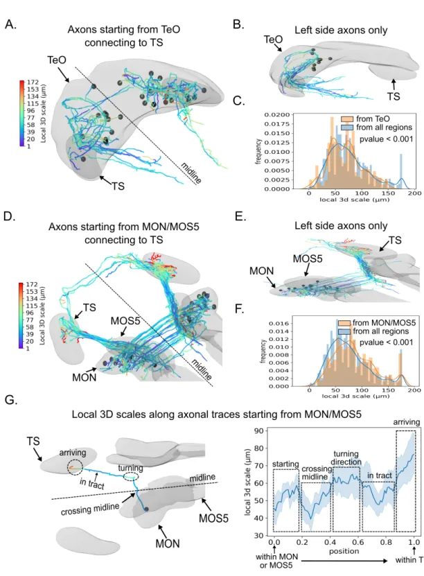
(which was not certified by peer review) is the author/funder, who has granted bioRxiv a license to display the preprint in perpetuity. It is made The copyright holder for this preprint this version posted December 4, 2020.
;
https://doi.org/10.1101/2020.06.01.127035
doi: bioRxiv preprint
To make use of the local dimensionality decomposition across multiple scales and compute a simpler and more intuitive
113
metric, we define the local 3D scale as the highest scale at which the trace still remains 3D. The trace will then locally
114
transform to 2D or 1D for scales higher than that local 3D scale. An example of local 3D scale calculation is shown
115
in Figure 1B. This computation is done at the level of curves; to apply it to whole neuronal arbors, we decompose
116
the arbor into curves by considering, for each ‘leaf’ (terminals), the curves that link it to the root (i.e. the cell body),
117
averaging values when needed (Figure S5). The result is an algorithm that computes a local 3D scale metric for full
118
neuronal arbors, which we term nAdder (see Methods for more details on the algorithm).
119
To test our approach, we examined the local 3D scales of different types of neurons presenting dissimilar arbor shapes,
120
using traces from the NeuroMorpho.Org database (Figure 1C). We first studied a mouse striatal D2-type medium spiny
121
neuron reconstructed byLi et al.(2019) presenting a relatively simple structure with only a few dendrites (Figure
122
1C1, Movie S1). Computation of the local 3D scale for this neuron revealed variations in spatial structure across local
123
regions. For instance, regions (i) and (ii) in Figure 1C1 correspond to two branch segments located at different distances
124
from the soma, and the straightest segment (i) transforms from 3D to 2D and then 1D at a scale smaller than the more
125
tortuous portion (ii). This results in a lower local 3D scale in region (i) (∼40 µm) compared to region (ii) (∼100 µm).
126
We then focused on a mouse cerebellar Purkinje neuron fromChen et al.(2013), presenting a more complex dendritic
127
arbor (Figure 1C2, Movie S2). Most of this arbor was characterized by low local 3D scales (∼45 µm on average), in
128
accordance with the fact that Purkinje cells dendritic arbors have a nearly flat appearance, and hence transform quickly
129
to a 2D plane when scanning the scale space. Nevertheless, the analysis revealed one region (iii) presenting local 3D
130
scales higher than the mean value, which was linked to the fact that dendrites in this region protruded in an unusual
131
manner out of the main plane of the arbor (see Movie S2).
132
Finally, we examined the reconstruction of a mouse retinal ganglion cell (Badea & Nathans,2011) comprising its entire
133
dendritic arbor and the portion of its axon enclosed in the retina (Figure 1C3, Movie S3). We observed small local
134
3D scales (∼35 µm) along most of the axonal trajectory (see region (iv) in 1C3) except in its most proximal portion
135
characterized by high local 3D scales (∼150 µm, region (v)). This reflects the structure of the axon as it first courses
136
in a tortuous manner towards the inner side of the retina before running more directly towards the optic nerve head,
137
the exit point for ganglion cell axons leaving the retina. The proximal region of the axon thus converts from 3D to 2D
138
and 1D much faster than the more distal portion. The dendritic arbor presented an intermediate local 3D scale on the
139
whole (∼80 µm) but with strong local variations. This corresponded to the fact that some dendritic branches exhibited
140
complex shapes whereas others were more direct, as can be seen in Movies S2 and S3.
141
We also compared our local 3D scale metric with two classic local descriptors of 3D traces, curvature and torsion
142
(Figure S6). Mapping of the three parameters in the Purkinje neuron presented in Figure 1C2 showed that the local
143
3D scale provided the most informative measure of the geometric complexity of neuronal arbors, whereas curvature
144
and torsion yielded representations that were difficult to interpret as they were highly discontinuous because of local
145
variations of the curves.
146
Overall, the local 3D scale metric computed with nAdder offers a new local measure of the geometric complexity of
147
neuronal traces, and provides information robust across neuron types, shapes and sizes. We subsequently used our
148
algorithm to reanalyze published datasets in order to explore its capacity to extract biologically meaningful anatomical
149
insights.
150
2.2 Application of nAdder to characterize neuronal arbors during growth and in experimentally altered
151
condition
152
To evaluate the relevance and usefulness of the local 3D scale measure, we first applied nAdder to compare neuronal
153
arbors at different stages of their development and in normal vs. experimentally altered contexts. We selected data from
154
Santos et al.(2018) hosted in the NeuroMorpho.Org database which describe the expansion of the dendritic arbors
nAdder: A scale-space approach for the 3D analysis of neuronal traces
Figure 1: Computation of the 3D local scale of neuronal traces from their multiscale dimensionality decom-position. (A) (left) Variation of the intrinsic dimensionality along a portion of 3D curve; (right) evaluation of the decomposition on simulated trajectories and comparison to a baseline method not based on scale-space (Yang et al.,
2016;Ma et al.,2017). (B) Schematic presentation of the processing of 3D curves by the nAdder algorithm. (C) Application of nAdder to three types of mouse neurons with different arbor shape and size: (C1) striatal D2 medium spiny neuron (Li et al.,2019), (C2) cerebellar Purkinje neuron (Chen et al.,2013), (C3) retinal ganglion cell (Badea & Nathans,2011). The first three columns show the intrinsic dimensionality decompositions of the neurons at small, medium and large scales. The local 3D scale, computed from suites of such decomposition across multiple scales, is shown in the last column. The maximum scale is set at 160 µm based on the longest branch analyzed. Dotted line boxes (i-v) frame areas of interest discussed in the text.
.
CC-BY-NC 4.0 International license
available under a
(which was not certified by peer review) is the author/funder, who has granted bioRxiv a license to display the preprint in perpetuity. It is made The copyright holder for this preprint this version posted December 4, 2020.
;
https://doi.org/10.1101/2020.06.01.127035
doi: bioRxiv preprint
of the Xenopus laevis tectal neuron during development and the effect of altering the expression of Down syndrome
156
cell adhesion molecule (DSCAM). In this study, the authors showed that downregulation of DSCAM in tectal neuron
157
dendritic arbors increases the total dendritic length and number branches, while overexpression of DSCAM lowers
158
them. We reanalyzed neuronal traces generated from the dendritic arbors in this study by computing their local 3D
159
scale using nAdder.
160
Our analysis showed that the mean local 3D scale of developing X. laevis tectal neurons overexpressing DSCAM is
161
smaller than that of control neurons, with a significant difference between the two conditions, 24 and 48 hr after the
162
start of the observations at Stage 45 (Figure 2A and B); this result is consistent with the original analysis bySantos et al. 163
(2018), indicating that DSCAM overexpression leads to more simple arbor morphologies, as measured by the number of
164
branches and length of reconstructed arbors. In their paper, the authors also studied tortuosity, the ratio of curvilinear to
165
Euclidean length of a trace, a global morphological metric classically used to measure geometric complexity. While the
166
authors show that DSCAM downregulation increases the tortuosity of the neuron’s longest dendritic branch (see Figure
167
4 ofSantos et al.(2018)), they did not report this parameter for DSCAM overexpression. We computed the tortuosity of
168
the longest branch and indeed observed no significant difference between control and DSCAM overexpressing neurons
169
at any stage of the analysis (Figure 2C, middle). Interestingly, however, we found that the mean local 3D scale of the
170
arbors’ longest branch (Figure 2C, top) was significant reduced in DSCAM-overexpressing vs. control neurons 24
171
and 48 hr after the start of the image series. We also observed that the length and mean local 3D scale of the neuron’s
172
longest arbor branch were correlated in control neurons (Figure 2D, left) (r = 0.30, p value = 0.020), but disappeared in
173
DSCAM-overexpressing neurons (Figure 2D, right). This suggests a subtle effect of DSCAM in uncoupling the length
174
of neurites and their geometric complexity. Our analysis shows that measuring the neurites’ local 3D scale provides
175
biologically relevant information and can measure subtle differences in the complexity of their trajectory that are not
176
apparent with classic metrics.
177
2.3 Local 3D scale mapping across the whole larval zebrafish brain
178
We next sought to test nAdder over a large-scale 3D dataset encompassing entire long-range axonal projections. A
179
database including 1939 individual neurons traced across larval zebrafish brains and co-registered within a shared
180
framework has been published byKunst et al.(2019). The authors clustered neuronal traces into distinct morphological
181
classes using the NBLAST algorithm (Costa et al.,2016), thus identifying both known neuronal types and putative
182
new ones. These neuronal traces were also used to build a connectivity diagram between 36×2 bilateral symmetric
183
regions identified in the fish brain, revealing different connectivity patterns in the fore-, mid- and hindbrain. Here, we
184
reanalyzed this dataset by computing the local 3D scales of all available neuronal traces, focusing on projections linking
185
distinct brain regions (i.e. that terminated in a region distinct from that of the cell body), interpreted as axons. We then
186
explored the resulting whole-brain map of the geometric complexity of projection neurons.
187
Local 3D scale variations across brain regions. Processing of the 1939 traces of the larval zebrafish atlas with nAdder
188
resulted in a dataset where the local 3D scale of each inter-region projection (i.e. projecting across at least two distinct
189
regions), when superimposed in the same referential, could be visualized (Figure 3A and S7A). Coordinated variations
190
in local 3D scale values among neighboring traces were readily apparent on this map, such as in the retina (see region
191
(i) in Figure 3A) and torus semicircularis (ii) which presented high local 3D scale values, or the octaval ganglion (iii)
192
characterized by low values.
193
To quantify these local differences, we computed the mean local 3D scale of inter region projections for each of the 36
194
brain regions defined by Kunst et al. This enabled us to establish an atlas of the local 3D scale of fish axons highlighting
195
variations of their geometric complexity in different brain regions (Figure 3B and S7B). Similar atlases could be derived
196
for all projection subsets originating from (Figure S8A), passing through (Figure S9A) or terminating in a region (Figure
197
S10A), again showing inter-regional variations. The distributions of local 3D scale within each region nevertheless
198
showed a high variance (Figure 3C, S8B, S9B and S10B), reflecting the diversity of neuronal types and variations in the
nAdder: A scale-space approach for the 3D analysis of neuronal traces
Figure 2: Local 3D scale analysis in tectal neurons from developing Xenopus laevis tadpoles and effect of DSCAM overexpression. Dendritic arbor traces from X. laevis tectal neurons were obtained fromSantos et al.
(2018). (A) Examples of local 3D scale maps from control (left) and DSCAM-overexpressing (DSCAM overexpr) neurons at Stage 45, and 24 and 48 hr after initial imaging. The maximum scale is set to 60 µm based on the mean length of the arbor’s longest branch (highlighted in gray). The cell body’s position is indicated by a black square. (B) Evolution of the mean local 3D scale of the whole dendritic arbor from Stage 45, to +24 and +48 hr. (C) Mean local 3D scale (top), tortuosity (middle) and length (bottom) of the longest branch only. Two-way ANOVA, Student’s t-test with Holm-Sidak for multiple comparisons were used, * p≤0.05, ** p≤0.01, *** p≤0.005, **** p≤0.001. (D) Correlation between the mean 3D scale and the longest branch length in control vs. DSCAM-overexpression conditions. Spearman correlation was used.
.
CC-BY-NC 4.0 International license
available under a
(which was not certified by peer review) is the author/funder, who has granted bioRxiv a license to display the preprint in perpetuity. It is made The copyright holder for this preprint this version posted December 4, 2020.
;
https://doi.org/10.1101/2020.06.01.127035
doi: bioRxiv preprint
local structure of their axons as they exit or enter a brain region. This variability is illustrated in Figure 3D showing
200
three regions, the Medulla Oblongata Strip 3 (MOS3), Subpallium (SP) and Torus semicircularis (TS), respectively
201
presenting low (∼43 µm), medium (∼51 µm) and high (∼58 µm) average local 3D scales. Different patterns exhibited
202
by axons originating from, passing through and arriving in these regions might contribute to this variability (Figure
203
S11).
204
Different distributions of local 3D scale could be observed in the fore-, mid- and hindbrain regions, with higher average
205
value in mid- compared to fore- and hindbrain regions (Figure S7C). The difference is clearer for axons terminating in a
206
region (Figure S10C), but not for axons with soma in these regions and en passant axons (Figures S8C, S9C). This
207
could relate to the observation that the connectivity strength in the mid- and hindbrain are stronger than that in forebrain
208
(Kunst et al.,2019).
209
Comparing the mean local 3D scale with the average number of branching points and average length of the traces within
210
individual regions showed that these parameters were correlated, yet with a high variance (Figure 3E and 3F). However,
211
when separately analyzing axons connecting to, through or from a region, only those originating from the region
212
analyzed showed such correlations (Figures S8D-E), which were not apparent when observing passing or arriving axons
213
(Figures S9D-E and S10D-E). Yet, comparing the local 3D scale of the three types of axons showed that inter-regional
214
axons terminating in a region had on average higher local 3D scales than those originating from or passing through a
215
region (Figure 3G). This observation is consistent with the idea that the proximal axonal path and terminal arbor differ
216
in their complexity, as related to their developmental assembly and function.
217
Together, these results show that the local 3D scale computed with nAdder is informative at the whole brain level,
218
adding a new level of description for analyzing connectomic datasets.
219
Characterization of axon behavior at defined anatomical locations and along specific tracts. A key feature of our
220
metric is its local nature, i.e. its ability to inform on the geometry of single neurites not only globally, but at each
221
point of their trajectory. This aspect is of interest to investigate the complexity of axonal trajectories not simply as
222
function of their origin, but also at specific positions or spatial landmarks. For instance, commissural axons that cross
223
the midline play a major role by interconnecting the two hemispheres and have been well studied, in particular for the
224
specific way by which they are guided across the midline (Chédotal,2014). Examining axonal arbors intersecting the
225
midline in the whole larval fish dataset, we found that a majority (71%) crossed only once, making a one-way link
226
between hemispheres, while a significant proportion crossed multiple times, with 10% traversing the midline more
227
than 5 and up to 24 times (Figure 4A and S12A). Most individual branches (i.e. neuronal arbor segments between two
228
branching points, or between a branching point and the cell body/terminal) crossed the midline just once, meaning that
229
neurons crossing multiple times did not do so with one long meandering axons but with many distinct branches of their
230
arbor (Figure S12B). Examples of such axonal arbors crossing the midline more than 10 times are shown in Figure 4A.
231
Measuring the local 3D scale of crossing axon branches in a 20 µm range centered on the midline (Figure 4B), we
232
observed higher values for the ones traversing the midline several times compared to those only crossing once (Figure
233
4C, top). Axon branches crossing the midline multiple times were also much shorter than those crossing only once
234
(Figure 4C, bottom). They localized mostly in the hindbrain in a ventral position (Figure 4D), while single crossings
235
were frequent in the forebrain commissures. Finally, we found no link between the length and local 3D scale of crossing
236
branches (Figure S12C). This is consistent with the existence of two populations of commissural axons in the vertebrate
237
brain, the hindbrain being home to neurons following complex trajectories across the midline with many short and
238
convoluted branches, and forebrain commissural neurons forming longer and straighter axons.
239
The local 3D scale metric can also serve to compare axon trajectories along entire tracts and characterize their average
240
behavior. To illustrate this, we analyzed two distinct, well known cell types forming long-range axonal projections
241
involved in sensory perception. We used nAdder, first studying the axon trajectories of retinal ganglion cells (RGCs)
242
from the fish atlas, each originating in the retina and terminating in the tectum (Figure 4E). We observed that the
nAdder: A scale-space approach for the 3D analysis of neuronal traces
Figure 3: Local 3D scale mapping across the whole larval zebrafish brain. Traces analyzed correspond to those presented inKunst et al.(2019). (A) Local 3D scale analysis of all axonal traces originating from neurons in the left hemisphere; the maximum scale is set to 100 µm based on the width of the largest brain region. (B) Mean local 3D scales by brain regions. Regions with fewer than 15 traces are excluded (in gray). Values were clipped from the 5th to 95th percentiles for clearer display. (C) Distribution of the local 3D scale values in each brain region (see Table S1 for abbreviation definitions). (D) Examples of local 3D scale mapping for axonal traces in three brain regions respectively presenting low, medium and high mean 3D scale: the Medulla Oblongata Strip 3 (left), the Subpallium (middle), and Torus Semicircularis (right). (E, F) Correlation between the mean local 3D scales and average number of branching points (E) and trace length (F) in different brain regions. Spearman correlation was used. (G) Mean local 3D scale of axons originating from, passing through, and arriving to each brain region. Wilcoxon tests with Holm-Sidak correction for multiple comparison was used, * p≤0.05, ** p≤0.01, *** p≤0.005, **** p≤0.001. Color scale in C, E, F corresponds to that used in B.
.
CC-BY-NC 4.0 International license
available under a
(which was not certified by peer review) is the author/funder, who has granted bioRxiv a license to display the preprint in perpetuity. It is made The copyright holder for this preprint this version posted December 4, 2020.
;
https://doi.org/10.1101/2020.06.01.127035
doi: bioRxiv preprint
local 3D scale of these axons presented clear heterogeneity across regions. To quantify this, we examined RGC axon
244
trajectories in 5 portions of the retinotectal path: within the retina, at the retinal exit, at the midline, just prior to entering
245
the tectum and within the tectum. We observed significant differences between these regions, with the mean local
246
3D scales at the midline presenting low values (∼50 µm) compared to the retina, the tectum, and their exit/entrance
247
regions (∼63 µm). We then used nAdder to analyze a second population, the trajectories of Mitral cell axons originating
248
in the olfactory bulb (OB) and projecting to multiple destinations in the pallium (P), subpallium (SP) or habenula
249
(Hb) (Miyasaka et al.,2014). Here again we found variations in axonal complexity across regions (Figures 4F), with
250
relatively low local 3D scales in the OB (∼40 µm) and Hb formation (∼37 µm) compared to higher values in the P
251
(∼50 µm) and SP (∼47 µm). Overall, this indicates that local 3D scale is a relevant measure of geometric complexity at
252
the single axon level, both to inform on specific points of their trajectory and to compare them within a neuronal class.
253
Local 3D scale analysis of a brain region, the Torus Semicircularis. Finally, we investigated local 3D scale across
254
different axonal populations innervating a given brain region. We performed this analysis in the Torus Semicircularis
255
(TS) which presents a high average local 3D scale, with many complex axonal traces (Figure 3D right panel and S11
256
last row). Most of these traces corresponded to axons with terminations in the TS (70% vs. 5% axons emanating from
257
TS and 25% axons passing through TS). Focusing on this population, we selected three groups of axons originating
258
from the Tectum (TeO), Medial Octavolateral Nucleus (MON) and Medulla Oblongata Stripe 5 (MOS5), respectively,
259
excluding other regions from which only a small number (< 10) of incoming axons had been traced (a detailed list of all
260
regions with traces terminating in the TS is in Table S2). Axons coming from the TeO terminated in the ipsilateral TS
261
(Figures 5A and 5B), in contrast to MON/MOS5 axons which connected the contralateral TS after crossing the midline
262
(Figures 5D and 5E). Examining the distribution of local 3D scale inside the TS, we observed that tectal axons overall
263
had a simpler structure, characterized by lower local 3D scale values than those coming from the MON/MOS5 (Figures
264
5C and 5F). In particular, complex axons with a local 3D scale above 150 µm mostly originated from the MON/MOS5.
265
This difference, revealed by nAdder, points to the existence of divergent developmental mechanisms of pathfinding
266
and/or synaptogenesis for these two populations of axons within a shared target area.
267
We then focused on axons projecting from the MON/MOS5 to the TS. We computed the local 3D scale of these axons
268
at all coordinates of their trajectory from the MON/MOS5 to the TS, normalized with respect to total length (Figure
269
5G). We found that these axons’ local 3D scale was highly correlated and that its average value varied widely along
270
their course from the MON/MOS5 to the TS: low at the start, it increased inside the MON/MOS5 before dropping when
271
the axons crossed the midline. It then increased again as they made a sharp anterior turn, dropped again within the
272
straight tract heading to the TS, before rising to maximum values inside the TS. This result provides a striking example
273
of stereotyped geometrical behavior among individual axons linking distant brain areas, likely originating from a same
274
type of neurons, that our metric is able to pick up and report.
275
Overall, our analysis of the larval zebrafish brain atlas demonstrates that nAdder can be efficiently applied to connectomic
276
datasets to probe structural heterogeneity and identify patterns among individual axons and population of neurons.
277
3
Materials and Methods
278
3.1 Intrinsic dimension decomposition of neurite branches based on scale-space theory
279
Intrinsic dimension decomposition Let’s consider a 3D parametric curve γ(u) = (x(u), y(u), z(u)) for u ∈ [0, 1];
280
the intrinsic dimensionality of that curve can be defined as the smallest dimension in which it can be expressed without
281
significant loss of information. An intrinsic dimension decomposition is a decomposition of a 3D curve into consecutive
282
fragments of different intrinsic dimensionality, i.e. lying intrinsically on a 1D line, 2D plane or in 3D. Note that such
283
decomposition needs not be unique. For example, not taking scales into account, two consecutive lines followed by one
284
plane can in theory be decomposed into one 3D fragment, one 1D and one 3D fragments, two consecutive 1D and one
285
2D fragments, or two consecutive 2D fragments (Figure S1). The last two decomposition schemes are both meaningful
nAdder: A scale-space approach for the 3D analysis of neuronal traces
Figure 4: Local 3D scale analysis of specific locations and axonal tracts of the zebrafish brain. (A) Example of axonal arbors with many branches crossing the midline. (B) Diagram summarizing computation of the local 3D scale at the midline. (C) Local 3D scale (top) and length (bottom) of all axons crossing the midline vs. those crossing only once and more than five times. (D) View of the midline sagittal plane showing the local 3D scale of axons crossing only once and more than five times. The maximum scale is set to 100 µm based on the width of the largest brain region analyzed. (E, F) Local 3D scale variation along axons of retina ganglion cells (E) and mitral cells (F). Wilcoxon tests with Holm-Sidak corrections for multiple comparison were used, * p≤0.05, ** p≤0.01, *** p≤0.005, **** p≤0.001.
.
CC-BY-NC 4.0 International license
available under a
(which was not certified by peer review) is the author/funder, who has granted bioRxiv a license to display the preprint in perpetuity. It is made The copyright holder for this preprint this version posted December 4, 2020.
;
https://doi.org/10.1101/2020.06.01.127035
doi: bioRxiv preprint
Figure 5: Local 3D scale of different axonal populations terminating in the zebrafish Torus Semicircularis (TS). (A, D) nAdder analysis of TS-terminating axons originating from the Tectum (TeO) (A) and Medial Octavolateral Nucleus (MON) or Medulla Oblongata Strip 5 (MOS5) (D). (B, E) Views restricted to axons originating from the left hemisphere. (C, F) Distribution of local 3D scale for the set of axons arriving from the TeO (C) and MON/MOS5 (F) compared to all axons arriving in the TS. Student’s t-test was used. (G) Local 3D scale variations along axons coming from MON/MOS5. Left, example view of one neuron indicating different segments of interest. Right, quantification (n = 32 axons). The maximum scale is set to 175 µm based on the mean length of the longest branches. Only the longest branches are included in the computation.
nAdder: A scale-space approach for the 3D analysis of neuronal traces
and their combination represents a hierarchical decomposition of γ where linear fragments are usually parts of a larger
287
planar fragment.
288
Here, we compute the decomposition of a curve intrinsically by looking at the curvature and torsion. Let us define the curvature κ of γ by κ = kγ0× γ00k/kγ0k3, corresponding to the inverse of the radius of the best approximation of the
curve by a circle locally, the osculating circle. The torsion τ of γ is τ = ((γ0× γ00) · γ000)/kγ0× γ00k2and corresponds
to the rate of change of the plane that includes the osculating circle. We then determine that if κ is identically equal to zero on a fragment then that fragment is a 1D line; similarly τ being identically equal to zero defines a 2D arc curve. Thus we define a linear indicator L of γ:
L(u) = 1, if κ(u) ≤ εκ 0, otherwise, and a planar indicator H of γ:
H(u) = 1, if |τ (u)| ≤ ετ 0, otherwise,
where εκand ετ are the tolerances for computed numerical errors. We note that only using the H indicator is not
289
sufficient to estimate the 2D plane. For example, a 2D plane fragment composed of a 1D line followed by a 2D arc
290
cannot be entirely identified as 2D since the torsion is not defined as the curvature tends to 0. We therefore consider the
291
planar-linear indicator T = L ∪ H instead of H for characterizing the curve according to such hierarchical order.
292
Scale space In practice, the resulting dimension decomposition is closely tied to a ‘scale’ at which the curve is studied,
293
i.e. up-close all diferentiable curves are well approximated by their tangent and thus would be linear. That property
294
have been formalised through Scale-spaces, which have been described for curves in 2D (Mackworth & Mokhtarian,
295
1988) or 3D (Mokhtarian,1988) in particular, to give a robust meaning to that intuition. A scale-space is typically
296
defines as a set of curves γssuch that γ0 = γ and increasing s leads to increasingly simplified curves. The scaled
297
curve can be calculated by convolving γ with a Gaussian kernel of standard deviation s (Witkin,1983), or by using
298
mean curvature flow (Gage & Hamilton,1986). In 2D, it has been shown for example that a closed curve under a mean
299
curvature motion scale space will roundup with increasing s and eventually disappear into a point (Grayson,1987).
300
However, the selection of a scale of interest representing a meaningful description of a curve is not straightforward. A
301
scale defined as the standard deviation of the Gaussian kernel as above for example will be influenced by the kernel
302
length and the curve sampling rate, and would be unintuitive to set. To make the scales become a more relevant
303
physical/biological measurement, we employ as scale parameter the radius of curvature rκ, the inverse of the curvature
304
κ, in µm. For a given curve, the level of detail can be characterized by the maximal rκalong that curve, with scales
305
keeping small rκrepresents high level of detail looking at small objects such as small bumps and tortuosity and scales
306
smoothing the curve out and keeing only larger rκrepresents lower level of detail, and larger object and features such
307
as plateaus or turns. Thus, to ease the interpretation and usage of scale spaces, we associate to a scale in micron ˆrκa set
308
of standard deviation s, by determining, for a curve, for each point u whose rκ(u) < ˆrκthe standard deviation s such
309
that rκs(u) = ˆrκ. This therefore associates, for each curve, an anatomically relevant scale of interest in micron ˆrκand 310
the list S of standard deviations that lead to that curve having no points with curvature radius smaller than ˆrκ. We will
311
then use S to estimate the dimension decomposition of γ at scale ˆrκin two steps, first by computing our indicators for
312
all s ∈ S, then by selecting, across S, the best decomposition.
313
First we compute Lsand Tsby calculating the curvatures κsand the torsions τs. We then exclude fragments smaller
314
than a length threshold εωat every s to eliminate small irrelevant fragments. From Lsand Ts, the linear fragments
315
denoted as DLsand planar-linear fragments denoted as DTsare deduced across all s ∈ S. An example of this sequence 316
of dimension decompositions is illustrated in Figure S4 where DLsand DTs are superimposed. The curve is completely 317
.
CC-BY-NC 4.0 International license
available under a
(which was not certified by peer review) is the author/funder, who has granted bioRxiv a license to display the preprint in perpetuity. It is made The copyright holder for this preprint this version posted December 4, 2020.
;
https://doi.org/10.1101/2020.06.01.127035
doi: bioRxiv preprint
3D at low s value, several linear and planar fragments then appear at higher s, progressively fuse to form larger linear
318
and planar fragments and eventually converge to one unique line at very high value of s.
319
In the second step, we estimate the most durable combination of fragments from the linear segments DLs and linear-320
planar segments DTscalculated in the first step. We compute the number of fragments at every s ∈ S, to measure how 321
long each combination of fragments exists. We then select the combination of fragments remaining for the longest
322
subinterval of S. Knowing that each fragment in the combination can have different lengths among that subinterval, we
323
thus select the longest candidate. In cases where fragments overlap, we split the overlap in half. Of note, we repeat this
324
step twice, first to estimate the best combination of linear-planar segments from DTsinput and mark the corresponding 325
subinterval, then to estimate the best combination of linear fragments from DLsinput within that subinterval. As seen 326
in Figure S4, the curve is decomposed at every s in consecutive planar/nonplanar fragments, then the linear fragments
327
are identified within each planar fragment. The final result is the hierarchical dimension decomposition of the curve γ
328
at a given scale of interest ˆrκ.
329
3.2 Evaluation of dimension decomposition on simulated curve
330
The simulated curve consists of consecutive 1D lines, 2D planes and 3D regions. The simulation of 1D lines is done by simply sampling a sequence of points on an arbitrary axis (e.g. x axis), then rotating it in a random orientation in 3D. The simulation of random yet regular 3D fragments embedded in a 2D plane is more challenging. We tackle this issue by using the active Brownian motion model (Volpe et al.,2014). Active Brownian motion of particles is an extended version of the standard Brownian motion (Uhlenbeck & Ornstein,1930) by adding two coefficients the translational speed to control directed motion and the rotational speed to control the orientation of the particles. At each time point, we generate the new coordinates (x, y, 1) by the following formulas:
DT = kBT 6 π η R DR= kBT 8 π η R3 d dtϕ(t) = Ω + p 2 DRWϕ d dtx(t) = v cos ϕ(t) + p 2 DTWx d dty(t) = v sin ϕ(t) + p 2 DTWy,
where DT and DRare the translational and rotational coefficients, kBthe Boltzmann constant, T the temperature, η
the fluid viscosity, R particle radius, ϕ rotation angle, Ω angular velocity and Wϕ, Wx, Wyindependent white noise.
After generating the simulated intrinsic 2D fragment, a random rotation is applied. For simulating a 3D fragment, we extended the Active Brownian motion model in 2D (Volpe et al.,2014) to 3D as follows:
d dtϕ(t) = cos Ω + p 2 DRWϕ d dtθ(t) = sin Ω + p 2 DRWθ d dtx(t) = v cos θ(t) sin ϕ(t) + p 2 DTWx d
dty(t) = v sin θ(t) sin ϕ(t) + p 2 DTWy d dtz(t) = v cos ϕ(t) + p 2 DTWz,
where (ϕ, θ) are spherical angles. We simulate the curve γ with a sequence of nωconsecutive fragments of varying
331
random intrinsic dimensions. The curve γ is then resampled equally with nγpoints and white noise N (0, σ2) is added.
nAdder: A scale-space approach for the 3D analysis of neuronal traces
We set nω≤ 5, nγ = 1000 points and vary σ between 1 and 30 µm. The upper value of σ = 30 µm is high enough to
333
corrupt local details of a simulated fragment with about 100 µm of length in our experiment.
334
The metric used to measure the accuracy of the intrinsic dimension decomposition, defined to be between 0.0 and 1.0 and measures an average accuracy across fragments, is given by (1/nω)Pimaxjξ(ωi, ˆωj), where {ω1, ω2, . . . , ωnω}
are the simulated intrinsic fragments, {ˆω1, ˆω2, . . . , ˆωnωˆ} the estimated intrinsic fragments and ξ(., .) the F1 score
(Rijsbergen,1979) calculated by:
2 × P recision × Recall P recision + Recall, where P recision = |ω ∪ ˆω| |ω| and Recall = |ω ∪ ˆω| |ˆω| .
In order to evaluate our intrinsic dimensions decomposition algorithm, we look at the curve γ at various scales
335
rκ= 1, 2, . . . , 100 µm, then perform the dimension decomposition for every rκ. Setting rκ= 100 µm is large enough
336
to get a smoothed curve whose simulated intrinsic fragments are no longer preserved. In addition, we also removed
337
estimated fragments whose lengths were smaller than εω. Here we set εω = 5% of the curve length since it does
338
not surpass the minimal length of simulated intrinsic fragments. While automatic determination of an optimal scale
339
is not studied in this paper, with the nAdder algorithm being in part meant to sidestep this complex issue altogether
340
by computing a single metric across scales, we have to chose a scale for the evaluation. We either take the one
341
corresponding to the largest accuracy (optimal scale, Figure S2) or one at a fixed scale (Figure S3), rk= 20 µm, small
342
enough to avoid deforming the simulated curve. Our method is then compared with a baseline method (Yang et al.,
343
2016;Ma et al.,2017) that first iteratively assigns each point on the curve as linear/nonlinear by a collinearity criterion,
344
then characterize nonlinear points as planar/nonplanar by a coplanarity criterion. For both methods, the curve was first
345
denoised based onCzesla et al.(2018).
346
3.3 Local 3D scale computation
347
Assuming a scale interval of interest, the local 3D scale of a point on a curve is computed by iteratively checking at
348
each scale the intrinsic dimension of that point and taking the scale at which the local scale is not 3D anymore. In some
349
cases, the dimension transformation of a point is not smooth, since the point at a 2D/1D scale can convert back to 3D.
350
We therefore select the first scale of the longest 2D/1D subinterval as local 3D scale. In case no subintervals are found,
351
it means that the point remains 3D across the whole interval and its local 3D scale is set as the highest scale.
352
3.4 Local 3D scale analysis of neuronal traces
353
We consider a neuronal trace as a 3D tree and first resample it with a spacing distance between two points equal to 1
354
µm. B-spline interpolation (Boor,1978) of order 2 is used for the resampling. We then decompose the neuronal arbor
355
into potentially overlapping curves, since the intrinsic dimension decomposition and local 3D scale are computed on
356
individual neuronal branches. Several algorithms are available for tree decomposition. We explored three, functioning
357
either by longest branch (first taking the longest branch, then repeating this process for all subtrees extracted along
358
the longest branch), by node (taking each curve between two branching nodes) or by leaf (taking, for each leaf, the
359
curve joining the leaf to the root). Local scales were computed for all three considered decompositions and the ‘leaf’
360
decomposition was found to give the most robust and meaningful results as shown in Figure S5. That method gives
361
partially overlapping curves; thus, we compute the average of the values when needed; we verified that the standard
362
deviations were small.
363
Next, the local 3D scale is computed for each extracted sub-branch within a scale interval of interest. The scale is
364
defined as the radius of curvature and can be selected based on the size of the branches or that of the region studied.
365
For example, in the case of Xeonopus Laevis tadpole neurons (Figure 2), we selected scales from 1 to 60 µm which
366
.
CC-BY-NC 4.0 International license
available under a
(which was not certified by peer review) is the author/funder, who has granted bioRxiv a license to display the preprint in perpetuity. It is made The copyright holder for this preprint this version posted December 4, 2020.
;
https://doi.org/10.1101/2020.06.01.127035
doi: bioRxiv preprint
was sufficient to study neuronal branches of about 180 µm in length (i.e. a 60 µm radius of curvature corresponds to a
367
semicircle with length equal to 60π ≈ 180 µm). In the case of the zebrafish brain dataset (Figure 3), we selected scales
368
from 1 to 100 µm based on the length of the largest region, which was about 300 µm. When studying axons arriving to
369
the Torus Semicircularis (Figure 5), we set the maximum scale to 175 µm as the neuronal branches are on average 525
370
µm long. Moreover, we excluded the sub-branches whose lengths are smaller than a threshold set to 5 µm, which is
371
half the size of the smallest brain region. Branches shorter than 5 µm contribute very little to the local 3D scale result.
372
This is also useful to reduce artifact caused by manual tracing of neurons.
373
3.5 Toolset for neuronal traces manipulation
374
We provide an open source Python toolset for seamless handling of 3D neuronal traces data. It supports reading from
375
standard formats (swc, csv, etc), visualizing, resampling, denoising, extracting sub-branches, calculating basic features
376
(branches, lengths, orientations, curvatures, torsions, Strahler order (Horton,1945), etc), computing the proposed
377
intrinsic dimension decompositions and the local 3D scales. The toolset is part of the open source Python library
378
GeNePy3D (Phan & Chessel,2020) available at https://genepy3d.gitlab.io/ which gives full access to manipulation and
379
interaction of various kinds of geometrical 3D objects (trees, curves, point cloud, surfaces).
380
3.6 Analyzed neuronal traces datasets
381
The traces used in our studies are all open and available online for downloading. They consist of neuronal reconstructions
382
from NeuroMorpho.Org and the Max Planck Zebrafish Brain Atlas listed in the table below:
383
Name Source article Donwload page Search key Note
Medium spiny neuron
(Li et al.,2019) http://neuromorpho.org by neuron name: 3817_CPi_PHAL_ Z001_app2_split_34
Section 2.1
Purkinje neuron (Chen et al.,2013) http://neuromorpho.org by neuron name: Purkinje-slice-age P43-6 Section 2.1 Retina ganglion cell
(Badea & Nathans,
2011)
http://neuromorpho.org by neuron name:
Badea2011Fig2Ca-R
Section 2.1 Xenopus laevis (Santos et al.,2018) http://neuromorpho.org by archive:
Cohen-Cory
Section 2.2 Zebrafish atlas (Kunst et al.,2019) https://fishatlas.neuro
.mpg.de/neurons/download by neuron groups: Kunst et al Section 2.3 384
4
Discussion
385We presented a novel method for the multiscale estimation of intrinsic dimensions along an open 3D curve and used it
386
to compute a local 3D scale, which we propose as a new local metric to characterize the geometrical complexity of
387
neuronal arbors. We demonstrated that our method, dubbed nAdder, is accurate and robust, and applied it to published
388
trace data, showing its relevance and usefulness to compare neurite trajectories from the level of single neurons to the
389
whole brain.
390
Our new approach provides a solution to the problem of measuring the geometrical complexity of 3D curves not just
391
globally but also locally, i.e. at successive points of their trajectory. It enables to compute the dimensionality of such
392
curves at any position, for a given scale of analysis. By scanning the scale space, one can then determine the value at
393
which the curve requires all three dimensions of space for its description, a sampling-independent local metric which
nAdder: A scale-space approach for the 3D analysis of neuronal traces
we term the local 3D scale. Mathematically, scale spaces of curves are trickier to implement in 3D than in 2D and have
395
been much less studied. In 2D for example, scale spaces based on curvature motion are known to have advantageous
396
properties compared to Gaussian ones: they arise naturally from principled axiomatic approaches, are well described
397
mathematically and can be computed through well characterized numerical solutions of partial differential equations
398
(Cao,2003). They are readily extended to 3D surfaces by using principal curvatures (Brakke,2015), but no simple
399
equivalent is known for 3D curves. One theoretical issue is that using only the curvature to determine the motion of 3D
400
curves would not affect the torsion, and for example a set of increasingly tighter helices would have increasingly higher
401
curvature but identical torsion. Here, we provided and thoroughly evaluated a practical solution to this problem by
402
associating a spatial scale to an ensemble of Gaussian kernels. In future work, additional theoretical studies of 3D scale
403
spaces of curves could potentially lead to simpler and more robust algorithms with solid mathematical foundations.
404
The nAdder approach fills a gap in the methodologies available to analyze neuronal traces, which until now were
405
lacking a straightforward way to measure their geometrical complexity and its variations, both within and between
406
traces. It is complementary to techniques classically used to study the topology of dendritic and axonal arbors (number
407
and position of branching points, for example), providing a geometrical dimension to the analysis that is a both simpler
408
and more robust than the alternative direct computation of curvature and torsion. In practice, the local 3D scale of
409
neurons (as measured with nAdder and observed in this study) ranges from 0 to 100-200 µm. The lowest values are
410
typically found in axonal tracts that follow straight trajectories, or in special cases such as the planar dendritic arbor of
411
cerebellar Purkinje neurons shown in Figure 1C2. Higher, intermediate values are for instance observed at inflexion
412
points along tracts where axons change course in a concerted manner. The highest values of local 3D scale typically
413
characterize axonal arbor portions where their branches adopt a more exploratory behavior, in particular in their most
414
distal segments where synapses form. A striking example is given in Figure 5G, showing the trajectory of an axon
415
from the MON/MOS5 to the torus semicircularis, where changes in local 3D scale correlate with distinct successive
416
patterns: a straight section through the midline, a sharp turn followed by another straight section before more complex
417
patterns in the target nucleus. Importantly, nAdder not only enables to quantify how geometric complexity varies along
418
a single axon trace, but also to compare co-registered axons of a same type and to characterize coordinated changes
419
in their behavior (Figure 5G, right panel). It thus offers a way to identify key points and stereotyped patterns along
420
traces. This will be of help to study and hypothesize on the developmental processes at the origin of these patterns, such
421
as guidance by attractive or repulsive molecules (Lowery & Van Vactor,2009), mechanical cues (Gangatharan et al.,
422
2018), or pruning (Lichtman & Colman,2000;Riccomagno & Kolodkin,2015).
423
The high values of local 3D scale near-systematically observed in the most distal part of axonal arbors are also of strong
424
interest, as these segments typically undergo significant activity-based remodeling accompanied by branch elimination
425
during postnatal development (Lichtman & Colman,2000), resulting in complex, convoluted trajectories in adults
426
(Keller-Peck et al.,2001;Lu et al.,2009). In accordance with this, we observed a correlation between local 3D scale
427
and axon branching at the whole brain level (Figure 3E). Further integrating topological and geometrical analysis and
428
linking these two aspects with synapse position could then be a very beneficial, if challenging, extension of nAdder. To
429
this aim, one would greatly benefit from methods enabling both faithful multiplexed axon tracing over long distances
430
and mapping of the synaptic contacts that they establish. Progress in volume electron (Motta et al.,2019), optical
431
(Abdeladim et al.,2019) or X-ray holographic microscopy (Kuan et al.,2020) will be key to achieve this in vertebrate
432
models.
433
Beyond neuroscience, we also expect nAdder to find applications in analyzing microscopy data in other biological
434
fields wherever 3D curves are obtained. For example, it could help characterizing the behavior of migrating cells during
435
embryogenesis (Faure et al.,2016), or be used beside precise biophysical models to interpret traces from single-particle
436
tracking experiments (Shen et al.,2017).
437
Importantly, an implementation of the proposed algorithms, along with all codes to reproduce the figures, is openly
438
available, making it a potential immediate addition to computational neuroanatomy studies. Specifically, nAdder is part
439
.
CC-BY-NC 4.0 International license
available under a
(which was not certified by peer review) is the author/funder, who has granted bioRxiv a license to display the preprint in perpetuity. It is made The copyright holder for this preprint this version posted December 4, 2020.
;
https://doi.org/10.1101/2020.06.01.127035
doi: bioRxiv preprint
of GeNePy3D, a larger quantitative geometry Python package providing access to a range of methods for geometrical
440
data management and analysis. More generally, it demonstrates the interest of geometrical mathematical theories
441
such as spatial statistics, computational geometry or scale-space for providing some of the theoretical concepts and
442
computational algorithms needed to transform advanced microscopy images into neurobiological understanding.
443
Acknowledgments
444This work was supported by Agence Nationale de la Recherche (contract ANR-11-EQPX-0029 Morphoscope2) as well
445
as Fondation pour la Recherche Médicale (DBI20141231328) and Agence Nationale de la Recherche under contracts
446
LabEx LIFESENSES (ANR-10-LABX-65) and IHU FOReSIGHT (ANR-18-IAHU-01).
447
References
448Abdeladim, L., Matho, K. S., Clavreul, S., Mahou, P., Sintes, J.-M., Solinas, X., . . . Beaurepaire, E. (2019, April).
449
Multicolor multiscale brain imaging with chromatic multiphoton serial microscopy. Nature Communications, 10(1),
450
1–14. doi: 10.1038/s41467-019-09552-9
451
Adkins, R. S., Aldridge, A. I., Allen, S., Ament, S. A., An, X., Armand, E., . . . Zingg, B. (2020). A multimodal cell
452
census and atlas of the mammalian primary motor cortex. bioRxiv. Retrieved fromhttps://www.biorxiv.org/
453
content/early/2020/10/21/2020.10.19.343129 doi: 10.1101/2020.10.19.343129
454
Arshadi, C., Eddison, M., Günther, U., Harrington, K. I. S., & Ferreira, T. A. (2020, July). SNT: A Unifying
455
Toolbox for Quantification of Neuronal Anatomy. bioRxiv, 2020.07.13.179325. Retrieved 2020-08-03, from
456
https://www.biorxiv.org/content/10.1101/2020.07.13.179325v1 doi: 10.1101/2020.07.13.179325
457
Ascoli, G. A. (2006, April). Mobilizing the base of neuroscience data: the case of neuronal morphologies. Nature
458
Reviews. Neuroscience, 7(4), 318–324. doi: 10.1038/nrn1885
459
Ascoli, G. A., Donohue, D. E., & Halavi, M. (2007, August). NeuroMorpho.Org: A Central Resource for Neuronal
460
Morphologies. Journal of Neuroscience, 27(35), 9247–9251. Retrieved 2020-05-20, fromhttps://www.jneurosci
461
.org/content/27/35/9247 (Publisher: Society for Neuroscience Section: Toolbox) doi: 10.1523/JNEUROSCI
462
.2055-07.2007
463
Badea, T. C., & Nathans, J. (2011, January). Morphologies of mouse retinal ganglion cells expressing transcription
464
factors Brn3a, Brn3b, and Brn3c: analysis of wild type and mutant cells using genetically-directed sparse labeling.
465
Vision Research, 51(2), 269–279. doi: 10.1016/j.visres.2010.08.039
466
Bates, A. S., Janssens, J., Jefferis, G. S., & Aerts, S. (2019, June). Neuronal cell types in the fly: single-cell anatomy
467
meets single-cell genomics. Current Opinion in Neurobiology, 56, 125–134. Retrieved 2020-05-21, fromhttp://
468
www.sciencedirect.com/science/article/pii/S095943881830254X doi: 10.1016/j.conb.2018.12.012
469
Bates, A. S., Manton, J. D., Jagannathan, S. R., Costa, M., Schlegel, P., Rohlfing, T., & Jefferis, G. S. (2020, April).
470
The natverse, a versatile toolbox for combining and analysing neuroanatomical data. eLife, 9, e53350. Retrieved
471
2020-05-21, fromhttps://doi.org/10.7554/eLife.53350 (Publisher: eLife Sciences Publications, Ltd) doi:
472
10.7554/eLife.53350
473
Boor, C. d. (1978). A Practical Guide to Splines. New York: Springer-Verlag. Retrieved 2020-05-18, from
474
https://www.springer.com/gp/book/9780387953663 475
Brakke, K. A. (2015). The Motion of a Surface by Its Mean Curvature. Princeton University Press.
476
Cao, F. (2003). Geometric Curve Evolution and Image Processing. Berlin Heidelberg: Springer-Verlag. Retrieved
477
2020-05-20, fromhttps://www.springer.com/gp/book/9783540004028 doi: 10.1007/b10404
478
Chen, X. R., Heck, N., Lohof, A. M., Rochefort, C., Morel, M.-P., Wehrlé, R., . . . Dusart, I. (2013, May). Mature
479
Purkinje Cells Require the Retinoic Acid-Related Orphan Receptor-α (RORα) to Maintain Climbing Fiber
Mono-480
Innervation and Other Adult Characteristics. Journal of Neuroscience, 33(22), 9546–9562. Retrieved 2020-07-30,
481
fromhttps://www.jneurosci.org/content/33/22/9546 doi: 10.1523/JNEUROSCI.2977-12.2013
482
Chédotal, A. (2014, October). Development and plasticity of commissural circuits: from locomotion to brain repair.
483
Trends in Neurosciences, 37(10), 551–562. doi: 10.1016/j.tins.2014.08.009