Cardiovascular parameter estimation using a computational model

Cardiovascular Parameter Estimation using a

Computational Model

by

Zaid Samar

Bachelor of Science in Electrical Engineering

Georgia Institute of Technology, 2002

Submitted to the Department of Electrical Engineering and Computer

Science

in partial fulfillment of the requirements for the degree of

Master of Science in Electrical Engineering and Computer Science

at the

MASSACHUSETTS INSTITUTE OF TECHNOLOGY

May 2005

@

Massachusetts Institute of Technology 2005. All rights reserved.

A u th o r ...

...

Department of FlPetrior1

Pr-Tineering

and Computer Science

May 23, 2005

C ertifi(

...

j

Roger G. Mark

Distinguished Professor of Health Sciences and Technology

Professor of Electrical Engineering

Thesis Supervisor

Certified by

...

George C. Verghese

-ofessor of Electrical Engineering

Thesis Supervisor

C ertified by

...

Thomas Heldt

Accepted by ...

Chairman, Department Committee on Graduate Students

MASSACHUSETTS INSTi E OF TECHNOLOGY

To my parents, Yusuf and Nighat.

Cardiovascular Parameter Estimation using a Computational

Model

by

Zaid Samar

Submitted to the Department of Electrical Engineering and Computer Science on May 23, 2005, in partial fulfillment of the

requirements for the degree of

Master of Science in Electrical Engineering and Computer Science

Abstract

Modern intensive care units are equipped with a wide range of patient monitoring devices, each continuously recording signals produced by the human body. Currently, these signals need to be interpreted by a clinician in order to assess the state of the patient, to formulate physiological hypotheses, and to determine treatment options. With recent technological advances, the volume of relevant patient data acquired in a clinical setting has increased. This increase in sheer volume of data available, and its lack of organization, have rendered the clinical decision-making process inefficient. In some areas, such as hemodynamic moni-toring, there is enough quantitative information available to formulate computational models capable of simulating normal and abnormal human physiology. Computational models tend to synthesize information in one common framework, thereby improving data integration and organization. Through tuning, such models could be used to track patient state auto-matically and to relate properties of the observable data streams directly to the properties of the underlying cardiovascular system.

In our research efforts, we implemented a pulsatile cardiovascular model and attempted to match its output to simulated observable hemodynamic signals in order to estimate car-diovascular parameters. Tracking model parameters in time reveals disease progression, and hence it can be very useful for patient-monitoring purposes. As the observable signals are generally not rich enough to allow for the estimation of all the model parameters, we focused on estimating only a subset of parameters.

Our simulations indicate that observable data at intra-beat timescales can be used to estimate distending blood volume, peripheral resistance, and end-diastolic right compliance to reasonable degrees of accuracy. Furthermore, our simulation results based on a real patient hemorrhage case reveal that clinically significant parameters related to bleeding rate and peripheral resistance can be tracked reasonably well using observable patient data at inter-beat timescales.

Thesis Supervisor: Roger G. Mark

Title: Distinguished Professor of Health Sciences and Technology Professor of Electrical Engineering

Thesis Supervisor: George C. Verghese Title: Professor of Electrical Engineering Thesis Co-Supervisor: Thomas Heldt Title: Postdoctoral Associate

Acknowledgments

I would like to thank Professor Roger Mark and Professor George Verghese for their guidance and support throughout my time at MIT. I am extremely fortunate to have been groomed under both of them, and I am in total awe of the keen insight with which they have guided me.

I would also like to thank Dr. Thomas Heldt who has been a source of inspiration and guidance, not only in matters related to research, but in all aspects of graduate student life in general. I am also grateful to him for his assistance during the writing of this thesis.

I am indebted to Tushar Parlikar and Carlos Renjifo for their support and encouragement throughout. Together, we were the first student members of the 'modeling group' and I have had a great time working with them. From our initial sporadic meetings in TA rooms to our weekly meetings in the LEES headquarters, we have come a long way and it has been a lot of fun.

A special thanks to all the members of the Laboratory of Computational Physiology who made my stay there an endearing one. I would like to thank Mohammed Saeed who introduced me to the group's activities which subsequently captured my interest in this area of research. Mohammed also introduced me to the powerful domain of Simulink. I would like to thank Dr. Gari Clifford for all his help and support. I am also thankful to Gari for driving me to exercise in the form of playing squash with him (before my laziness got the better of me). I would like to thank James Sun, Tin Kyaw and Omar Abdala for their support and friendship. I am especially thankful to James Sun for his contributions towards our work. I am grateful to Dr. Brian Janz and Dr. Andrew Reisner for their expert medical insight which allowed us to move forward with our research goals.

I want to thank Adnan Dosani, whose friendship and support played important roles in my decision to join MIT. Throughout my undergraduate and graduate school experiences, Adnan has always been there to share my grievances and celebrate my moments of success and happiness.

support, prayers, and good wishes. I have known these guys for more than a decade now and I am grateful that we are still very much in touch , despite the distances that separate us.

I thank Rehan Tahir, Zubair Anwar, and Faisal Kashif for their support and culinary skills. Their friendship, and the food which they fed me, have made my MIT experience a memorable one. Faisal also provided me with much needed company at odd hours of the night during the writing process, for which I am grateful. I would also like to thank Hasan Ansari for his friendship and support; his antics have always managed to bring a smile to my face.

Finally, I come to those who matter most. I would like to thank my sister, Maleeha, for her love and support. She has always been the elder sibling who has looked out for me at every stage. I would like to express my deepest gratitude to my parents, Yusuf and Nighat, for all the sacrifices they have made to provide me with the very best. Their love, support, and prayers have been the driving force behind all my achievements.

This work was supported in part through the National Aeronautics and Space Admin-istration (NASA) through the NASA Cooperative Agreement NCC 9-58 with the National Space Biomedical Research Institute and in part by Grant ROl EB001659 from the National Institute of Biomedical Imaging and Bioengineering.

Contents

1 Introduction 17

1.1 M otivation . . . . 17

1.2 The Cardiovascular System . . . . 19

1.3 Cardiovascular Models and Model-Based Reasoning . . . . 20

1.4 Hemodynamic Monitoring in an ICU . . . . 21

1.5 Thesis Goals and Outline . . . . 23

2 The Computational Hemodynamic Model 25 2.1 Simplifying Assumptions . . . . 26

2.2 C V SIM . . . . 26

2.3 The Model Implementation . . . . 28

2.3.1 The Platform . . . . 28

2.3.2 Nominal Parameter Values . . . . 28

2.3.3 The Time-Varying Compliance Function . . . . 29

2.3.4 The Model Dynamics . . . . 30

2.3.5 Initial Conditions . . . . 32

2.3.6 Conservation of Volume . . . . 33

2.3.7 Model Validation . . . . 35

2.3.8 Interstitial Fluid Compartment . . . . 36

3 The Cardiovascular Control System

3.1 Arterial Baroreflex . . . . 3.2 Implementation . . . . 3.2.1 Preprocessing and Error Calculation 3.2.2 Effector Mechanism . . . . 3.3 Qualitative Validation . . . . 3.3.1 Hemorrhage . . . . 3.3.2 Left Myocardial Infarction (MI) . . . 3.4 Concluding Remarks . . . .

4 Parameter Estimation using Waveform Data

4.1 Non-linear Least Squares and Subset Selection . . . . 4.1.1 Non-linear Least Squares Optimization . . . . 4.1.2 Subset Selection . . . . 4.1.3 Jacobian Calculation and Scaling . . . . 4.1.4 Application of the Subset Selection Algorithm . . . . 4.1.5 Description of the Estimation Problem . . . . 4.2 R esults . . . . 4.2.1 Estimation using Steady-State Waveform Data . . . . 4.2.2 Estimation using Transient Waveform Data (Hemorrhage Data) 4.3 Concluding Remarks . . . .

5 Parameter Tracking using Beat-to-Beat Averaged Data

5.1 Brief Patient History . . . . 5.2 Patient Data for Parameter Tracking . . . . 5.3 Simulating Patient Data . . . . 5.4 Parameter Tracking . . . . 5.5 R esults . . . . 5.6 Concluding Remarks . . . . 43 . . . . 44 . . . . 44 . . . . 45 . . . . 46 . . . . 51 . . . . 51 . . . . 52 . . . . 53 55 56 56 58 60 62 63 63 63 66 69 71 72 72 74 77 80 81

6 Conclusions and Recommendations for Future Work 83 6.1 Sum m ary . . . . 83 6.2 Recommendations for Future Work . . . . 85

A Updated CVSIM Model Equations 89

B Independent Parameters of the CVSIM Model 93 C Peripheral Resistance Estimation based on Patient Data 95

C.1 Assumptions on Changes in Peripheral Resistance ... 95 C.2 Peripheral Resistance Estimation using the Windkessel Model . . . . 96 C.3 Concluding Remarks . . . 100

List of Figures

1-1 The Circulation System [1]. . . . . 20 2-1 Circuit analog of the CVSIM model. . . . . 27 2-2 Ventricular compliance function and its derivative. . . . . 30 2-3 Difference between expected total blood volume (Qrotal) and calculated total

blood volume (QTotal), with left and right ventricular pressure (voltage) as

state variables. . . . . 34 2-4 Difference between expected total blood volume (Qrotal) and calculated total

blood volume (QTotal), _{with left and right ventricular volume (charge) as state}

variables. . . . . 34 2-5 Pulsatile pressure waveforms for a single beat. . . . . 36 2-6 Volume distribution for an average 70-kg adult. Approximately 60% of body

mass is fluid. This percentage can vary depending on age, sex, and obesity [2]. 37 2-7 Addition of the interstitial compartment between the systemic arteries and

vein s. . . . . 39 2-8 Beat-to-beat averaged venous charge (Q"V) vs time. Sub-figure (a) shows the

plot of Qav vs time before and after the administration of a fluid bolus. Sub-figure (b) shows the plot of ln(Qav) vs time, and its best straight line fit, after the administration of a fluid bolus. The time-constant for the charge decay is the reciprocal of the slope of the best straight line fit: Tit ~ 4.5 min. . . . . 40

3-1 Block diagram of the arterial baroreflex system. P'f is the set-point pressure that the system is aiming to maintain. . . . . 45 3-2 Block diagram depicting the preprocessing involved. . . . . 46 3-3 Impulse response and magnitude of Fourier transform of sympathetic and

parasympathetic filters. The impulse responses are estimated from canine d ata [3]. . . . .. 47 3-4 Diagrammatic representation of the effector mechanism depicting autonomic

m ediation. . . . . 48 3-5 Open-loop step responses of sympathetic and parasympathetic filters as

im-plemented using Simulink. . . . . 50 3-6 Actual parasympathetic impulse response and its Pad6 approximations. . . . 51 3-7 Open-loop step response comparison of the parasympathetic filter and its

approxim ations. . . . . 52 3-8 Parasympathetic block output during hemorrhage and left MI simulations

using different approximations for the parasympathetic filter. . . . . 53 3-9 Hemorrhage simulation. . . . . 54 3-10 Left M I sim ulation. . . . . 54 4-1 Eigenvalue spectrum of the Hessian approximation under the two different

scaling schem es applied. . . . . 62 4-2 Estimated active parameters recovered using steady-state waveform data vs

actual active parameters. . . . . 65 4-3 Estimated vs actual change in DBV for all the simulated hemorrhage cases

analyzed . . . . . 67 4-4 Estimated vs actual Ra for all the hemorrhage cases analyzed. . . . . 68 4-5 Estimated Cd vs actual Ced for the hemorrhage cases. . . . . 69 5-1 Heart rate (upper panel) and arterial blood pressure (lower panel) patient data. 73 5-2 Levophed administration (top panel) and beat-to-beat averaged patient ABP

5-3 Simulated beat-to-beat averaged ABP data (top panel) and actual patient ABP data (bottom panel). . . . . 76 5-4 Beat-to-beat averaged ABP data: actual and simulated with additive noise. 77 5-5 Simulated beat-to-beat averaged CVP data. . . . . 79 5-6 Diagram depicting the neglect of intra-beat dynamics under the proposed

scheme to estimate initial conditions. . . . . 80 5-7 Plot showing portion of ABP data following a fluid bolus and its reconstructed

version using exact parameters and estimated initial conditions using two different schem es. . . . . 81 5-8 Estimated versus actual parameters. . . . . 82 A-i Circuit analog of the updated CVSIM model. . . . . 90 C-1 Beat-to-beat averaged patient ABP data (top panel) and Levophed medication

(bottom panel). . . . . 96 C-2 Circuit analog of Windkessel model. Pa refers to arterial blood pressure. . . 97 C-3 Windkessel estimate of Ra (top panel), beat-to-beat averaged patient ABP

data (middle panel), and Levophed medication (bottom panel). . . . . 98 C-4 Windkessel estimate of Ra incorporating the non-linearity in Ca (top panel),

beat-to-beat averaged patient ABP data (middle panel) and Levophed med-ication (bottom panel). . . . . 99

List of Tables

2.1 Nominal parameter values for the CVSIM model. . . . . 29 2.2 Comparison between model outputs and reported norms for compartmental

pressures, stroke volume and cardiac output. . . . . 35 3.1 Nominal parameter values for the arterial baroreflex model. The values are

taken from Davis's implementation [4]. . . . . 49 4.1 Parameters identified as being well-conditioned by the subset selection

algo-rith m . . . . . 62 4.2 Estimation error statistics for the active parameters under two schemes:

esti-mating only the active parameters with the ill-conditioned ones fixed at their nominal values, and estimating all the model parameters. . . . . 64 4.3 Estimation error statistics for the active parameters with C, and Cfd fixed at

their actual values. . . . . 66 B.1 Independent Parameters of the CVSIM Model (adapted from Heldt [5]). . . . 94

Chapter 1

Introduction

1.1

Motivation

Patient care for the critically ill is provided in dedicated hospital departments known as Intensive Care Units, or ICUs. Patients suffering from various conditions, such as unstable

cardiovascular disease, multiple-organ failure, or severe trauma, are usually admitted to the ICU. Though the reasons behind admissions are varied, ICU patients have one thing in common -they are often in a fragile condition which requires close monitoring of the state of the patient to guide the course of treatment, or to allow for rapid intervention if the patient's state deteriorates.

To help accomplish this, modern ICUs are equipped with a wide range of monitoring equipment, each continuously recording a series of physiological signals. These detailed measurements are supplemented with frequent laboratory tests and imaging studies from different hospital departments. The logistics involved in data collection from different de-partments and the high volume of data, coupled with poor data integration and organization, complicate and prolong the clinician's task of formulating physiological hypotheses and de-termining treatment options. However, timely and accurate patient care is of utmost impor-tance in an ICU setting where patients require immediate and often proactive action. Thus, the increase in sheer volume of data available, and its lack of organization, have rendered the

clinical decision-making process inefficient. Presenting all the available information without regard to relevance can often lead to oversight of important factors which can cause serious, possibly fatal, errors in an ICU setting. This phenomenon is generally known as the problem of information overload which has contributed to several historical catastrophes including the New York City blackout of 1977 [6].

In addition to the information overload problem, ICUs suffer from inaccurate alarm systems. Bedside alarms sound an alert whenever an individual measured signal exceeds or drops below some predefined value, an event that occurs quite often with no physiological basis, as for example, when excessive patient movement interferes with electrode contacts and position. Individual signals being monitored are usually correlated and interdependent. However, current representation of these signals does not incorporate these relationships, which results in too sensitive an alarm system. In fact, several studies have shown that over 80% of these single-variable alarms are false positives [7], leading to misallocated resources and desensitization to alarms.

The inability of the ICU monitoring systems to evaluate the state of the patient efficiently increases the chances of human error. Donchin et al. [8] conducted a study in which they estimated that 1.7 human errors occur per patient per day in the ICU they observed. One of the reasons for the errors was attributed to difficulties in assessing patient state, a function which is directly affected by the limitations of the current monitoring systems coupled with the information overload problem.

The problems encountered in ICU patient monitoring motivate the use of computational models. Representing a physiological system in a mathematical form aids in understanding how the various components interact with each other to influence the outputs. Computa-tional models tend to synthesize information in one common, holistic framework thereby improving data integration and organization. Given current computational power, compu-tational models can cycle through many iterations of hypothesis-generation and test their compatibility with experimental data. Furthermore, computers tend to be more vigilant than humans. Thus, computational models might be able to learn from clinical data and

help significantly in developing physiological hypotheses regarding a patient's state.

The cardiovascular system is an area which has been subjected to various modeling studies (see Section 1.3). There is enough knowledge about the cardiovascular system to formulate mathematical models that describe all the inter-component relationships accurately. Such models may be useful in helping to assess patient state, and if so, they can be employed to aid in patient monitoring.

1.2

The Cardiovascular System

The human cardiovascular system is responsible for circulating blood throughout the body to perfuse the tissues with nutrients and oxygen, and remove the waste products. The system includes the heart muscle, which acts as a pump, and the blood vessels through which the blood flows (see Figure 1-1).

There are three main kinds of blood vessels: arteries, veins and capillaries. The arteries carry blood from the heart to the tissues at high pressures. As blood is transported to the rest of the body, arteries branch out into smaller vessels through which blood is transported to individual organs. Within the organs, the exchange of oxygen and nutrients takes place through the walls of thin vessels known as capillaries. The veins, which constitute the low pressure carrying component of the system, transport blood back to the heart.

The heart consists of four chambers -two atria (left and right), each of which is connected to a ventricle. The pumping action of the heart is quasi-periodic in nature, the rhythm of which is governed by electrical impulses generated by the sino-atrial node. A cardiac cycle consists of two regimes of operation: diastole and systole. During the period of diastole, the ventricles are relaxed and fill with blood, whereas in systole, the ventricles contract and eject blood into the circulation. The left ventricle pumps oxygenated blood to the rest of the body (systemic circulation). After the exchange of nutrients and oxygen, de-oxygenated blood is returned to the right ventricle which then pumps the blood through the lungs (pulmonary circulation) where gaseous exchange occurs. The newly oxygenated blood is then driven into the left ventricle from whence the cycle continues.

02

Figure 1-1: The Circulation System [1].

As the cardiovascular system maintains blood flow, a model that accurately represents this system can be used to gain insight into the hemodynamic changes occurring in patients.

1.3

Cardiovascular Models and Model-Based

Reason-ing

An analogy exists between computational models of cardiovascular function and electrical circuits, a parallel that has been exploited since the late 1800's. Moens and Korteweg used

transmission-line theory to describe quantitatively the circulation system in 1878. Around twenty years later, Frank introduced the Windkessel model, which consisted of a simple

first-order circuit to model arterial dynamics [9]. With the advent and widespread use

of digital computing, a wealth of research has been directed towards the development of computational cardiovascular models that adequately represent the underlying physiology and hemodynamics. The models vary in degree of complexity, with the 'Guyton Model',

consisting of the combined physiological insight of Dr. Guyton and his associates, being the most comprehensive

[10].

The purpose behind model development is to gain insight into physiological phenomena within a closed framework. Much of the mentioned modeling work has been directed towards forward-modeling, which consists of tweaking model parameters so that the system can output realistic data that match observations. Recently, however, interest has been generated in inverse-modeling, or parameter estimation, where the system parameters are estimated on the basis of observed data. Various techniques, including gradient-based error minimization using underlying computational models, have been used to estimate cardiac function [11], and arterial parameters [11, 12, 13].

Cardiovascular parameter estimation can provide an integrated structure that can be used to asses the patient's hemodynamic state. Knowledge of the changes in specific para-meter values can help monitor patient trajectory and guide clinical interventions. Motivated by the advantages of model-based estimation and reasoning, Zhao developed a set of heuris-tic algorithms to estimate 7 of the 17 independent parameters in the underlying lumped parameter, 6-compartment, cardiovascular model [14]. The system evaluated the parame-ters by iteratively matching the model output to pseudo-patient data. This was achieved by tweaking the model parameters based on some underlying logic using artificial intelligence. The algorithms were tested on steady-state, static, simulated data and were found to per-form reasonably. However, such a system cannot be used for continuous monitoring as the algorithms use certain measurements that are only intermittently available, for example, left ventricular end-diastolic pressure (LVEDP). Moreover, the steady-state assumption is not always valid in unstable patients. In order to help monitor patients continuously, the esti-mation algorithm has to be devoid of the steady-state assumption and it has to be limited to using what is constantly measurable in an ICU.

1.4

Hemodynamic Monitoring in an ICU

" Electrocardiograph (ECG): ECG is a recording of the body surface potentials generated by the electrical activity of the heart. ECG recordings are important indicators of the state of the heart and are extensively used for diagnosis of cardiac conduction abnormalities (arrhythmias), ischemia, infarction, hypertrophy, etc. Moreover, ECG monitors record heart rate (HR) and rhythm which are important factors in judging the stability of all patients.

" Systemic Arterial Blood Pressure (ABP): ABP is monitored invasively using an arterial line inserted into an accessible artery. The preferred site of insertion is the radial artery on the wrist as it is easily accessible and simple to keep clean. Continuous ABP monitoring is essential as abnormal ABP is indicative of diseased states. In addition, continuous ABP monitoring serves as a feedback to clinical interventions such as medication. The monitoring system records ABP waveforms and also computes derivable quantities such as systolic, diastolic, and mean pressures.

" Central Venous Pressure (CVP): CVP waveforms are monitored by inserting a venous catheter into a peripheral vein and by advancing the catheter through the subclavian vein and the superior vena cava. CVP is an important determinant of right ventricular function as it correlates with the filling pressure of the right heart.

" Pulmonary Artery Pressure (PAP): The introduction of PAP monitoring has been one of the most popular and important advances in patient monitoring [15]. Although recently PAP recordings have become subjected to increased scrutiny, it is not uncom-mon to have patients inserted with a Swan-Ganz catheter to record PAP waveforms. The catheter is inserted into a peripheral vein, and it is pushed past the right atrium and ventricle until it enters the pulmonary artery. The tip of the catheter is fitted with a balloon, which, when inflated, obstructs flow and gives a measure of left ventricular filling pressure.

" Cardiac output (CO) is an important hemodynamic parameter which can be measured intermittently in an ICU. CO is a measure of the blood volume pumped by the heart

per minute and hence it is an important indicator of cardiac function. CO is usually measured by the thermodilution technique in which a patient is administered a bolus of cold liquid. The ensuing temperature changes, measured by a thermistor attached to a catheter, are then plotted over time forming what is known as the thermodilution curve. A measure of CO is obtained by exploiting its inverse relationship to the area under the thermodilution curve.

1.5

Thesis Goals and Outline

In this thesis, we explore model-based quantitative methods for estimating selected cardio-vascular parameters over time. Tracking the time evolution of these parameters would not only aid in determining patient state, but it may also help in identifying the onset of com-plications, thereby increasing the quality and effectiveness of patient care. The data used for estimation is limited to what can be monitored continuously in an ICU. This includes waveforms and other derivable quantities of ECG, ABP, CVP, and PAP. The challenge lies in using a small number of observable signals to perform parameter estimation based on an underlying high-detail model. To overcome this difficulty, we focus on estimating only a subset of parameters.

In chapters 2 and 3, we detail the computational cardiovascular model used for our investigation and we describe its implementation in Simulink.

In chapter 4, we use synthetic waveform data to estimate cardiovascular parameters using a non-linear least squares optimization technique along with subset selection - an algorithm that identifies a subset of parameters that can be estimated robustly.

In chapter 5, we explore a real hemorrhage case. We attempt to track the bleeding rate and the rate of change of peripheral resistance using beat-to-beat averaged data. Accurate knowledge of the value of these two parameters is critical in treating any hemorrhage case.

Chapter 2

The Computational Hemodynamic

Model

A strong analogy exists between electric circuits and fluid systems. Computational models of the cardiovascular system are therefore conveniently represented in the form of their circuit analogs. The vessels can be thought of as capacitors with compliances (C, m"7r ) that store

blood volume

(Q,

mL), connected to resistors (R, mLHs or PRU) which account for the fluid resistance faced by blood flow. The ventricles can be modeled as capacitors with time varying compliances. During diastole, ventricular compliance is high which allows the ventricles to store blood volume, thus mimicking the act of being filled. During systole, however, ventricular compliance decreases, thus increasing pressure, which leads to the emptying of the chamber. A periodic compliance function which varies between the diastolic and systolic compliance values can therefore be used to model the pumping action of the heart. Using this circuit analogy, blood volume maps to charge, blood flow rate

(4,

mL/s) to current, and

pressure (P, mmHg) to voltage. In this chapter, we describe the cardiovascular model used

2.1

Simplifying Assumptions

It would be practically impossible to construct a model with a manageable level of complexity, that accounts for all the nuances of cardiovascular function. A great simplifying assumption in this regard is that the cardiovascular system can be represented by a lumped parameter model. Dispersed networks, such as that of the arteries and arterioles, can therefore be modeled using single circuit elements. Lumping the parameters together reduces the ability of the model to represent distributed behavior, such as pulse reflections, however, such level of detail is currently not the focus of our investigation.

Another simplifying assumption is that the circuit elements are linear. For the capacitors, this assumption is reasonable over the range of pressures for which the elastic fibers of the vessels are stressed, leading to an approximately linear volume-pressure relationship. Beyond this range, collagen fibers become stressed and add an element of non-linearity. The systemic arteries, however, exhibit non-linear compliance over all pressure ranges due to the presence of multiple tensions. Moreover, the pulmonary arterial resistance is notably non-linear in behavior as well

[16].

However, for the sake of simplicity, these elements can be considered as linear without compromising appreciably the ability of the model to represent the cardiovascular system for the purposes of our investigation.

2.2

CVSIM

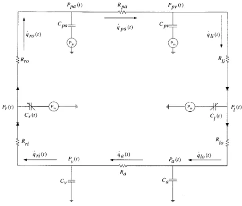
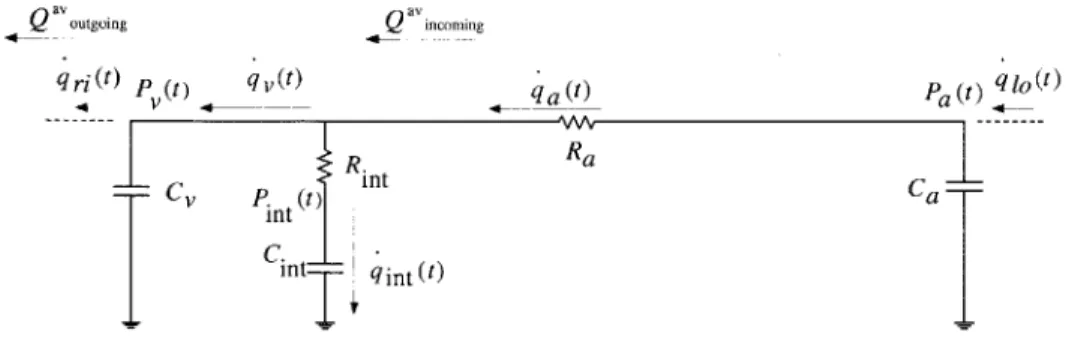
The Cardiovascular Simulator, or CVSIM, was originally developed by Davis as an aid in teaching cardiovascular physiology [4]. Figure 2-1 shows the model in its circuit represen-tation. CVSIM comprises six compartments which model the left and right ventricles (1, r), the systemic arteries and veins (a, v), and the pulmonary arteries and veins (pa, pv). The atria are excluded from the model because they play no significant hemodynamic role during normal heart rates. During increased heart rates, as may be the case in disease conditions, atrial contraction may contribute significantly to stroke volume. However, the effects of the atria can be accounted for by modifying the right ventricular parameters [4].

Pr(t) Cr(t) ri ri(t) _P (t)

~pa

(t)RAA Ra Cv

Figure 2-1: Circuit analog of the CVSIM model.

The ventricles are modeled by time-varying compliances connected to inflow and outflow resistances (R(l,r)i, R(1,r)o) that represent resistance encountered by blood flow as it enters and exits the ventricles. The time-varying compliance is completely characterized by the beat period (T), and by its minimum (end-systolic (es)) and maximum (end-diastolic (ed)) values (see Section 2.3.3). The rest of the compartments are each modeled by a linear capacitor coupled with a linear resistor. The resistances for the systemic and pulmonary veins are lumped with the right and left ventricular inflow resistances respectively. Each capacitor acts as a storage for blood volume as determined by the characteristic relationship:

(2.1)

where the subscript i refers to any of the six compartments.

Qj

is referred to as the stressed

q pa W qro(t ) Rro C| W R1 Pa) W q 1 (t) P(t) Ca-Ppa (t) Rpa Ppv (t ) Cpa--Pt q i;) R q at)

Qi = Ci _ (p

i _ p

rel)

compartment volume. To represent the volume of the compartment at zero-pressure, each compartment has another volume parameter,

Q0,

associated with it. The reference pressure,

Pfi, is ground for the systemic circulation and intrathoracic pressure (Pth) for the rest of the compartments as they reside inside the thorax. Although Pth is known to vary with respiration, it can be modeled reasonably well as a constant equal to its average value. The diodes constitute the only non-linear elements of the model and act as cardiac valves that ensure uni-directional blood flow through the ventricles.

We chose to use the CVSIM model because of its reasonable level of complexity and its remarkable ability to model normal cardiovascular dynamics. Moreover, it was also previ-ously used successfully to model some steady-state disease conditions, thus demonstrating its ability to model abnormal conditions as well [4, 14].

2.3

The Model Implementation

2.3.1

The Platform

We developed the model in Simulink 1 which is a strong tool for implementing dynamic systems. Simulink allows for a good degree of abstraction by providing building blocks with built-in functions and routines. The model becomes easily extendible which is advantageous for simulating various disease conditions. Another advantage of this platform is the fact that it is automatically interfaced with Matlab which makes the analysis and presentation of data very convenient.

2.3.2 Nominal Parameter Values

The nominal parameter values were determined by Davis for a 70-kg individual

[4].

We use his values which are summarized in Table 2.1.

Table 2.1: Nominal parameter values for the CVSIM model.

Compartment c, m Q, rmL R, "m"ig-s (PRU)

left ventricle (1) 0.4 - 10 15 0.006 (Rio -left ventricular outflow resistance)

systemic arteries (a) 1.6 715 1.0

systemic veins (v) 100.0 2500 0.01 (Ri - right ventricular inflow resistance) right ventricle (r) 1.2 - 10 15 0.003 (Rro - right ventricular outflow resistance) pulmonary arteries (pa) 4.3 90 0.08

pulmonary veins (pv) 8.4 490 0.01 (Ri - left ventricular inflow resistance)

System parameters: T = 5 s

Pth = -4 mmHg

Qtotal = 5000 mL

2.3.3

The Time-Varying Compliance Function

The compliances of the ventricles are based on the ventriclular model of Suga and Sagawa [17, 18]. The time evolution of the compliance function is given below, as outlined by Mukkamala

[16],

in the form of its inverse, called elastance (E).

1( 1 Ei,r(t)

I

, 1l~ ced _r ( COS(,(tti))) +_Tl r - J . ( + COS(2,(t iT))) + C I'r TS1.r ti < t < tj + Ts ti + TS < t < ti + Ts + Tir ti + T + Tir ; t < ti+1

where the subscript i refers to the ith cardiac cycle. T, and Ti, refer to the systolic time period and the time for isovolumetric relaxation, respectively. These two parameters are related in the following manner:

(2.3)

(2.4)

T5 0.3V T

Ti -2

-2 2

The time period for diastole, Td, can therefore be calculated as follows:

Td = T - Ts - T, = T - 0.45vIT (2.5)

(2.2)

C(t) Cr(t) 10 8-6 4 2 01 0 0.1 0.2 0.3 0.4 0.5 0.6 0.7 0.8 0.9 time in s

(a) Compliance function over one cardiac cycle.

Aflfl 200 -0 00 0 1 0.2 0.3 0.4 0.5 0.6 0.7 0.8 0.9 dC2 1E0 - 0-0 0-0.1 0.2 0.3 0.4 0.5 0.6 0.7 0.8 0.9 01U0 0.1 0.2 0.3 0.4 0.5 0.6 0.7 0.8 0.9 time in s

(b) Derivative of the compliance function over one cardiac cycle.

Figure 2-2: Ventricular compliance function and its derivative.

Figure 2-2a shows the compliance function over one cardiac cycle.

2.3.4

The Model Dynamics

Applying Kirchoff's Current Law (KCL) to the circuit topology of the model, the following set of equations is obtained:

dP dt dPa dt dPv dt dPr dt dPpa dt dP v dt

41i - 41o - (P1 - Pth)

-dCi(t)/dt

C₁(t) _41o - 4a Ca _4a - 4ri 4ri - ro- (Pr - Pth)

-

dCr(t)/dt

Cr(t) _ ro - qpa Cpa _ a - 4ii ~CPV (2.6) (2.7) (2.8) (2.9) (2.10) (2.11) 10 _ 6 4 -2 2 0-0 0.1 0.2 0.3 0.4 0.5 0.6 0.7 0.8 0.9 I

The compartmental flow rates are obtained through the application of Ohm's Law: P ,if P", > P dlj = (2.12)

0

otherwise PI-P i f Pi>Pa 410 = P , (2.13)

0

otherwise P-P qa = Pa Pv (2.14) Ra P ,i f

PV

> Pr 4,i = Rj(2.15) 0 otherwise PP->Ppa 4ro = "r fP p (2.16) 0 otherwise Pa = Ppa - Pp (2.17) Rpv

Equations 2.6 - 2.11 give the time derivatives of the compartmental pressures, which act as state variables. The system of equations can be solved by discretizing the problem. Given an initial set of pressures, the corresponding flow rates are calculated which are used to determine the local gradient information for the pressures. The pressure gradients are then integrated over time to obtain the compartmental pressures at the next time step. Once the new set of pressures is obtained, the cycle continues and the system is evolved iteratively in time. The integration routine used is the standard, fourth-order Runge-Kutta method with a fixed step-size of 0.005 s [19]. The fixed step-size is on the order of the smallest time-constant of the system and it is smaller than 0.006 s, which was identified as the maximum allowable step-size by Davis [4]. The details of the model implementation outlined here, including the choice of state variables, are similar to previous realizations of CVSIM [4, 16].

2.3.5

Initial Conditions

The initial conditions for the state variables are obtained by employing the method used by Davis

[4].

A set of linear equations, formulated on the basis of conservation of volume (charge), are solved to obtain the end-diastolic pressures which are used as initial conditions for the start of a cardiac cycle.

Cd(Pi"e - Pt h) -

C"

(P - Pt h) Qtotal - Qtotal - C~d( P~d - Pth) - CS(Ps - Pth)

TSP,

_ - Pa R10 =T Pa - v Ra p - ped - Td " R1 r = TSe , - pa Rro T pa - Ppv Rpa P -P led Rij = Cr(Pi - Pth) + CaPa +Cvpv + Cled(Pre - th) +Cpa(Pa - Pth) + Cpv( Pv - Pth)

Equations 2.18 - 2.25 are independent and can be solved to obtain the six initial, compart-mental pressures. Equation 2.18 equates the left and right ventricular stroke volume (volume of blood pumped out by the left and right ventricles during one cycle). Equations 2.19

-2.24 equate the stroke volume to the average volume of blood that passes through each of the remaining compartments. Equation 2.25 applies the conservation of volume (charge) phenomenon to equate the total distending blood volume to the sum of the stressed volumes of each compartment. (2.18) (2.19) (2.20) (2.21) (2.22) (2.23) (2.24) (2.25)

2.3.6

Conservation of Volume

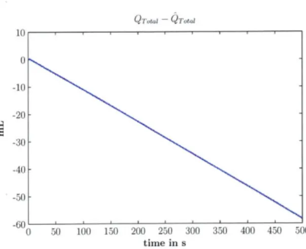
The CVSIM model described is a closed system with no external sources or sinks of charge: the amount of charge in the model is completely defined by the initial conditions and must remain constant throughout the simulation. However, when the model was implemented with the state variables as described by Equations 2.6 - 2.11, volume conservation was not observed (see Figure 2-3).

Deviations in volume were being caused by numerical errors associated with the time-varying derivative terms (dC(t) _{dt dt}, C(t) , see Equations 2.6 and 2.9). Figure 2-2b shows a plot

of the derivatives of the compliance functions for one cardiac cycle. The derivatives are not well behaved in that they vary dramatically over short periods of time when transitions oc-cur from systole to isovolumetric contraction, and from isovolumetric contraction to diastole. The abrupt changes in the ventricular compliance derivatives lead to numerical integration errors when computing ventricular pressures. Moreover, the magnitudes of the ventricular compliance derivatives are relatively large which further magnify the numerical errors. A simple fix to this problem is a change of ventricular state variables to volume, instead of pres-sure, which removes the dependency on the ventricular compliance derivatives. Equations 2.26 - 2.27 represent the revised state equations for the ventricles.

dQ 1 = - 10

(2.26)

dt

dQr

dt - (2.27)

Figure 2-4 shows a time-series plot of the deviation in expected and calculated total blood volume after the change of ventricular state variables. Barring insignificant numerical errors, the change of state variables leads to volume conservation.

QT10~l QTti 10 0 -10- -20- -30- -40- -50--60 0 50 100 150 200 250 300 350 400 450 500 time in s

Figure 2-3: Difference between expected total blood volume (QTotal) and calculated total blood volume (Q otal), with left and right ven-tricular pressure (voltage) as state variables.

6 x10-2 - Qmtal 4- 2-0 -2 -4--6 -8 0 50 100 150 200 250 300 350 400 450 500 time in s

Figure 2-4: Difference between expected total blood volume (Qrotal) and calculated total blood volume (QTotal), with left and right

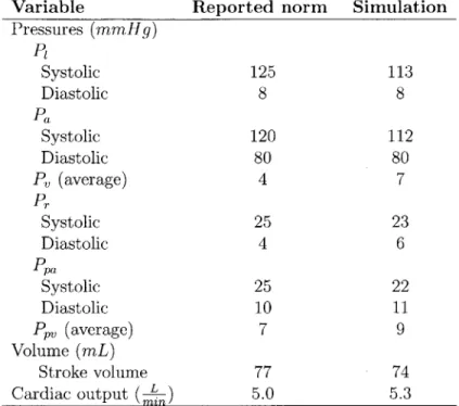
Table 2.2: Comparison between model outputs and reported norms for compartmental pres-sures, stroke volume and cardiac output.

Variable Reported norm Simulation Pressures (mmHg) P Systolic 125 113 Diastolic 8 8 Pa Systolic 120 112 Diastolic 80 80 P, (average) 4 7 Pr Systolic 25 23 Diastolic 4 6 Ppa Systolic 25 22 Diastolic 10 11 PPV (average) 7 9 Volume (mL) Stroke volume 77 74 Cardiac output (

)

5.0 5.3

2.3.7

Model Validation

The ability of the CVSIM model to reasonably represent the underlying physiology can be gauged from a comparison of the model outputs, at different time scales, to what is generally observed in humans.

Beat-to-Beat comparisons

Table 2.2 shows a comparison of steady-state cardiac output, and beat-to-beat pressure values and stroke volume. The norms listed are for a 70-kg adult as reported by Milnor in

Mountcastle's Physiology [20, 21].

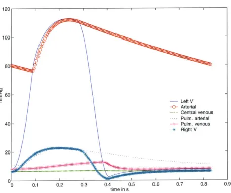
Pulsatile Waveforms

The validation of the intra-beat dynamics is made by plotting the pressure waveforms for all the compartments. Figure 2-5 shows the plots for all the compartmental pressures for a single

60

40

20

0 0.1 0.2 0.3 0.4 0.5

time in s 0.6 0.7 0.8 0.9

Figure 2-5: Pulsatile pressure waveforms for a single beat.

beat. On average, the pressure waveforms look similar to the actual catherized data. The pressure magnitudes and time-constants involved seem reasonable, thus validating the choice of parameter values used. However, expected differences, such as the absence of reflected waves due to the lumping of parameters, are visible.

2.3.8

Interstitial Fluid Compartment

Body fluid is divided into two distinct categories: intracellular and extracellular fluid. As the name suggests, intracellular fluid consists of the volume within the cells which forms approximately of the total body fluid. Extracellular fluid is further divided into interstitial

fluid and blood plasma. The division is such that in steady state, 14 of the extracellular

volume resides in the interstitial space, whereas the rest is blood plasma. Figure 2-6 shows the distribution of fluid volume for an average 70-kg adult.

E E - _{Left V} -0- Arterial - Central venous - Pulm. arterial -+- Pulm. venous * Right V -...-.. I 1jf1 I I 100 80C

Figure 2-6: Volume distribution for an average 70-kg adult. Approximately 60% of body mass is fluid. This percentage can vary depending on age, sex, and obesity [2].

The fluid in plasma constantly interacts with the interstitial space through the capillary pores, however, the CVSIM model does not represent this communication. In steady-state, the absence of the interstitial compartment does not significantly inhibit the ability of the model to represent the underlying physiology, as no net exchange of volume takes place between the two compartments. However, during disease conditions, such as hemorrhage, or during clinical interventions, such as administration of fluid boluses, the role of the in-terstitial compartment becomes significant. In this section, we describe the addition of the interstitial fluid compartment (int), and we detail the derivation of the nominal parameter values associated with the compartment. 2

Model Addition

The interstitial fluid compartment is represented by an additional resistor and capacitor

(Rint, Cint), connected between the systemic arteries and veins (see Figure 2-7). The

ca-2

Note: The interstitial compartment is used only in Chapter 5, when matching simulated data to actual patient data.

pacitor models the volume storage ability of the interstitial fluid space, whereas the resistor models the resistance faced by the fluid when diffusing between the two compartments.

The nominal value for Cint can be determined using the following logic, which analyzes the fluid dynamics before and after the administration of a fluid bolus 3 (saline, for example): " In steady-state, P, = Pint, as no net exchange of volume takes place. Consider an

initial (i) steady-state where Pj~n = P, = P.

" After intra-venous administration of a fluid bolus

AV,

a new steady-state will be reached where

I

of the bolus volume will diffuse into the interstitial space, whereas 14

14 1

will remain in the circulatory system. Since the veins form the largest blood reservoirs of the circulatory system (storing 64% of the volume [2]), 64% of the fraction of the bolus volume remaining in the intra-vascular space will reside in the veins once the new steady-state has been reached. As compartmental pressure can be expressed as a ratio of volume to compliance (see Equation 2.1), the following set of equations is obtained when equating the final (f) steady-state pressures Pft and P:

Pf4 = Pf 11 1 3 1 P + -AV. - =P

+

-

AV

-64

%*c

14 Cint 14 CG 11 14 100 14 3 64 Using the nominal value

Cv

= 100 m , Cint ~ 573 L L

mmHg' mmHg

We use the the same analysis, which considers the dynamics after the administration of a fluid bolus, to determine the value of Rint. The nominal Rint value can be resolved using the time-constant involved in the transfer of fluid volume between the interstitial space and the circulatory system. Based on an extensive literature review, Heldt determined that the time-constant for diffusion to and from the interstitial space is the same, with a nominal

3_{We assume the administration of isotonic fluids which redistribute between the intravascular and} inter-stitial spaces only [22].

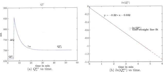
Q av ougigQav incoming qr (t) p_ (t) qt) qa t Pa(t) q10(t) R. Ra CV P. (t) t Ca Int C.-_Cint qint (t)

Figure 2-7: Addition of the interstitial compartment between the systemic arteries and veins.

value Tit = (4.6 ± 0.4) min [5].

In the circuit representation of the model, the topology is such that the venous charge decay (post-administration of a fluid bolus) does not follow a simple RC time-constant. Therefore, it is not trivial to determine an analytical formula for the time-constant which can be used to pinpoint the exact

Rint

value. To overcome this problem, we assume that on a beat-to-beat averaged basis during the transient, the charge flowing in from the arterial side (Q" coming) is offset by the charge flowing into the right ventricle

(Q"j

₀

i

-₉

,

see Figure 2-7). With this assumption, the added venous charge redistributes itself between C, and

Cint,

which are connected in series through Rint. This configuration leads to the following

approximate value for Rint:

Tint = 276s

Rint. = 276s

Cv + Cint Rint ~ 3.2PRU

Next, we carried out several simulations of fluid bolus administration in which Rint was varied around its approximate value of 3.2 PRU. Based on simulation results, Rint = 2.3 PRU yielded a venous charge decay time-constant of approximately 4.5 mins. Hence, a nominal value of 2.3 PRU was assigned to Rint. Figure 2-8 shows the plot of simulated venous volume vs time which captures the dynamics induced by a fluid bolus administration. Figure 2-9 shows a plot of the difference between Q

ncoming

and

Q'Vtgoing.

We observe that

gZG 0 0 n(Q'V

-0.2 y = -0.22 * x - 0.032

850---0.4

800 -0.6- n s'straight line fit

750 - A

-0.8-Tint a-1

700

1.2

--6500 10 20 30 40 50 60 -1.4

time in min time in m

(a) QgV VS time. (b) ln(Q'v) vs time.

Figure 2-8: Beat-to-beat averaged venous charge (Q'v) vs time. Sub-figure (a) shows the plot of

QaV

vs time before and after the administration of a fluid bolus. Sub-figure (b) shows the plot of ln(Qav) vs time, and its best straight line fit, after the administration of a fluid bolus. The time-constant for the charge decay is the reciprocal of the slope of the best straight line fit:

rint

~ 4.5 min.

this difference is indeed small compared to the venous charge decay. Thus, the assumption we made in approximating a value for Rint is verified to be reasonable.

The addition of the interstitial fluid compartment adds another state variable to the model. See Appendix A for the details of the new model equations.

2.3.9

Concluding Remarks

Though the CVSIM model does not capture the fine details of cardiovascular function, it is a reasonable model to start investigating the use of parameter estimation as an aid in patient monitoring. Since the average behavior of the model is similar to the underlying physiology, there is credibility in the use of the system. However, various additions to the model have been proposed, including the use of inductors to model the inertial effects of blood [11]. Moreover, the systemic circulation has also been modeled as a distributed set of parallel compartments, as opposed to a single compartment, in order to include the

Qq av zncomning Qavout going 0.4 0.35 0.3 0.25 0.2 -0.15 F 0.1 u.Ud 0 5 10 15 20 25 30 time in min

2-9: _2-'incoming Q ,v , -

Qav

outgoing after the

individual effects of prominent arteries and veins [5]. Nevertheless, there is a clear trade-off between model complexity and ability to represent minute details. The CVSIM model strikes a healthy balance by providing a system which is of manageable complexity, and reasonable in its ability to represent the cardiovascular system.

Figure bolus.

35 40 45 50

administration of a fluid

'

Chapter 3

The Cardiovascular Control System

The cardiovascular system forms the lifeline for cell survival as it transports oxygen and nu-trients. Entrusted with such a mammoth responsibility, cardiovascular function maintains homeostasis by adapting dynamically to meet the current needs of the body and to coun-teract hemodynamic perturbations. For example, in the absence of a control system, the commonplace act of regaining the head-up posture from a supine state causes the blood pres-sure at the level of the heart to drop to such a degree that one might faint. In the presence of cardiovascular control, however, changes in posture are activities that we perform seemingly effortlessly without even noticing the stress that we impose upon the cardiovascular system. In order to accomplish its task, the cardiovascular system exerts control at both local and global levels. Local control includes the modulation of vascular resistance by tissue beds to maintain adequate blood flow in a specific region. Global control, on the other hand, involves the regulation of hemodynamic variables to maintain overall pressure. The reflex mechanisms involved in employing control span many time scales, from the fast neurally-mediated (seconds to minutes) to the slower hormonally-neurally-mediated (days)

[2].

In order to faithfully track patient state continuously, we are interested in modeling the short-term cardiovascular control to clinical interventions and to changes in the degree of a disease condition. In this chapter, we describe the arterial baroreflex, which is a princi-pal component of short-term neurally-mediated control, and we outline its implementation.

Furthermore, we qualitatively validate the baroreflex function by simulating certain disease conditions.

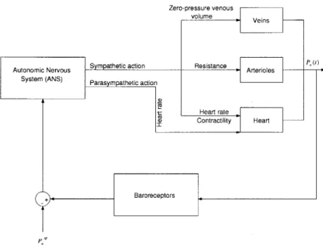
3.1

Arterial Baroreflex

The arterial baroreflex is a negative feedback system that aims to maintain ABP around a particular set-point. The afferent leg of the system includes pressure sensors, known as baroreceptors, located in the aortic arch and the carotid sinuses. These receptors sense ABP and transmit this information via afferent fibers to the brain where the deviation in ABP from the set-point is mapped to sympathetic (a and 0) and parasympathetic activity. Increased a-sympathetic action leads to increased peripheral resistance and decreased zero-pressure venous volume, while increased -sympathetic action causes an increase in cardiac contractility and heart rate. Parasympathetic action affects the heart rate in a manner opposite to /3-sympathetic action; an increase in parasympathetic activity reduces the heart rate instead of increasing it. Figure 3-1 presents a block diagram of the arterial baroreflex system.

Our representation of the arterial baroreflex is based on Davis's extension of deBoer's work [4, 23] with certain changes in implementation that are described in the next section.

3.2

Implementation

Previous implementations of the baroreflex mechanism adopted relatively coarse time-steps for the control system as compared to the rest of the cardiovascular model [4, 16]. It was deemed computationally inefficient for the reflex system to react to every sample of ABP, as pulsatile ABP is bandlimited at frequencies below ten times the mean heart rate, while the frequency response of the cardiovascular regulatory mechanism is bandlimited at frequencies less than the mean heart rate [16]. Thus, in Davis's model of the baroreflex, pulsatile ABP was averaged over 0.5 s and then sampled at 0.5 s

[4].

This implementation, however, leads to aliasing as the frequency content above 1 Hz is not sufficiently filtered by the 0.5 s running

Zero-pressure venous volume - _Veins

Autonomic Nervous Sympathetic action System (ANS) _{Parasympathetic action}

ao

I

a(D Resistance _Arterioles Heart rate Contractility Heart + Baroreceptors

Figure 3-1: Block diagram of the arterial baroreflex system. that the system is aiming to maintain.

PfP is the set-point pressure

average filter. A subsequent implementation by Mukammala [16] averaged the pulsatile ABP over 0.25 s and then sampled it at 0.0625 s, thus reducing the aliasing effects. In order to completely remove the effects of aliasing, we decided to implement the control system in continuous-time.

3.2.1

Preprocessing and Error Calculation

Since the cardiovascular regulatory mechanism responds to low-frequency fluctuations of ABP from a set-point, the pulsatile ABP signal is first low-pass filtered to remove the strong frequency content at, and above, the mean heart rate '. Next, the low-pass filtered ABP signal (Plp(t)) is subtracted from the set-point to produce the error signal (e(t)), which

'In principle, the low-pass filter should not be required as the physiological control system response itself is bandlimited at frequencies below the mean heart rate. However, as shown in Section 3.2.2, the response of the estimated control system does not sufficiently attenuate the strong, high-frequency content present in the ABP waveform.

P P (t)

D.Low-pass filter + Non-linear mapping

Figure 3-2: Block diagram depicting the preprocessing involved.

then is passed-on to a non-linear mapping block that represents the baroreflex saturation characteristic [24]. As the autonomic nervous system exhibits a limiting behavior in action,

the following mapping is applied to e(t) [23]:

e(t)

esat(t) = 18 arctan( ) (3.1)

18

This mapping restricts the input to the effector mechanism to approximately ±28 mmHg. Figure 3-2 illustrates the preprocessing mechanism.

3.2.2

Effector Mechanism

Control Filters

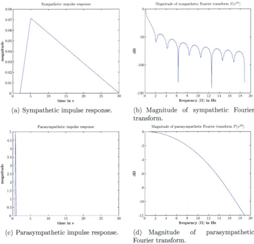
The effector mechanisms are modeled as a linear combination of two LTI filters which rep-resent the sympathetic (a and /3) and the parasympathetic limbs of the autonomic nervous system. The filters are defined by their unit-area impulse responses, s(t) (sympathetic)

and p(t) (parasympathetic). Figure 3-3 illustrates s(t) and p(t) along with their Fourier

transforms.

The filters were implemented using Simulink's continuous-time blockset which allows for the representation of rational transfer functions and continuous-time delays. The transfer