HAL Id: hal-00374105
https://hal.archives-ouvertes.fr/hal-00374105
Submitted on 7 Apr 2009
HAL is a multi-disciplinary open access
archive for the deposit and dissemination of
sci-entific research documents, whether they are
pub-lished or not. The documents may come from
teaching and research institutions in France or
abroad, or from public or private research centers.
L’archive ouverte pluridisciplinaire HAL, est
destinée au dépôt et à la diffusion de documents
scientifiques de niveau recherche, publiés ou non,
émanant des établissements d’enseignement et de
recherche français ou étrangers, des laboratoires
publics ou privés.
Trail Systems as fault tolerant wires and their use in
bio-processors
Nicolas Glade, Hedi Ben-Amor, Olivier Bastien
To cite this version:
Nicolas Glade, Hedi Ben-Amor, Olivier Bastien. Trail Systems as fault tolerant wires and their use in
bio-processors. Modelling Complex Biological Systems in the Context of Genomics, 2009, pp.85-119.
�hal-00374105�
Trail Systems as fault tolerant wires and their use in bio-processors
Nicolas GLADE† ∗,Hedi M. BEN AMOR† ,Olivier BASTIEN# † TIMC-IMAG Laboratory, UMR CNRS 5525,
University Joseph Fourier, Faculty of Medicine of Grenoble, 38700 La Tronche
# INRA - PCV, CEA Grenoble,
17 Av. des Martyrs, 38054 Grenoble
February 17, 2009
Abstract
Motivated by the idea that one day, probably far in the future, the computers and robots will be architec-tureless, made of collections of numerous ’intelligent’ subsystems or nanomachines able to self-organize each other into computational morphologies with perhaps more computational power than classical electronic-based computers, many studies are burgeoning in different fields (chemistry, biology, condensed matter, quantum physics, ...). Several systems inspired from Nature have indeed been proposed yet for designing unconventional computer architectures using processing modes of various nature and at different scales.
The heterogeneous set of natural or artificially designed systems called trail systems, commonly asso-ciated to self-driven particles (agents1) with tropistic activity (through a communication based on traces
let in the environment), is a soft matter with self-organizing properties sufficiently robust and fine for de-signing biocomputing structures. In this context, individual trails systems could be viewed as single wires and logical gates in a self-organized bio-processor, in the same manner axons are connecting the neural nodes in a neuro-processor. Their efficiency as wires depends on their specific properties which are often related to their scale. The robustness of their self-organization at the microscopic scale level occurring in a noisy environment, can be studied by a model based on effective computing systems (i.e. Turing machines) programmed to behave first as deterministic and perfect trail systems, then as stochastic-working trailing agents subject to randomness.
Key words: Trail systems, Self-organization, Ant-based model, Robustness, Biocomputing, Bio-wires
∗Contact. Tel. +33 (0)4 56 52 00 26 – nicolas.glade@imag.fr
1
Introduction
It is obvious for most scientists that natural systems possess indeed that potentiality to compute things. Nevertheless biocomputing approaches are often very difficult since the researchers block in implementing effective computational calculi with their system of interest. In other terms, it is easy to imagine the possible computational power of a biological system but one can not calculate easily ’1 plus 1’ by using molecules, living cells or other natural systems, unless applying to those system a strong control at the expense of the real potential of these systems (self-organization capabilities notably). Moreover, in comparison to electronic based processors that have a deterministic behavior and whose structure is well defined, natural systems are on the contrary very subject to noise, show stochastic fluctuations to dramatic changes in their behavior, and are poorly structured. In addition, their structuring is non-permanent compared to silicon based hardwares. These two point were largely analyzed by M. Conrad – died in 2002 –, one of the most prolific fathers of the notion of ’molecular computing’ (1, 2).
In this article we bring close together a class of self-organizing natural systems, the trail systems, and effective programmable systems such as Turing machines whose behaviors are well known.
Natural systems are in general noisy and tend to the extend of their entropy. However some of them self-organize either by static mechanisms (e.g. liquid crystals) or by dynamic dissipative processes as it is the case in almost all biological systems, e.g. the organization of cells from tissues to organisms, population dynamics, or trail systems. By a permanent consumption of energy (or matter, such as reactive compounds), the latter self-organize over space and time and maintain their order to low entropy levels (compared to the entropy corresponding to a total disordered distribution of their constituents) (3, 4). Self-organization of the so-called dynamical systems, or collective systems, always occurs at a macroscopic level compared to the microscopic level at which their components act. It is due to the combination of the numerous individual actions of the microscopic constituents, or agents (e.g. animals, cells, molecules), and the communication between them that synchronizes those individual actions. In that, they get closer to effective programmable processors than other natural systems like disordered solutions of molecules.
Processors are arrangements of wires and elementary signal integrators such as logical gates in elec-tronic processors or neural nodes in neuro-processors. Specialized processors are programmed structurally. This means that one architecture computes a given input signal according to only one program. This is the case for the neuro-processors once their organization is fixed, or for some electronic chips dedicated to one computational task. Moreover, some processors, like those we use in our computers, can be also programmed dynamically. Their architecture is designed for a general use. Applying on the architecture a set of instruc-tions as the computing process goes along (in other terms a program) corresponds to its refinement (and a dynamic adaptation).
Among bioprocessors, neural networks are not the only natural or bio-inspired processors that are able to learn or change a configuration and to self-adapt to a given context so as to process the information differently. Biological regulatory networks are very often subject to changes of external (environmental) or internal (intracellular) conditions, so they have to adapt so as the cells or organisms can survive. Biological feedbacks and feed forwards act as activators or inhibitors of biological pathways (e.g. sequential cascades of reactions), respectively in the past or in the future of the biochemical process trajectory. A learning bio-processor based on microtubules and motors self-organization has also been proposed by Pfaffmann and Conrad (5). In this model, microtubules are assumed to be able to transport the signal in an electric form (nb. it is important indeed to highlight the importance of the difference of nature between the constituents of the processor and that of the signals that travel through its wires and gates for being treated). Starting from a solution of microtubules and linker molecules (such as molecular motors), a reticulated morphology forms and constitutes the architecture of a certain processor. Used for processing a certain input, it returns an output. The latter is compared to a reference (calculated differently) and adjust progressively the architec-ture of the microtubule-based processor by changing the level of reticulation. If the processor computes well, the architecture freezes ; if not, the architecture is warmed and changes. Such microtubule-based processors are plausible given the subsequent results that concern the control of their self-organization with linkers or motors (6, 7) and by admitting the concept of information transfer and processing inside – or at the surface of – microtubules, largely defended by several authors such as Hameroff (8–10), Tuszinsky (11, 12) (who also made recently calculations of ionic waves propagation along actin fibers), or other authors more recently (13, 14).
The plasticity of a neuro-processor compared to an electronic one is another important point to keep in mind. If the latter can be dynamically programmed (after being designed and structured by engineers over several years of successive ameliorations), the structure of the former can be reconfigured both by physical changes in the set of connections and by adaptations of its weights and thresholds (which in real neural networks found an equivalence in the increase or decrease of the number of available receptors to neurotrans-miters or in the increase or decrease of the number, shape and volume of sensing areas, i.e. dendritic spines). That way, by a learning process that compares for a given set of entries the result with a reference (professor), neural networks can reconfigure into different neural-processors. Since all neurons can potentially connect to all the others in the network, including themselves (in particular in formal networks), and given their
high reconfigurability, their structural combinatory is largely higher than that of electronic programmable processors. Plasticity is a advantageous feature of formal neural networks, but this also occurs within the brains when we learn a better or different manner to proceed for doing something. After an accident that destroyed a part of the brain or after some surgical resections, other parts can also reconfigure to reestablish the function lost. On the other hand, one must accept that such a processor is not optimal, in particular when the number of neurons implied is very important.
Neural networks are not the only natural or bio-inspired processors that are able to learn or change a configuration and to self-adapt to a given context so as to process the information differently. Biological regulatory networks are very often subject to changes of external (environmental) or internal (intracellular) conditions, so they have to adapt so as the cells or organisms can survive. Biological feedbacks and feed forwards act as activators or inhibitors of biological pathways (e.g. sequential cascades of reactions), respec-tively in the past or in the future of the biochemical process trajectory. A learning bio-processor based on microtubules and motors self-organization has also been proposed by Pfaffmann and Conrad (5). In this model, microtubules are assumed to be able to transport the signal in an electric form. Starting from a so-lution of microtubules and linker molecules (such as molecular motors), a reticulated morphology forms and constitutes the architecture of a certain processor. Used for processing a certain input, it returns an output. The latter is compared to a reference (calculated differently) and adjust progressively the architecture of the microtubule-based processor by changing the level of reticulation. If the processor computes well, the architecture freezes ; if not, the architecture is warmed and changes.
We think that self-organized trail systems can be considered for structuring bioprocessor fine architec-tures and can work as neural networks do. Although they are less robust than electronic circuits or even neurones, they are however able to reconfigure more rapidly. Moreover, they sometimes make some errors. Errors confer a great advantage to collective systems : when some individuals behave differently to the mass, one would say they make errors, others would say they explore other potentialities. The well known example is the determination of the best pathway among several paths that join together two points (e.g. the nest and a food source) by a population of ants (15, 16). By collective dynamics based on the release and the sensing of pheromone trails by individual ants, the ant colony determines progressively the best pathway, but some of the ants – that we will call ’explorers’ – fail in following the principal track and use another pathway. If the better one is blocked by an experimentalist (or by an environmental accident such as a rockfall or due to flooding) the secondary options that has already been found by some ants are rapidly used. In the case of ants, the exploratory trajectory is mostly random but can be enhanced by other external factors (smells, geometry constrains of the landscape ...). Then, moving to other pathways is something easy for the colony since the explorers have found yet these new pathways. The rest of the colony just has to follow their tracks (i.e. pheromone trails). By this way, the colony can also discover other sources of food (resources in general) or new territories for settlement.
Very few – but successful – attempts were done that showed that NP complex problems such as network routing problems are perfectly and more efficiently resolved when based on trail processes (as shown with the use of virtual ants by Bonabeau et al (15)). The different systems that belong to this heterogeneous set are well studied independently now. Nevertheless they have surprisingly never really been viewed more theoretically as a unique family of systems sharing the same properties and studied as it is, as a generic model described by a unique set of parameters for each TS-agent and its trail. Neither have they really been studied for their computational properties. In the best case, they are considered in a simplified manner as multi-agent systems (17), but this does not take unfair advantage of all their characteristics.
Trail systems possess however very interesting characteristics in terms of computational efficiency and control. Their ability to produce preferential tracks and to follow – or be influenced by – them results in the emergence of temporal and/or spatial order and forms. That way, the whole system behaves naturally as a self-organizing dynamical network (a sort of circuitry where cables are defined dynamically) that can – when perturbed by external factors acting globally on the whole system or locally in the form of perturbing nodes (e.g. food sources, poison, walls) – re-adapt to take into account the new geometry and features of the system in its environment. Moreover the structurability of such systems is intrinsically high due to their structural aspect and to their self-organizing properties, and it can be enhanced by a direct control of the dynamics and the orientation of the TS-agents. The majority of biocomputing researches based on multi-agents use them directly as processors so that their concerted actions in a given context (inputs) di-rectly gives a morphological result. This biocomputing approach is very interesting for solving optimization and organization based problems. This is for example what is done in collective robotics (17) or internet routing problems (15). Another manner to proceed is indirect : this time, the agents are used to construct a – very reconfigurable – processor architecture that is used afterwards for computing classical calculi (and whatever problem a classical electronic processor can compute). As for a neural network, such a trail sys-tem based network would then be able to learn a configuration that, stimulated by some signal of different nature (e.g. light, electricity ...), would process it such as it corresponds to the expected computation. This would be facilitated and enhanced by using TS-agents of fibrillar nature, i.e. the orientation of cytoskeletal supramolecular assemblies under the action of electric or magnetic fields (18–21).
The properties of trail systems allow us to better identify them to structurally programmable processors compared to classical reaction-diffusion systems (e.g. see (22) or (23) for BZ-based computing which needs
either a strong control of the BZ reaction by local light inhibiting stimuli or by using a fixed geometry for the gel in which the reaction is realized), particularly in the case of fibrillar trail systems. We propose here to browse through those properties and computational interests that depend on the nature and the scale of those systems, and on the influence of their environment. In this article we also present the first step of a research agenda, i.e. a model based on an analogy between individual trail systems and wires or connections of an electronic processor or a neural processor. The model is an automaton very similar on its form to a Turing machine where the TS-agent is programmed to release traces of its trajectory in the environment, and for using them, but subject to intrinsic error or stochasticity coming from the environment. In that very simplified model of trail system, we identify clearly all sources of stochasticity that can affect the behavior of TS-agents, thus allowing us to study the robustness of their spatial self-organizing ability due to their microscopic –individual – properties. We also discuss of what ensures the robustness of self-organization at the level of a population. In particular, we are interested in the manner information is shared between TS-agents, and discuss on how such transfer entropy can be measured in our model or how it could be done is real systems. Finally, we describe how a learning process similar to that used for configuring formal neural networks will allow to obtain well structurally programmed trail-system based processors. It is interesting to note that an evolutionary process unifies the couple engineer-processor in a feedback loop : the engineer (that is also able to use feed forward decisions), creates a processing chip and tests it until it realizes the expected task or calculus. Evolution played the role of the engineer in natural systems (this point has been largely highlighted in several papers (24, 25)). Actually, the properties of the natural trail systems (as those cited above) have been selected – in a Darwinian sense – so as the robustness of the self-organization depending function is ensured in respect to the features of the natural environment.
2
Characteristics of the trail systems
Trail systems are constituted of numerous active elements in interaction in their environment. These ele-ments are composed of two distinct parts : an active agent (TS-agent) and a trail.
The TS-agent is an object perceived as a unique physical entity. It has its own rules of behavior: in-ternal rules that describe the changes intrinsic to this entity (independently to exin-ternal actions), and rules that allow it interacting with other TS-agents, with its surrounding environment or with external fields. Compared to the TS-agents, the trails are not precisely defined and are not really limited physically until a molecular description. They are made of local variations of the environment. Those variations have a maximal intensity at their sources, the TS-agents, and spread out or are progressively degraded from the instant they are generated. Their description is very related to level of abstraction used for describing the matter that constitutes the environment : a discrete manner or a continuous one. Viewed from a macro-scopic point of view, one can mark a trail out with a certain accuracy, but the precision of their frontier is limited by the sensitivity of the experimentalist to the variations observed. Moreover when the scene is magnified, the observer can distinguish the different components of the trail, showing that the trail is not in the form of a unique coherent entity. Nevertheless the latter can drive the self-organization of the agents at the macroscopic level.
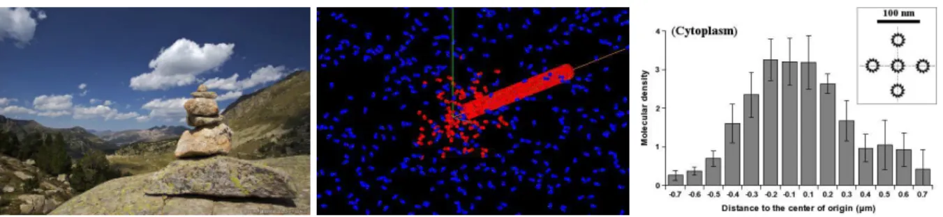
The trails can be of various nature (chemical traces, physical tracks, hydrodynamic trajectories...) and have different effects (causing activating or inhibitory behaviors). Animals like social insects (16, 26, 27), marine snails (28), birds or flying drones (29), or human pedestrians (30, 31) or mountaineers (fig. 1 left) take advantage of this process for self-ordering and optimizing tasks, particularly path finding, hunting or foraging, thus saving energy. Other, such as harbor seals (for fishing activities)(32), ’know‘ how to use the trails produced by other systems for profiting from the same properties. All are macroscopic very efficient trail systems. Their efficiency is important in the sense that this mode of communication has a real influence on the synchronizing activity or the self-organizing behavior of the TS-agents that compose the system. Mi-croscopic ones exist such as chemotactic cells (33) or bacteria such as actin comet systems (e.g. actin comets produced by TS-agents such as the Listeria or Shigella bacteria, or Arp2/3 -coated latex beads (34, 35)), but also molecular ones such as the self-assembled biological fibers (e.g. microtubules or actin filaments) (fig. 1 right) or artificial DNA-designed programmable nanotubes (36) and carbon nanotubes (37). In simulated systems such as the Conway’s game of life or the Langton’s ants (38), they are often called ’puffers‘, i.e. self-maintained gliders that produce persistent trails of numerical nature (e.g. a trajectory composed of cellular automata cells filled by active states). For example a chemical trail, such as those made of pheromones that drive ant colony dynamics, is composed of numerous individual molecules that one could distinguish individually by a accurate observation at the ’nanoscopic‘ level. The same observed without or only at low amplification would be viewed as a macroscopic object, correctly defined along a certain area emerging from the source, and becoming progressively fuzzy at its undefined border. The quality of the frontiers observed depends on what the observer can perceive, as to say on its sensitivity to the signal that constitutes the trail. If the molecules that compose the trail are stained by a fluorescent marker, it will depend on the sensitivity of the experimentalist’s camera to the light emitted. However evident it may be, that remark is the same for the TS-agent which is sensible to the trail signal only beyond a certain threshold.
Figure 1: Traces let by natural trail systems. (Left) A cairn in the pyr´en´ees in France (used by permission of P.-H. Muller, http://www.boreally.org/). One cairn constitutes an isolated element of the human trail signal clearly visible by humans over the landscapes. (Center) Model of disassembling microtubule (see (39)). Here, the microtubule shrinks at the unrealistic rate of 2000 µm.min−1 so as we are able to observe the formation of a tubulin-GDP trail (red molecules ; blue ones are tubulin-GTP). At realistic rates (¡20 µm.min−1) no anisotropic trail forms and the heterogeneity observed is very weak as shown on the diagram to the right. (Right) Measurement from a simulation of the amount of tubulin-GDP released by disassembling microtubules in solution. Data correspond to the density profile of tubulin-GDP around the tips of disassembling microtubules, measured from the center of an array of 5 motionless microtubules (see the inset showing a transverse cross section of the x axis and of 5 MTs), each of them respectively separated by 30 nm (one microtubular diameter). All microtubules disassemble simultaneously at 20 µm.min−1 (1.85 ms.heterodimer−1) which is a quite fast disassembling rate. The macroscopic diffusion rate of individual tubulin dimers corresponds to that measured in the cytoplasm (5.9 10−12m2.s−1)(40). The quantity of tubulin-GDP molecules liberated is very low and needs to be integrated in time for obtaining average profiles. The graphic has been reconstructed by integration of the density maps of 6 independent simulations, during 1.8 ms (i.e. the average time separating the liberation of 2 tubulin-GDP molecules by a disassembling microtubule), between the simulation times 9.2 ms and 11 ms, along the 3 axis (a total of 6642 profiles)
and thereby that of the resulting self-organizing processes. Considered aside, the system has a certain ef-ficiency in processing information and self-ordering that can be inferred from the parameters enumerated below. What is the most important is nevertheless that the information generated and processed by such TS-agent – trail elements must be discriminated from the other interactions and processes (e.g. mechanical interactions, noise and thermal agitation, convection or flows, other concurrent reactions ...) that occur in the same time in their direct neighborhood. The importance of a hierarchy in information processing systems and in particular in natural systems has been largely described by Conrad (2) : all interactions are processing events but all occur at different time and space scales, some of them being negligible in comparison to others that exist at the time and space scale level we are interested in. In our case, we are interested in trail system based processing and not in the possible different processing modes that could exist at a molecular level between some of the molecules or atoms that compose the system (as it is used in the hypothesis of information processing inside microtubules or actin (8–14)). An enumeration of the common parameters sufficient to describe whatever trail system and necessary for trail-based processing is given below. TS-agents :
● Panel of actions (rules) available. All TS-agents are random walkers since they generally can’t
’see‘ directly the trail they follow (except perhaps in the particular case of animal pathways that can be directly viewed by the TS-agent before it encounters physically the trail). Once a trail is encountered, the internal state of the TS-agent is modified. Its internal rules take this new state into account so as the individual behavior of the TS-agent is now modified. In particular those changes induce an ’active searching’ of the trail pathway by the TS-agent. Such ’intelligent‘ actively searching TS-agent are considered usually as active walkers but that notion is very imprecise : we can perfectly understand this meaning in the case of animals for example. It is more fuzzy in the case of cells or bacteria, and worth for pure molecular systems like biological fibers. The moving biological fibers encounter on their trajectory variations of composition and concentration in the medium, formed by the accumulation of numerous fuzzy, weak and extended trails (in this case, one may better say ’molecular clouds’ instead of ’trails’). This affects the reactivity at their ends. When growing in favorable regions of the solution their growth is statistically enhanced and, on the contrary, when encountering unfavorable chemical compositions they can start to shrink or pause. They however can’t reorient for following chemical trails as ants do. Nevertheless, a progressive process of selection – by a succession of growth, shrinkage and nucleation of new fibers – can lead to the selection of preferential orientation of the fibers. Despite a clear difference of efficiency, this process can be also assimilated to an active searching when considered
from an upper level of observation.
● Sensitivity to the trail. The most important point is the efficiency of the TS-agent – trail recognition
(or the attention of the TS-agent to the signals let by others in the environment). As evoked before, the TS-agent – an animal, a cell, a supramolecular self-assembly – reacts to the signal contained in the trail structure only beyond a certain threshold. All TS-agents possess a sensing zone or a preferential region for physical interactions with the environment or for chemical ligand dependent reactions that can be assimilated to sensors (e.g. sense organs for animals, chemical receptors on a cell, reacting ends of biological fibers). The threshold is a combination of both the surface of recognition (reactive surface of the agent), the density of the sensing elements present on this surface (e.g. individual molecular receptors) and their individual affinity or sensitivity. Actually, it is the size of the surface of recognition on the TS-agent compared to the size of the trails encountered that is important. For better efficiency, and at least a better directional symmetry breaking, the trail must be thiner or of the same order of this region (i.e. of the TS-agent if the region is more or less confounded with the entire individual). For example, let us consider two cases : (i) the ant and (ii) the microtubular systems. In (i) the trail is thin and long, and the TS-agents are approximately as large as the width of the trail (about 1-5 mm). Such an anisotropy leads to a strong local symmetry breaking along the trajectory of the TS-agents and although the ants walk randomly, they are permanently biased in a preferential direction, often crossing the trail they follow and aiming to come back to it. This behavior is not unreminiscent to what occurs in human pathways and ’cairns’ where those traces are very visible by the mountaineers, often over large distances, that way drawing kind of discrete tracks (fig. 1 left). On the contrary, in (ii) the trail produced by a microtubule is very extended (over microns) much more larger than the size of the ’sensor‘ of the fiber (30 nanometers) (see (39) and fig. 1 center & right). In that condition, this actions of the agent can not be biased in a preferential direction since the agent is included in the trail and can not cross it. The only possible effect of microtubule trails (and consequently of actin filament trails also) occurs at the level of huge populations of fibers at the millimeter scale, when macroscopic variations (compared to the size of the agents) of tubulin composition appear and cause massive synchronized reactions of the fibers, that are transmitted by diffusion. This is observed in solutions of microtubules in highly reactive conditions, as spatio-temporal variations (propagating waves) of the concentration of microtubules (41).
● Moving rate of the TS-agent. The motion of an agent has two origins : a motion that it controls
due to its own dynamics, and a motion induced by external factors such as external fields, flows and diffusive motion. Their displacement relative to the environment will affect the manner the TS-agent will sense the fluctuations of the medium. It depends actually on the ratio between the rate (efficiency) of recognition of the fluctuations by the TS-agent, and its moving rate. Moreover, the effect of the external factors on the TS-agents will strongly condition the success of specific trail-based processes, particularly when they are of the same order of the characteristic motion of the TS-agents. If animals are very weakly sensible to normal external factors (ex: wind) that’s different for cells subject to flow or convective motions, and worth for biological fibers subject to strong mechanical effects and thermal agitation.
● Internal memory. When TS-agents evolve in their environment they are stimulated by the trail
signals and other external factors. This modifies their internal state at least for a certain duration after stimulation. Animals have their neurons activated for an active searching of trails ; particular pathways of the metabolic-genetic network of the chemotactic cells or bacteria are activated ; the biological fibers store a part of the history of their reactive events in their composition and structure (e.g. There’s a certain inertia in their dynamics, particularly for microtubules, stored in the form of chemical and conformational states at their reacting ends). In addition, some of them possess a sort of stack that memorizes a part of their trajectory. There are of course neuron-based memories, but also molecular assembly-based memories. Biological fibers and actin comets store chemical information in their fibrillar structure and restore it to the medium when disassembling in the form of the trail. trails :
● Moving rate of the source. The source is the TS-agent. Its characteristic moving rate condition
partially the shape of the trail.
● Persistence, diffusion and degradation. The moving rate of the source has to be compared to the
factors that tend to degrade and spread out the trail, such as molecular diffusion. Ants move quick compared to the diffusion of pheromones, thus leading to persistent trails. On the contrary, the trails formed by small molecules such as tubulin or actin diffuse very quickly compared to the growing or the shrinking rate of the microtubules or the actin filaments. In this case, the trails are not elongated as comets behind their source, but symmetric, diffusing all around their source.
● Intensity (at the source). The examples of trail systems cited above produce trails of various shapes
but also of various intensity. As social insects release high concentrated trails of pheromones, biological fibers on the contrary release individually very low amounts of protein bricks during disassembly. In
addition to the fact their trails spread rapidly and far away from the source, they can not be considered as good ’molecular ants‘. However, populations of N grouped and aligned fibers as microtubule bundles and most of all actin comet systems can release subunit amounts N times more important. Viewed from the TS-agents, this feature corresponds to its level of persuasion or to its efficiency of communication to other TS-agents.
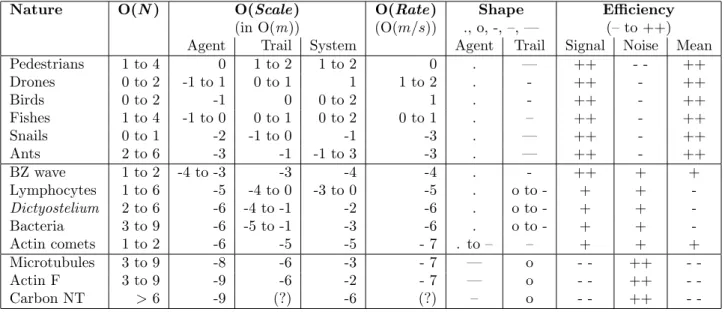
It is then evidence that the relative scale and intensity of the agent-trail related processes compared to that of the interfering processes is critical as well as the relative size of the agents compared to that of the trail signals. The table below (Table. 1) gives different examples of trail systems observed in nature or of artificial (hardware or simulated) ones.
Nature O(N ) O(Scale) O(Rate) Shape Efficiency
(in O(m)) (O(m/s)) ., o, -, –, — (– to ++)
Agent Trail System Agent Trail Signal Noise Mean
Pedestrians 1 to 4 0 1 to 2 1 to 2 0 . — ++ - - ++ Drones 0 to 2 -1 to 1 0 to 1 1 1 to 2 . - ++ - ++ Birds 0 to 2 -1 0 0 to 2 1 . - ++ - ++ Fishes 1 to 4 -1 to 0 0 to 1 0 to 2 0 to 1 . – ++ - ++ Snails 0 to 1 -2 -1 to 0 -1 -3 . — ++ - ++ Ants 2 to 6 -3 -1 -1 to 3 -3 . — ++ - ++ BZ wave 1 to 2 -4 to -3 -3 -4 -4 . - ++ + + Lymphocytes 1 to 6 -5 -4 to 0 -3 to 0 -5 . o to - + + -Dictyostelium 2 to 6 -6 -4 to -1 -2 -6 . o to - + + -Bacteria 3 to 9 -6 -5 to -1 -3 -6 . o to - + + -Actin comets 1 to 2 -6 -5 -5 - 7 . to – – + + + Microtubules 3 to 9 -8 -6 -3 - 7 — o - - ++ -Actin F 3 to 9 -9 -6 -2 - 7 — o - - ++ -Carbon NT > 6 -9 (?) -6 (?) – o - - ++
-Table 1: The table indicates the nature and the number of elements in a typical system. Semi-quantitative values (orders of magnitude expressed as exponents of ten) are given for their scales (agents, trails and the whole collective system) and the characteristic moving rates of the elements. Their shapes (agent and trail) can be assimilated as points ’.‘, round symmetric spread areas ’o‘ , or fibers weakly to strongly orientable (’-‘ to ’—‘)). An arbitrary notation between ’–‘ and ’++‘ characterizes the intensity of the trail signals. It is compared with the relative importance of the surrounding processes that interfere and perturb their behavior, thus giving an idea of the concurrence of the trail generation and trail degradation/spreading dynamics.
The table shows that very small and highly dynamic energy dependent elements behave potentially as trail systems : from the smaller to the bigger ones, actin filaments, microtubules, and actin comet systems. Due to the fact they are very small and numerous in a tiny volume of solution, and because they are fiber-shaped and consequently sensible to the action of weak external orienting fields like magnetic fields (18, 20, 21), they appear as excellent candidates for realizing programmable chemical processors based on this principle. Unfortunately, the table also shows that their scale is very close or the same to the microscopic level where intense molecular diffusion and transports of matter rapidly delete all useful information.
Actin comet systems such as bacteria-actin comets or those formed by latex coated beads are probably the most efficient trail systems at the microscopic scale because they produce highly concentrated, thin (order of 1 - 3 µm) and long (10 - 20 µm) trails, because the size of their agent (about 2 µm) is comparable to the width of the trails, and because on the contrary to single biological fibers, they are able to reorient rapidly in the preferential direction of the trails followed by reorganizing their fibrillar network. Movies of actin-beads or actin-bacteria comets realized by several teams perfectly show this behavior. Regrettably, the interactions between actin comet agents and trails still have not been studied. It would however be of great interest.
3
Modeling a single TS-agent
As mentioned in the introduction, in its deterministic form, our model uses the formalism of a Turing machine. Such an automaton is composed of a tape that contains informations and a head that reads the informations of the tape at its current position, that applies internal rules (or transitions) such as moving or changing its current state, and that can write new informations on the tape, all of this conditioned by the set of in-structions defined by the rules. Each Turing machine can be described as a sextuplet (Q, Σ, Γ, E, q0, F,#,),
on the tape (it does not include the blank character # that separate to values or instructions), Γ is the alphabet of the tape and includes Σ and #, q0 (q0 ∈ Q) is the initial internal state of the Turing machine,
F is the set of final states that can reach the Turing machine, and E is a finite set of transitions (or rules) written in the form of a quintuplet of symbols {c, r, n, w, m}. The transition parameters are the following : the current state of the Turing machine c, the current read state r, the new state of the Turing machine n, the new state to write on the tape w, and a move m. Such rules can also be noted c, r −→ n, w, m which means that if the Turing machine has the internal state c and reads r, its internal states changes to n, it replaces the symbol r by the symbol w in the tape and moves as indicated by m. All these symbols can be expressed into a unary, binary (or extended binary) or more compressed and symbolic (e.g. hexadecimal ...) codes. If it is of no importance for a Turing machine, we will see that the question of the encoding and the compression is really determining in the case of autonomous agents subject to stochasticity. For realizing any operation on values, the information tape has to contain at least these numerical or symbolic values, but can also contain the rules (sets of instructions encoded within the same tape) necessary for realizing this operation. In the latter case, the Turing machine is called universal. All values or instructions are delimited between specific separators (or blanks) also encoded in a certain format. In our case, we are not interested in universal Turing machines since we want our agent to be very distinct to the environment.
Here, in our model, we will not use a complicated formalism. We will limit the notation of the values in the tape (Σ) to the unary format where decimal number (d) 1 is the unary (u) 1, d2 = u11, d3 = u111 ..., so as the set of decimal values {0, 1, 2, 3...} corresponds to the unary values {0, 1, 11, 111...}. We differentiate the decimal number d0 (value u0) to the spacers used between these values by using the character star as a blank symbol (# = {∗}). The tapes and the sets of transitions are given separately (we are not in the case of universal Turing machines). The moves are elements of {S, L, R, P, T } for respectively Stay, go Left and go Right, Pause, and the stopping signal T (as Terminated), and are of length 0 (for stay, pause or stop) to 1 step relative to their current position. In the model, we make a distinction between Stay and Pause. Stay implies that the state of the agent has changed during this step so as the agent is not stopped. This move instruction can exist in both deterministic or stochastic systems. The move instruction Pause does not concern deterministic systems. Real systems can maintain themselves in a stationary state during a certain time (depending on their available amount of energy and on their energy consumption rate) when they are blocked. For example, we can immobilize an ant during a certain – short – time and it continues to live. Once freed, the ant can continue to move. Although it does not include the notion of energy, the instruction Pause mimics this possibility. In our model, only an stochastic change in the machine state, in the environment or of decision (transition) can unjam the agent. Another analogy with a living agent is when the agent faces to an impossibility to decide what to do because of an unknown situation. A certain time pass until the agent has an idea of how to do. This corresponds in our model to a stochastic change of the current used instruction.
The agents will always start at the extreme left of the tape and end their computation at the position of the last rightest symbol of the result with a stopping signal. Their internal states are represented by the symbols of the latin lowercase alphabet {a, b, c, ..., z}. All agents begin with the initial state a.
Bellow is shown, as an example, a simple Turing machine (highlighted in gray) that computes N plus one (here 3 + 1).
Transitions: (1) 0, a −→ 1, a, T ; (2) 1, a −→ 1, b, R ; (3) ∗, a −→ ∗, a, R ; (4) 1, b −→ 1, b, R ; (5) ∗, b −→ 1, b, T Tape before computation : * **111*** 3 + 1
Tape after computation : ***111 1 ** = 4
In our case, we want the agent to behave as a TS-agent would do. Our agent realizes a more inter-esting simple task, i.e. transporting values from one part of the tape to another. This mimics the manner ants transport food or materials from one part of their environment to another (for example, (26) show the aggregation dynamics of dead ants transported by living ants that release preferentially their loads when encountering an existing accumulation of ant corpses). The most simple TS-agent that simulates a deter-ministic – and very simplified – ant in a 1D environment can be written as described bellow :
Blanks and zeros are not equivalent. We aim to represent an environment that contains (1) or not (0) values that correspond to amounts of matter (e.g. food or dead ants), but we also want to include the notion of explored or unexplored environment. When explored by TS-agents the environment is modified and shows specific paths (trails) that other TS-agents or the same TS-agents that created these paths can use preferentially. In the following, the environment is first considered as unexplored and is filled by blank characters ∗ except in two areas that correspond to a source (e.g. the food) and a destination (e.g. the nest) that are heterogeneities in the environment susceptible to be sensed and modified by an agent. Both source and destination areas can initially contain quantities of matter equal or more than 0. The TS-agent is conceived to transport all the N symbols 1 from the right heap (source), if its initial value is more than 0, by copying them to the left heap (the destination which contains 0 (e.g empty nest) to M symbols 1 at the beginning). Firstly, the TS-agent is looking for a food source by traveling through its nest and then through
the unexplored area that separate the destination and the source areas. Then, when it finds some food, it comes back to the nest and let behind it a ’trail’ of 0. The character 0 represents here (in this very simplified model) both amount values equal to 0 and the presence of pheromones. Then, it adds the carried value to the heap and goes again to the food source, this time by ’following’ the traces of pheromones (succession of characters 0) between the two heaps. For doing that it needs the use of specific rules. At the end, the source disappears completely. This correspond to a calculus equivalent to N + M . Here N = 8 and M = 1. Of course much more simple models of Turing machines could do the same (i.e. transporting values from one heap to the other), but we aimed to be able to do a certain analogy with a trail system (with the notion of trail released by a TS-agent).
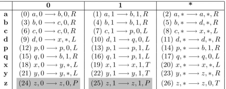
As described in table 2, the model contains 25 programmed transitions and 2 others – number 24 and 25 – (highlighted in gray) that where automatically added by the program so as to complete the table of relations between the TS-agent states and the environment values. The completion of the table is very important as is authorizes simulating stochastic systems. In such systems, . The two added instructions force the TS-agent to pause. As said before, only an accident let the TS-agent move again. Roughly, transitions 0-2 and 4-5 are used for reaching the left heap and crossing it, transitions 10-11 and 15-17 are used for realizing the first travel of 1 symbol 1 from the right to the left, transitions 3, 6-7 and 12-14 are used for transporting the N-1 symbols 1 from the right to the left, and finally the last transitions (8-9, 18-23 and 26) are used for reaching the left heap for the last time and finally stopping. The transitions that are characteristic to a trail system are those that imply the release and the use of a pheromone trail as a guiding rail, i.e. transitions 3, 6-10, 12, 17-18 and 21. 0 1 * a (0) a, 0 −→ b, 0, R (1) a, 1 −→ b, 1, R (2) a, ∗ −→ a, ∗, R b (3) b, 0 −→ c, 0, R (4) b, 1 −→ b, 1, R (5) b, ∗ −→ d, ∗, R c (6) c, 0 −→ c, 0, R (7) c, 1 −→ p, 0, L (8) c, ∗ −→ x, ∗, L d (9) d, 0 −→ x, ∗, L (10) d, 1 −→ q, 0, L (11) d, ∗ −→ d, ∗, R p (12) p, 0 −→ p, 0, L (13) p, 1 −→ p, 1, L (14) p, ∗ −→ b, 1, R q (15) q, 0 −→ b, 1, R (16) q, 1 −→ p, 1, L (17) q, ∗ −→ q, 0, L x (18) x, 0 −→ y, ∗, L (19) x, 1 −→ x, 1, T (20) x, ∗ −→ x, ∗, L y (21) y, 0 −→ y, ∗, L (22) y, 1 −→ y, 1, T (23) y, ∗ −→ z, ∗, R z (24) z, 0 −→ z, 0, P (25) z, 1 −→ z, 1, P (26) z, ∗ −→ z, 0, T
Table 2: Transitions. The table gives the possible actions of the TS-agent modelized here, depending on its current state (first column) and on the symbols read in the environment (first row). To a given TS-agent state and a symbol read each transition associates a new state, a symbol newly written at the current place of the TS-agent and a move.
3.1
Deterministic simulations
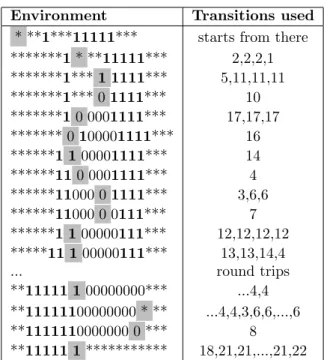
The principal steps of a deterministic simulation are given below in table 3. Is this simulation, the TS-agent transports 5 symbols 1 (at the right of the environment) to its nest (close to the left end of the environment) already containing a symbol 1.
Such a TS-agent behaves, in a simplified manner, as a deterministic foraging ant in a 1D environment (see fig. 2). In this example, if the right heap is absent, the deterministic TS-agent will never stop (and is invalid). The TS-agent would explore permanently its environment to the right until infinity. One could imagine by using different rules to place the food at the left and the nest to the right. In this case, if the nest was absent, it would be as if a unique dead ant or a very limited source of food was present in a box with a living deterministic one : the carrier ant would never release its load (until it dies in its turn). The only way for such a deterministic TS-agent to release the carried material is to include stochasticity in its perception of the environment, in its rules, or in the environment itself. Of course, more efficient rules could also be used that would ensure the deterministic TS-agent to stop such a set rules that would count the number of steps during when nothing has happened but our model is interesting in the sense that it is very simple and because its robustness is only due to the fact that there is no noise or errors and everything needs to be well planned before, until the presence of both a nest and a food source. Below is shown a complete simulation Of course, this deterministic automaton realize its task perfectly and will serve as a reference. Let us consider now the introduction of stochasticity in both the environment and the behavior of the TS-agent.
Environment Transitions used * **1***11111*** starts from there
*******1 * **11111*** 2,2,2,1 *******1*** 1 1111*** 5,11,11,11 *******1*** 0 1111*** 10 *******1 0 0001111*** 17,17,17 ******* 0 100001111*** 16 ******1 1 00001111*** 14 ******11 0 0001111*** 4 ******11000 0 1111*** 3,6,6 ******11000 0 0111*** 7 ******1 1 00000111*** 12,12,12,12 *****11 1 00000111*** 13,13,14,4 ... round trips **11111 1 00000000*** ...4,4 **11111100000000 * ** ...4,4,3,6,6,...,6 **1111110000000 0 *** 8 **11111 1 *********** 18,21,21,...,21,22
Table 3: Example of deterministic simulation. In the left column of the table, we show the principal steps of the evolution of the environment due to the action of the TS-agent. The position of the TS-agent is highlighted in gray. It becomes a TS-agent when it starts to release a trail of 0 (rules 10 and 17) on the return to its nest once it finds food (right heap of symbols 1), and when it uses it to come back from the nest (left heap of symbols 1) to the food. In the right column of the table, we give the respective transitions used for obtaining the environments at each step.
3.2
Imperfect TS-agents in a changing environment
In real life, stochasticity is everywhere but living systems spend a lot of energy to counter entropy and maintain coherent self-organized forms and behaviors. Every living agent exists in a given environment. Both can be sources of errors that can affect the behavior of agents. A living agent makes 4 different things in its life : the agent can sense its environment, the agent can modify the environment, it moves through the environment, and finally it possesses its internal life, as to say it can think, make decisions, dream, change its internal states, etc, all of this independently to the environment. Mistakes of the agents can appear at these 4 levels. Problems of attention or sensing are related to the sensitivity of agents to their environment, e.g. our hearing or the sensitivity of a chemotactic cell (density and quality of the membrane receptors). Difficulties in the persuasion, talking or writing (communication) are due to a limited intensity of the signals emitted by agents towards other agents through the environment, compared with the ambient noise already present in the environment. Here, we distinguish between the errors of moving and the errors of decision. An agent can choose to move somewhere, i.e. to the left, and finally does something else like moving back-wards or pausing. Stochastic changes of decision or, said differently, of use of behavioral rules always occur in our life when we feel uncertain about something to do before any choice of action (communicating or moving). Smaller living systems such as cells show most of the time coherent behaviors but sometimes, due to stochastic small molecular changes (e.g. a small excess or lack at one moment of a transcription factor in a cell compared to another very similar cell will cause a small difference of behavior between them during a certain time. In this example, the brain that makes decisions is the cell internal machinery), they don’t do what is expected. We are familiar to coherent behaviors of populations of cells, but when one look at all individual behaviors of each cells in the population, one find them not so coherent between each others.
In the environment, many events can also occur independently to living agents but all come down to transport of matter and transformation of matter. Transport of matter includes diffusion and flows but not the active transport of matter by living agents. Transformation of matter concerns chemical reactions, mu-tations, and disintegrations. All these phenomena are critical for the trails to be maintained. If weak trails are subject to a strong diffusion, the signal is rapidly diluted and the environment to become uniform again. On the contrary very intense trails produced by TS-agents in a noiseless environment will be maintained over a long time. In our model, the representation of both the environment and the level of functioning of TS-agents are microscopic. At this level, one can consider that errors, noise and transport penomena are rare events. Moreover, we consider distance matrices between the symbols of a given set (i.e. the set of rules, the set of moves, the set of TS-agent states, or the set of read symbols). Each distance value gives the relative proximity between two symbols (e.g. ’99’ is close to ’100’ but far from ’3’ as well as moving symbol
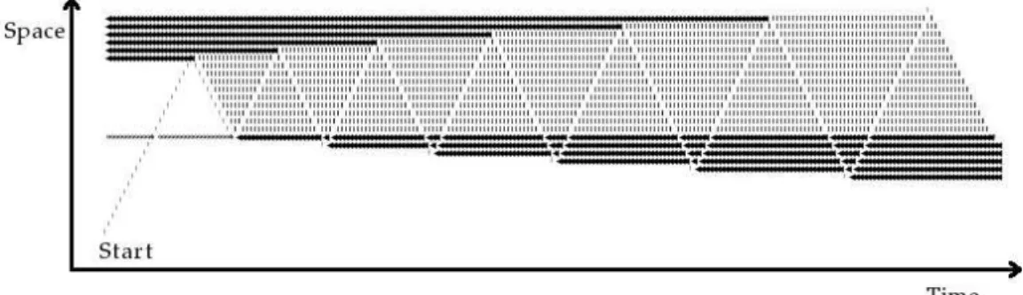
Figure 2: Trajectory of a 1D-ant. The TS-agent starts as indicated at the down left corner and moves vertically. The two heaps are shown in black: a big one (the food source which value = 6) at the top left corner and the smaller one (the nest which value = 0) below. They are separated initially by a blank space. Its trajectory during time corresponds to the zigzag that finishes to halt on the top of the nest. When moving, after it finds ’food’, it releases a trail that appears in gray between the two heaps. At the end, the trail is removed by the TS-agent and the environment contains only one heap which value = 6, i.e. the sum of the two heaps.
’L’, ’R’ and ’P’ are very close together, but far from the halting signal ’T’). Then every event, whatever its type, behaves as a microscopic diffusion event in our model since the errors or mutations are just stochastic jumps from one given value (e.g. a TS-agent state, a given move or an environment symbol) to another of the same set. These jumps are only authorized as imposed and limited by the distance matrices. In addition, as in diffusion phenomena anisotropy can also be applied to the diffusion phenomena in our sets of symbols so as to force the system to evolve in one direction. As an example, one can consider a set of integer symbols comprised between 0 and 100 that represent the local number of molecules in a small volume. Due to chemical events called disintegration or mutation, these molecules will be degraded into others that are not perceived by our TS-agent ; in other terms, for us, they disappear. Mutations events are then described as diffusion events of 1 step only from higher values to lower values of symbols.
Below is given the sequence of procedures followed during any simulation:
● Environmental events
– Calculate the mutations (Diffusion at a given location within the set of environment symbols) – Calculate the axial diffusion along the 1D environment
– Calculate the lateral diffusion between neighboring environments (in case of several parallel arrays of 1D environments)
● Individual action and events of the TS-agent
– Perception : the TS-agent reads the environment. A possible error occurs during reading : the TS-agent reads something else, close to the good value as defined by the matrix of environmental symbols.
– Decision : a rule is chosen given the environmental symbol read and the current state of the TS-agent. An error can occur that force the TS-agent to follow another transition close to the good one as indicated by the distance matrix of transitions. The state of the TS-agent takes a new value given by the transition that has been chosen.
– Communication : the TS-agent writes into the environment the symbol given by the transition that has been chosen before. A possible error occurs during writing : the TS-agent writes something else, close to the good value as defined by the matrix of environmental symbols.
– Moving : the TS-agent moves as described in the chosen rule. A possible error occurs during moving : the TS-agent moves in another direction or pauses or stops depending on the distance of the move states indicated by the matrix of move symbols.
At each time step, for one TS-agent, only one event of each type of event can occur. However, several events of mutation, and diffusion can occur in the environment during the same time because it is composed of several ’independent’ volumes. Then, at each time step, a Poisson distribution law is used to determine the number of diffusion events of each type (axial diffusion, lateral diffusion and mutations).
Because errors can cause the TS-agent move out of the limits of the first defined environment, the 1D environment can extend in the two directions ore we can decide that its geometry is toric. When the en-vironment extends, we generate a blank space and we fill it with the default symbols that characterize the basic level of the environment (full of molecules or empty, or undefined ...). During the simulation time many diffusion events and mutations occurred in the visible environment but many other should also have
occurred in the undefined regions that we create for the TS-agent to continue moving. Because of this, when we extend the environment in a direction, we add a certain number (typically 5 or 10) of spatial elements, we determine the number of each type of diffusion events that should have occurred during all the simulation and we generate them.
As illustrated by figure 3, where we applied a mutation rate λPoisson = 0.005 (it is a quite small
rate) on the environment with a strong anisotropy towards the smaller values (0 → 1 → ∗), some mutations occur and the trajectory of the TS-agent is punctuated by accidents. At the end, the result is not so different to the reference. Here, the resulting nest heap has the value 5 when the reference was 6. The execution of the simulations several thousand or million times will give an average result and its standard deviation. With these parameters, among 100000 simulations 90.2% had at least one error and we obtained an average result of 5.43 ± 1.76. Other comparisons could be made on other values such as the average Hamming distance between the final environments and the reference (here 0.092 ± 0.128), the computational time (number of steps) (here 220 ± 129 compared to the 225 steps of the reference), ... This constitutes a vector result that allows us measuring the efficiency of the considered trail system. This is a manner to quantify its robustness depending on its parameters.
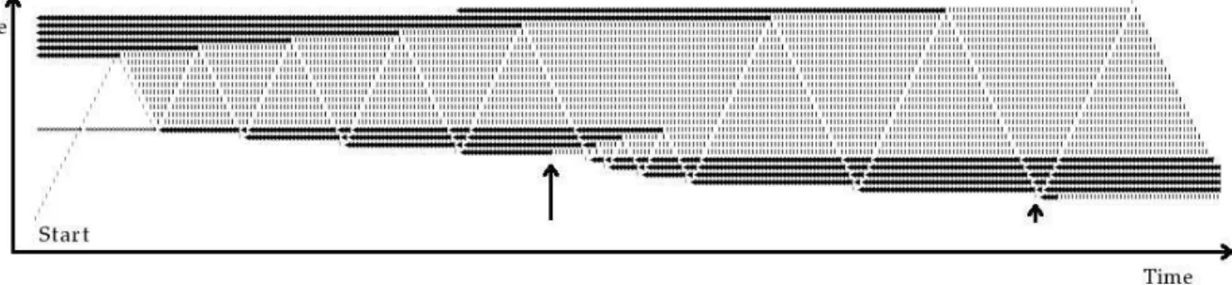
Figure 3: Trajectory of a 1D-ant in a changing environment. The simulations is identical to that described in figure 2 except that a mutation rate λPoisson = 0.003 is applied on the environment with a strong anisotropy towards the smaller values (0 → 1 → ∗). Only one mutation occurred as indicated by the arrow, and forced the TS-agent to follow a different trajectory during a certain time.
4
Increasing scales and degeneracy for robustness
For isolated TS-agents, in addition to the role of distance matrices that avoid dramatic changes when a perturbation occurs, two features ensure the robustness of TS-agent behaviors compared to a deterministic reference : the scale-depending accuracy of the agent in the perception of its environment, and the de-generacy of the values, internal states and rules in the system. First, we mentioned that in the present model, TS-agents have a sight distance over the environment of only one element. Of course, we could decide that our TS-agents could look at several elementary regions of the environment at the same time and that the environment effectively perceived is an average value or a maximum, or values superiors to a certain threshold. In our model, one can consider the case of a TS-agent looking at 3 contiguous elements of the environment centered on the central one. If its actions need at least one value different to ’0’ or ’*’ among the set of values read, the agent will be very robust in an environment where the trail signals degrade rapidly (conversions of ’1’ into ’0’ and of ’0’ into ’*’). The same phenomenon would have dramatic consequences on a TS-agent looking at only one element of space. The change of only one ’1’ into a ’0’ in that environment would change completely its computational trajectory. As evident they are, these remarks take sense when we think at biological systems such as cells that often perceive different regions of space at the same time due to a certain distribution of receptors on their surface. They are macroscopic agents that sense microscopic signals (individual molecules) with microscopic receptors. Microtubules on the contrary are microscopic agents that can only perceive very small regions which size are comparable to the dimensions of their sensing ends. In the first case (robust agent), the agent can ignore the fluctuation that exist at a scale level largely small than the agent itself; i.e. even if some of its receptors are not activated because of the local absence of molecules, a cell moving in a environment concentrated in activating molecules possess numerous other receptors that will perceive the signal. The cell feels globally concentrations instead of individual molecules and due to the integration of the whole concentration signal, the cell will adopt a certain behavior. On the contrary, when the size of agents is very limited compared to the size of the elements that compose the trail signal and to the trail itself, the agent will be very sensible to microscopic fluctuation.
Multivaluation on the symbols or values that describe the environment (e.g. ∗, 0, 1, 2, ... 106 ...) can
can contain this time more than one ’molecule’. The two environments compared in table 4 contain the same values but shown at two different zoom levels : a microscopical one at which the components are individualized (the environment contains 0 or 1 molecule in each element of space), whereas the elements of space of the more macroscopic one can contain up to 4 molecules. It can also be useful to represent envi-ronments that can contains several equivalent kinds of molecules that can be used by agents. An example is described in table 5. Of course, in the latter, the TS-agent has to know what to do when values up to 4 are
Microscopic view ... 0000 0011 1111 1011 1000 0000 ...
Macroscopic view ... 0 2 4 3 1 0 ...
Table 4: Scaling of the perception of environments. Both show the same but at two different zoom levels. Each macroscopic element of space corresponds to 4 microscopic elements.
encountered. This implies a degeneracy of their rules. For example, rule 7 of the model that corresponds for the agent to the action of picking a ’1’ and replacing it by a ’0’ – that means at the same time presence of pheromone and absence of food –, could be rewritten for a 6-valued environment (*, 0, 1, 2, 3, 4) as follows : Rule 7.1 : c, 1 −→ p, 0, L
Rule 7.2 : c, 2 −→ p, 1, L Rule 7.3 : c, 3 −→ p, 2, L Rule 7.4 : c, 4 −→ p, 3, L
Finally, another manner to introduce robustness is to multiply the number of redundant internal states (i.e. that are related to the same function). Such an increase of similar rules prevents the system from errors of decision or of fluctuations of the internal state.
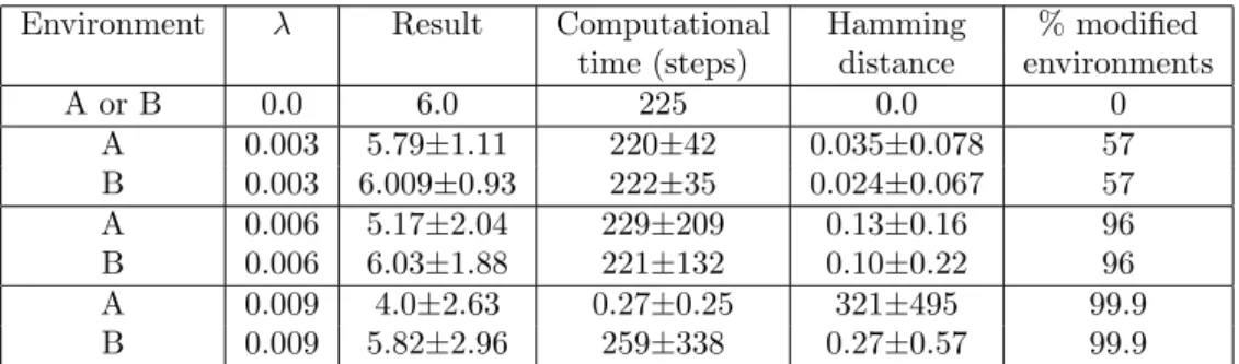
Environment λ Result Computational Hamming % modified
time (steps) distance environments
A or B 0.0 6.0 225 0.0 0 A 0.003 5.79±1.11 220±42 0.035±0.078 57 B 0.003 6.009±0.93 222±35 0.024±0.067 57 A 0.006 5.17±2.04 229±209 0.13±0.16 96 B 0.006 6.03±1.88 221±132 0.10±0.22 96 A 0.009 4.0±2.63 0.27±0.25 321±495 99.9 B 0.009 5.82±2.96 259±338 0.27±0.57 99.9
Table 5: Effect of redundancy in the environment. We defined two very similar environments A and B. Environment A is as previously defined in the article. Environment B contains 2 symbols (’1’ and ’—’) that are equivalent to symbol ’1’ and is initiated with symbols ’—’ instead of the ’1’ in environment A. The distance matrix for mutations is defined such as a mutation of ’—’ gives ’1’ that can give in its turn ’0’ due to another mutation. The rules of the corresponding agent are adapted so as the actions are equivalent when symbols ’1’ and ’—’ are encountered. Result data are given as a vector of 3 values : the resulting heap, the computational time, the Hamming distance between the resulting environment and its reference (λ = 0). They where obtained for each value of λ and for each environment by realizing 105
independent simulations. The average and standard deviations are given. We also indicate the percentage of modified environments among the 105
ones. Standard deviations are often large, but we still conserve well defined Gaussian distributions. Agent B is clearly more robust in its environment compared to agent A in environment A even if we only add a very low redundancy.
5
Populations of TS-agents
Until now, we focused on the microscopic behavior of individual TS-agents in their environment. Of course TS-agents become interesting when they participate to the collective behavior of a colony. TS-agents com-municate between each others via signals released to and get from their environment. In our model, this functionality is present. Diffusion can occur between neighboring 1D-environments. In real systems indeed, exchange of information helps maintaining a certain coherence of the whole system. This point is very well described in the recent article of Lizier et al (42). The question is to quantify the information transfer as a dependence of the future states of the receiving agent on the past states that were emitted by the source. As
said in that article, very logically, the predictive information transfer is the “average information contained in the source about the next state of the destination that was not already contained in the destination’s past.” This can be easily measured in our model of trail system by labeling with the ID label (unique identification number) of each agent, the environmental symbols that they manipulate. For example, a pheromone trail released by TS-agent N˚1 will be marked as ID-1 while that released by TS-agent N˚2 will be marked as ID-2. If TS-agent N˚1 uses the pheromones marked ID-2 (or reciprocally) it will be considered as an information transfer and scored. Then, from this individual measurements we obtain an average measure called ’transfer entropy’ that quantifies “the statistical coherence between systems evolving in time in a directional and dynamic manner”.
In real systems, such measurements are not always so easy to realize. First, it is difficult to know if for a given signal, a receiving agent has been able to effectively increase its information. Concerning human trails, the pedestrians can be asked on what they perceived and on how much they found useful the informations (e.g. cairns) available in the environment. For other systems, in particular small biological systems (cells, biological assemblies ...) fluorescent staining experiments could be realized in which groups of TS-agents (or individual ones) would be stained with a fluorophore of a first type (e.g. in green) and would emit trail signals of the same type, while other TS-agents would be marked by another sort of fluorophore (e.g. a red one). Matter exchanges could then be followed. As an example one could consider two actin comets one stained in red and the other in green. Both are constituted by actin monomers (red or green, depending on their origin). When disassembling, the red actin comet releases red stained actin monomers that can be assembled another time. If they are assembled into the green actin comet, an exchange of matter occurred between the red and the green comets. This means that the red monomers participated to the behavior of the green comet and modified it. Realistic simulations of real systems are also a good way to evaluate such transfer entropy by following matter exchanges (simulations shown in fig. 4 aims to follow the individual trajectory of tubulin-GDP proteins).
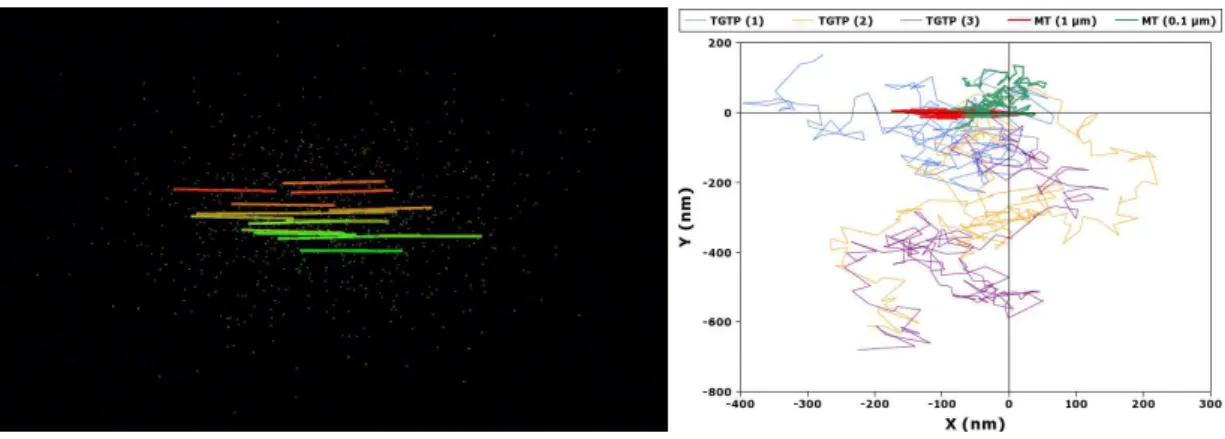
Figure 4: (left) On the left side, we show a simulation of microtubule disassembly, where 15 microtubules are marked by different colors. The tubulin-GDP they release is marked by the same color. This allows following the exchanges of matter between microtubules. (right) A detail is shown on the right side of the figure : A transversal projection of the 3D trajectory of 2 microtubules and 3 tubulin molecules is followed. As tubulin is quasi-spheric, its diffusion is isotropic. On the contrary, microtubules are rod like shaped and, depending on their size, their rotational and translational diffusion along their 3 axes is not equivalent, that way resulting in an anisotropic diffusion.
The study of the communication between trail systems and of how its efficiency is crucial for the TS-agents to self-organize locally, needs a separate paper. Nevertheless, we would like to mention two important points : the first one concerns the robustness of the process and its relations with the level of description of the environment, the second one the synchronism of agents.
● (A) As mentioned in the previous section, the same environment can be described at different scale
levels. At the most microscopical one, each event of mutation or transport of matter appears clearly as a dramatic change. If our TS-agents work at such microscopic levels, then they will be very sensible to such changes. On the contrary, if their sensing surface is extended to a more macroscopic area, small changes have no consequences because they are compensated by the presence of numerous other ’normal’ events. Another manner to increase the robustness of the individual behaviors of agents (and to represent large views of the environment in a limited number of areas) is to use multivaluation of the symbols that describe the environment and the degeneracy of the transitions in whose these symbols will be involved. For example, one can decide that our TS-agent covers a surface that can contain up to 1000 molecules and that our TS-agent has three different behaviors depending on two thresholds
: less than 10 molecules, more than 10 and less than 100 (a zone of transition), and more than 100 molecules. We will use a representation of the environment in which each subvolume contains up to 1000 values (or symbols) but our TS-agent will need only 3 rules (and not 1000) to know what to do in such an environment. Before, we considered only one TS-agent moving in its own 1D environment. The addition of lateral diffusion in our model (between the neighboring 1D environments) can cause dramatic accidents in the behavior of the agents, depending notably on that point.
● (B) The other criterion that will affect the local robustness of individual behaviors and the local
information transfer is of temporal nature. The synchronism of the functioning of the agents (and the correlation of their activities), or on the contrary their asynchrony will affect considerably the information transfer during all their lifetime. If the agents are synchronous, like perfect robots, no information transfer will occur until the machines come back on their own steps. By lateral diffusion, the environment modified by TS-agent N˚1 can diffuse to environment N˚2 (and reciprocally), but even if it was the case, TS-agent N˚2 would be yet at its next state and would move before sensing the change in environment N˚2 (and reciprocally for TS-agent N˚1 ). If they come back on their own trajectory, they will be able, that time, to sense the changes that occurred in their past. Such ’machines’ are not very interesting because they do not communicate easily (and locally in a spatio-temporal sense). Moreover, agents in real systems never work synchronously, even when we think they do. There is always one agent in the populations that is more advanced in its – computational – trajectory and in its decisions than the others. One of our students tall us a very good example, that happened to him, which illustrate exactly that point : he was walking with a friend in our city of Grenoble. Both aimed to go to a precise point in the town, but none of them knew where it was, and both thought that the other knew. So they walked while talking to each other of other things, each of them being sure that the other was going in the good direction. They walked during at least half and hour before asking them the question of yes or no the other knew. In a very theoretical system, if these two agents were synchronous, this situation could never occur. In reality, although they looked to walk together in a synchronous manner, their trajectory was decided because at each time, the decision to walk forward in a specific direction was made before by one of them, and the other followed this one. In our model, the individual action steps of the TS-agents are clocked (1 action per 1 time step), but for allowing asynchrony, we introduce random waiting steps. In consequence, if a population of individual was realizing the computation showed in figs. 2 & 3, with several environments linked together by a certain relation of neighborhood, the most advanced TS-agent (in its own environment) would modify its environment and this should affect the behavior of the late ones, especially if they are not robust to such changes (see point A).
6
Programming a bioprocessor whom fine architecture is made
of trail systems self-organized structures
As in neural networks, ’programming’ means ’learning’ in such systems.
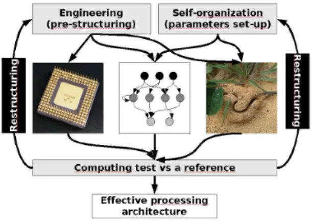
The conception of classical electronic-based computers took several dozen years to physicists and engi-neers. They started from very simple circuits that they tried to assemble logically so as to realized controlled calculii. They do not based their conceptions on any theoretical concepts such as Turing machines (a very interesting and puzzling history of the birth of computing machines was given by Burks (43, 44). After that, a kind of evolutionary process occurred and is still active where engineers try new architectures and complexifications that are then tested successively by them, by benchmarkers and by the consumers (fig. 5 left). There are two types of selection processes : one is purely functional and the other is related to the current preferences of a society in terms of technology. Only the functional architectures persist, but among them, only the most adapted to the needs and preferences of the consuming society survive. Our electronic processors must be able to compute and they must be able to be programmed easily and used by consumers or programmers. That coupling between all protagonists and the process of selection is very long.