Global and regional drivers of accelerating CO2 emissions

HAL Id: hal-02888539

https://hal.archives-ouvertes.fr/hal-02888539

Submitted on 7 Apr 2021

HAL is a multi-disciplinary open access

archive for the deposit and dissemination of

sci-entific research documents, whether they are

pub-lished or not. The documents may come from

teaching and research institutions in France or

abroad, or from public or private research centers.

L’archive ouverte pluridisciplinaire HAL, est

destinée au dépôt et à la diffusion de documents

scientifiques de niveau recherche, publiés ou non,

émanant des établissements d’enseignement et de

recherche français ou étrangers, des laboratoires

publics ou privés.

Global and regional drivers of accelerating CO2

emissions

M. Raupach, G. Marland, P. Ciais, C. Le Quéré, J. Canadell, G. Klepper, C.

Field

To cite this version:

M. Raupach, G. Marland, P. Ciais, C. Le Quéré, J. Canadell, et al.. Global and regional drivers of

accelerating CO2 emissions. Proceedings of the National Academy of Sciences of the United States of

America , National Academy of Sciences, 2007, 104 (24), pp.10288-10293. �10.1073/pnas.0700609104�.

�hal-02888539�

Global and regional drivers of accelerating

CO

₂

emissions

Michael R. Raupach*†_{, Gregg Marland}‡_{, Philippe Ciais}§_{, Corinne Le Que´re´}¶㥋_{, Josep G. Canadell*, Gernot Klepper**,}

and Christopher B. Field††

*Global Carbon Project, Commonwealth Scientific and Industrial Research Organisation, Marine and Atmospheric Research, Canberra, ACT 2601, Australia;‡_{Carbon Dioxide Information Analysis Center, Oak Ridge National Laboratory, Oak Ridge, TN 37831;}§_{Commissariat a` l’Energie}

Atomique, Laboratorie des Sciences du Climat et de l’Environnement, 91191 Gif sur Yvette, France;¶_{School of Environment Sciences, University of East} Anglia, Norwich NR4 7TJ United Kingdom;㛳British Antarctic Survey, Cambridge, CB3 OET, United Kingdom; **Kiel Institute for the World Economy, D- 24105 Kiel, Germany; and††_{Carnegie Institution of Washington, Department of Global Ecology, Stanford, CA 94305}

Edited by William C. Clark, Harvard University, Cambridge, MA, and approved April 17, 2007 (received for review January 23, 2007)

CO2emissions from fossil-fuel burning and industrial processes

have been accelerating at a global scale, with their growth rate

increasing from 1.1% yⴚ1for 1990 –1999 to >3% yⴚ1for 2000 –

2004. The emissions growth rate since 2000 was greater than for the most fossil-fuel intensive of the Intergovernmental Panel on Climate Change emissions scenarios developed in the late 1990s. Global emissions growth since 2000 was driven by a cessation or reversal of earlier declining trends in the energy intensity of gross domestic product (GDP) (energy/GDP) and the carbon intensity of energy (emissions/energy), coupled with continuing increases in population and per-capita GDP. Nearly constant or slightly increas-ing trends in the carbon intensity of energy have been recently observed in both developed and developing regions. No region is decarbonizing its energy supply. The growth rate in emissions is strongest in rapidly developing economies, particularly China. Together, the developing and least-developed economies (forming 80% of the world’s population) accounted for 73% of global emissions growth in 2004 but only 41% of global emissions and only 23% of global cumulative emissions since the mid-18th cen-tury. The results have implications for global equity.

carbon intensity of economy兩 carbon intensity of energy 兩 emissions scenarios兩 fossil fuels 兩 Kaya identity

A

tmospheric CO2presently contributes⬇63% of the gaseous

radiative forcing responsible for anthropogenic climate change (1). The mean global atmospheric CO2concentration has

increased from 280 ppm in the 1700s to 380 ppm in 2005, at a progressively faster rate each decade (2, 3).‡‡ _{This growth is}

governed by the global budget of atmospheric CO2(4), which

includes two major anthropogenic forcing fluxes: (i) CO2

emis-sions from fossil-fuel combustion and industrial processes and (ii) the CO2flux from land-use change, mainly land clearing. A

survey of trends in the atmospheric CO2budget (3) shows these

two fluxes were, respectively, 7.9 gigatonnes of carbon (GtC) y⫺1 and 1.5 GtC y⫺1in 2005 with the former growing rapidly over recent years, and the latter remaining nearly steady.

This paper is focused on CO2 emissions from fossil-fuel

combustion and industrial processes, the dominant anthropo-genic forcing flux. We undertake a regionalized analysis of trends in emissions and their demographic, economic, and technological drivers, using the Kaya identity (defined below) and annual time-series data on national emissions, population, energy consumption, and gross domestic product (GDP). Un-derstanding the observed magnitudes and patterns of the factors influencing global CO2 emissions is a prerequisite for the

prediction of future climate and earth system changes and for human governance of climate change and the earth system. Although the needs for both understanding and governance have been emerging for decades (as demonstrated by the United Nations Framework Convention on Climate Change in 1992 and the Kyoto Protocol in 1997), it is now becoming widely perceived that climate change is an urgent challenge requiring globally

concerted action, that a broad portfolio of mitigation measures is required (5, 6), and that mitigation is not only feasible but highly desirable on economic as well as social and ecological grounds (7).

The global CO2emission flux from fossil fuel combustion and

industrial processes (F) includes contributions from seven sources: national-level combustion of solid, liquid, and gaseous fuels; flaring of gas from wells and industrial processes; cement production; oxidation of nonfuel hydrocarbons; and fuel from ‘‘international bunkers’’ used for shipping and air transport (separated because it is often not included in national invento-ries). Hence

F⫽ FSolid

⬇35%⫹ FLiquid⬇36%⫹ F⬇20%Gas ⫹ FFlare⬍1%

⫹ FCement

⬇3% ,⫹ FNonFuelHC⬍1% ⫹ FBunkers⬇4% ,

[1]

where the fractional contribution of each source to the total F for 2000–2004 is indicated.

The Kaya identity§§_{(8, 9) expresses the global F as a product}

of four driving factors:

F⫽ P

冉

G P

冊冉

E G

冊冉

F E

冊

⫽ Pgef, [2]

where P is global population, G is world GDP or gross world product, E is global primary energy consumption, g⫽ G/P is the per-capita world GDP, e⫽ E/G is the energy intensity of world GDP, and f⫽ F/E is the carbon intensity of energy. Upper- and lowercase symbols distinguish extensive and intensive variables,

Author contributions: M.R.R., P.C., C.L.Q., J.G.C., and C.B.F. designed research; M.R.R., G.M., P.C., and J.G.C. performed research; M.R.R., G.M., P.C., and G.K. analyzed data; and M.R.R., G.M., G.K., and C.B.F. wrote the paper.

The authors declare no conflict of interest. This article is a PNAS Direct Submission.

Freely available online through the PNAS open access option.

Abbreviations: GDP, gross domestic product; MER, market exchange rate; PPP, purchasing power parity; IPCC, Intergovernmental Panel on Climate Change; EU, European Union; FSU, Former Soviet Union; D1, developed countries; D2, developing countries; D3, least-developed countries; CDIAC, U.S. Department of Energy Carbon Dioxide Information and Analysis Center; EIA, U.S. Department of Energy Energy Information Administration. †_{To whom correspondence should be addressed. E-mail: michael.raupach@csiro.au.} ‡‡_{CO2data are available at www.cmdl.noaa.gov/gmd/ccgg/trends.}

§§_{Yamaji, K., Matsuhashi, R., Nagata, Y., Kaya, Y., An Integrated System for CO} 2/Energy/

GNP Analysis: Case Studies on Economic Measures for CO2Reduction in Japan. Workshop

on CO2Reduction and Removal: Measures for the Next Century, March 19, 1991, International Institute for Applied Systems Analysis, Laxenburg, Austria.

This article contains supporting information online atwww.pnas.org/cgi/content/full/ 0700609104/DCI.

respectively. Combining e and f into the carbon intensity of GDP (h⫽ F/G ⫽ ef), the Kaya identity can also be written as

F⫽ P

冉

G P

冊冉

F

G

冊

⫽ Pgh. [3]

Defining the proportional growth rate of a quantity X(t) as

r(X) ⫽ X⫺1dX/dt (with units [time]⫺1), the counterpart of the Kaya identity for proportional growth rates is

r共F兲 ⫽ r共P兲 ⫹ r共 g兲 ⫹ r共e兲 ⫹ r共 f 兲 [4]

⫽ r共P兲 ⫹ r共 g兲 ⫹ r共h兲, which is an exact, not linearized, result.

The world can be disaggregated into regions (distinguished by a subscript i) with emission Fi, population Pi, GDP Gi, energy consumption Ei, and regional intensities gi⫽ Gi/Pi, ei⫽ Ei/Gi, fi⫽

Fi/Ei, and hi⫽ Fi/Gi⫽ eifi. Writing a Kaya identity for each region, the global emission F can be expressed by summation over regions as: F⫽

冘

i Fi⫽

冘

i Pigieifi⫽

冘

i Pigihi, [5]

and regional contributions to the proportional growth rate in global emissions, r(F), are

r共F兲 ⫽

冘

i

冉

Fi

F

冊

r共Fi兲. [6]

This analysis uses nine noncontiguous regions that span the globe and cluster nations by their emissions and economic profiles. The regions comprise four individual nations (U.S., China, Japan, and India, identified separately because of their significance as emitters); the European Union (EU); the nations of the Former Soviet Union (FSU); and three regions spanning the rest of the world, consisting respectively of developed (D1), developing (D2), and least-developed (D3) countries, excluding countries in other regions.

GDP is defined and measured by using either market exchange rates (MER) or purchasing power parity (PPP), respectively de-noted as GMand GP. The PPP definition gives more weight to developing economies. Consequently, wealth disparities are greater when measured by GMthan GP, and the growth rate of GPis greater than that of GM[supporting information (SI) Fig. 6].

Our measure of Eiis ‘‘commercial’’ primary energy, including

(i) fossil fuels, (ii) nuclear, and (iii) renewables (hydro, solar, wind, geothermal, and biomass) when used to generate electric-ity. Total primary energy additionally includes (iv) other energy from renewables, mainly as heat from biomass. Contribution iv

can be large in developing regions, but it is not included in Ei

except in the U.S., where it makes a small (⬍4%) contribution (SI Text, Primary Energy).

Results

Global Emissions. A sharp acceleration in global emissions oc-curred in the early 2000s (Fig. 1 Lower). This trend is evident in two data sets (Materials and Methods): from U.S. Department of Energy Energy Information Administration (EIA) data, the

proportional growth rate in global emissions [r(F)⫽ (1/F)dF/dt]

was 1.1% y⫺1 for the period 1990–1999 inclusive, whereas for

2000–2004, the same growth rate was 3.2%. From U.S. Depart-ment of Energy Carbon Dioxide Information and Analysis

Center (CDIAC) data, growth rates were 1.0% y⫺1through the

1990s and 3.3% y⫺1for 2000–2005. The small difference arises

mainly from differences in estimated emissions from China for 1996–2002 (Materials and Methods).

Fig. 1 compares observed global emissions (including all terms in Eq. 1) with six Intergovernmental Panel on Climate Change (IPCC) emissions scenarios (8) and also with stabilization tra-jectories describing emissions pathways for stabilization of

at-mospheric CO2at 450 and 650 ppm (10–12). Observed emissions

were at the upper edge of the envelope of IPCC emissions scenarios. The actual emissions trajectory since 2000 was close to the highest-emission scenario in the envelope, A1FI. More importantly, the emissions growth rate since 2000 exceeded that for the A1FI scenario. Emissions since 2000 were also far above the mean stabilization trajectories for both 450 and 650 ppm.

A breakdown of emissions among sources shows that solid,

liquid, and gas fuels contributed (for 2000–2004)⬇35%, 36%,

and 20%, respectively, to global emissions (Eq. 1). However, this distribution varied strongly among regions: solid (mainly coal) fuels made up a larger and more rapidly growing share of

1990 1995 2000 2005 2010 CO 2 Emissions ( G tC y -1 ) 5 6 7 8 9 10

Actual emissions: CDIAC Actual emissions: EIA 450ppm stabilization 650ppm stabilization A1FI A1B A1T A2 B1 B2 1850 1900 1950 2000 2050 2100 CO 2 E m issio n s (GtC y -1 ) 0 5 10 15 20 25 30

Actual emissions: CDIAC 450ppm stabilization 650ppm stabilization A1FI A1B A1T A2 B1 B2

Fig. 1. Observed global CO2emissions including all terms in Eq. 1, from both

the EIA (1980 –2004) and global CDIAC (1751–2005) data, compared with emissions scenarios (8) and stabilization trajectories (10 –12). EIA emissions data are normalized to same mean as CDIAC data for 1990 –1999, to account for omission of FCementin EIA data (see Materials and Methods). The 2004 and 2005 points in the CDIAC data set are provisional. The six IPCC scenarios (8) are spline fits to projections (initialized with observations for 1990) of possible future emissions for four scenario families, A1, A2, B1, and B2, which empha-size globalized vs. regionalized development on the A,B axis and economic growth vs. environmental stewardship on the 1,2 axis. Three variants of the A1 (globalized, economically oriented) scenario lead to different emissions tra-jectories: A1FI (intensive dependence on fossil fuels), A1T (alternative tech-nologies largely replace fossil fuels), and A1B (balanced energy supply be-tween fossil fuels and alternatives). The stabilization trajectories are spline fits approximating the average from two models (11, 12), which give similar results. They include uncertainty because the emissions pathway to a given stabilization target is not unique.

Raupach et al. PNAS 兩 June 12, 2007 兩 vol. 104 兩 no. 24 兩 10289

SUSTAINABILITY

emissions in developing regions (the sum of China, India, D2, and D3) than in developed regions (U.S., EU, Japan, and D1), and the FSU region had a much stronger reliance on gas than the world average (SI Fig. 7).

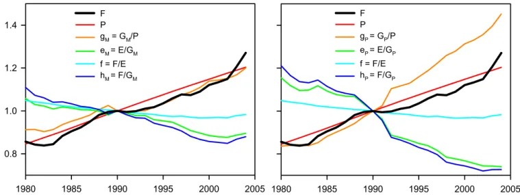
To diagnose drivers of trends in global emissions, Fig. 2 superimposes time series for 1980–2004 of the Kaya factors F, P,

g, e, f, and h⫽ ef (Eqs. 2 and 3). Fig. 2 Left and Right, respectively,

use the MER and PPP forms of GDP (GMand GP) to calculate

intensities. All quantities are normalized to 1 in the year 1990 to show the relative contributions of changes in Kaya factors to changes in emissions. Table 1 gives recent (2004) values without normalization.

In Fig. 2 Left (MER-based), the Kaya identity is F⫽ PgMeMf⫽

PgMhM(with gM ⫽ GM/P, eM⫽ E/GM, and hM⫽ F/GM). The

increase in the growth rate of F after 2000 is clear. Before 2000,

F increased as a result of increases in both P and gMat roughly

equal rates, offset by a decrease in eM, with f declining very

slowly. Therefore, hM⫽ eMf declined slightly more quickly than

eM. After 2000, the increases in P and gMcontinued at about their

pre-2000 rates, but eM and f (and therefore hM) ceased to

decrease, leading to a substantial increase in the growth rate of

F. In fact, both eMand f have increased since 2002. Similar trends

are evident in Fig. 2 Right (PPP-based), using the Kaya identity

F⫽ PgPePf⫽ PgPhP,(with gP⫽ GP/P, eP⫽ E/GP, and hP⫽ F/GP).

The long-term (since 1980) rate of increase of gPand the rates

of decrease of ePand hPwere all larger than for their

counter-parts gM, eM, and hM, associated with the higher global growth

rate of GPthan of GM(SI Fig. 6). There was a change in the

trajectory of ePafter 2000, similar to that for eMbut

superim-posed on a larger long-term rate of decrease. Hence, Fig. 2 Left and Right both identify the driver of the increase in the growth rate of global emissions after 2000 as a combination of reduc-tions or reversals in long-term decreasing trends in the global carbon intensity of energy ( f ) and energy intensity of GDP (e). Regional Emissions.The regional distribution of emissions (Fig. 3) is similar to that of (commercial) primary energy consumption

(Ei) but very different from that of population (Pi), with Fiand

Eiweighted toward developed regions and Pitoward developing

regions. Drivers of regional emissions are shown in Fig. 4 by plotting the normalized factors in the nine regional Kaya iden-tities, using GDP (PPP). Equivalent plots with GDP (MER) are nearly identical (SI Fig. 8).

In the developed regions (U.S., Europe, Japan, and D1), Fi

increased from 1980 to 2004 as a result of relatively rapid

growth in mean income (gi) and slow growth in population (Pi),

offset in most regions by decreases in the energy intensity of

GDP (ei). Declines in eiindicate a progressive decoupling in most

developed regions between energy use and GDP growth. The

carbon intensity of energy ( fi) remained nearly steady.

1980 1985 1990 1995 2000 2005 0.8 1.0 1.2 1.4 F P gM = GM/P eM= E/GM f = F/E hM= F/GM 1980 1985 1990 1995 2000 2005 F P gP= GP/P e_P= E/G_P f = F/E hP= F/GP

Fig. 2. Factors in the Kaya identity, F⫽ Pgef ⫽ Pgh, as global averages. All quantities are normalized to 1 at 1990. Intensities are calculated by using GM(Left)

and GP(Right). In both Left and Right, the black line (F) is the product of the red (P), orange (g), green (e), and light blue ( f) lines (Eq. 2) or equivalently of the

red (P), orange (g), and dark blue (h) lines (Eq. 3). Because h⫽ ef, the dark blue line is the product of the green and light blue lines. Sources are as in Table 1.

Table 1. Values of extensive and intensive variables in 2004 Fi,

MtC/y

Pi,

million Ei, EJ/y

GMi,

G$/y GPi, G$/y

gPi⫽ GPi/Pi, k$/y ePi⫽ Ei/GPi, MJ/$ fi⫽ Fi/Ei, gC/MJ hPi⫽ Fi/GPi, gC/$ Fi/Pi, tC/y Ei/Pi, kW U.S. 1,617 295 95.4 9,768 7,453 25.23 12.80 16.95 217.0 5.47 10.24 EU 1,119 437 70.8 10,479 7,623 17.45 9.29 15.81 146.8 2.56 5.14 Japan 344 128 21.4 4,036 2,412 18.85 8.89 16.05 142.7 2.69 5.31 D1 578 150 37.3 3,283 2,553 17.06 14.63 15.47 226.3 3.86 7.91 FSU 696 285 42.8 726 1,423 4.99 30.08 16.25 488.7 2.44 4.76 China 1,306 1,293 57.5 1,734 5,518 4.27 10.43 22.70 236.6 1.01 1.41 India 304 1,087 14.6 777 2,130 1.96 6.86 20.77 142.5 0.28 0.43 D2 1,375 2,020 80.9 4,280 7,044 3.49 11.49 16.99 195.2 0.68 1.27 D3 37 656 2.2 255 609 0.93 3.66 16.78 61.4 0.06 0.11 World 7,376 6,351 423.1 35,338 36,765 5.79 11.51 17.43 200.6 1.16 2.11

In the FSU, emissions decreased through the 1990s because of the fall in economic activity after the collapse of the Soviet Union. Incomes (gi) decreased in parallel with emissions (Fi), and a shift toward resource-based economic activities led to an increase in eiand hi. In the late 1990s, incomes started to rise again, but increases in emissions were slowed by more efficient use of energy from 2000 on, due to higher prices and shortages because of increasing exports.

In China, girose rapidly and Pislowly over the whole period 1980–2004. Progressive decoupling of income growth from energy

consumption (declining ei) was achieved up to ⬇2002, through improvements in energy efficiency during the transition to a market based economy. Since the early 2000s, there has been a recent rapid growth in emissions, associated with very high growth rates in incomes (gi) and a reversal of earlier declines in ei.

In other developing regions (India, D2, and D3), increases in

Fiwere driven by a combination of increases in Piand gi, with no strong trends in eior fi. Growth in emissions (Fi) exceeded growth in income (gi). Unlike China and the developed countries, strong technological improvements in energy efficiency have not yet occurred in these regions, with the exception of India over the last few years where eideclined.

Differences in intensities across regions are both large (Table 1) and persistent in time. There are enormous differences in income (gi⫽ Gi/Pi), the variation being smaller (although still large) for gPi than for gMi. The energy intensity and carbon intensity of GDP (ei ⫽ Ei/Gi and hi ⫽ Fi/Gi ⫽ eifi) vary significantly between regions, although less than for income (gi). The carbon intensity of energy ( fi⫽ Fi/Ei) varies much less than other intensities: for most regions, it is between 15 and 20 grams of carbon per megajoule (gC/MJ), although for China and India it is somewhat higher, ⬎20 gC/MJ. In time, fihas decreased slowly from 1980 to⬇2000 as a global average (Fig. 2) and in most regions (Fig. 4). This indicates that the commercial energy supply mix has changed only slowly, even on a regional level. The global average f has increased slightly since 2002.

The regional per-capita emissions Fi/Pi⫽ gihiand per-capita primary energy consumption Ei/Pi⫽ gieiare important indicators of global equity. Both quantities vary greatly across regions but much less in time (Table 1 andSI Fig. 9). The interregion range,

a factor of⬇50, extends from the U.S. (for which both quantities

are⬇5 times the global average) to the D3 region (for which they

CO₂ Emissions (MtC y-1) 1980 1982 19841986 1988 1990199219941996199 8 200 0 200 2 200 4 0 1000 2000 3000 4000 5000 6000 7000 8000 D3 D2 FSU D1 China India EU Japan USA

Fig. 3. Fossil-fuel CO2emissions (MtC y⫺1), for nine regions. Data source is

EIA.

FSU

USA

0.5 1.0 1.5 2.0

EU

F P g_P = GP/P e_P = E/GP f = F/E h P = F/GP

Japan

D1

0.5 1.0 1.5 2.0

China

India

1980 1985 1990 1995 2000 0.5 1.0 1.5 2.0

D2

1980 1985 1990 1995 2000

D3

1980 1985 1990 1995 2000 2005

Fig. 4. Factors in the Kaya identity, F⫽ Pgef ⫽ Pgh, for nine regions. All quantities are normalized to 1 at 1990. Intensities are calculated with GPi(PPP). For

FSU, normalizing GPiin 1990 was back-extrapolated. Other details are as for Fig. 2.

Raupach et al. PNAS 兩 June 12, 2007 兩 vol. 104 兩 no. 24 兩 10291

SUSTAINABILITY

are ⬇1/10 of the global average). From 1980 to 1999, global average per-capita emissions (F/P⫽ gh) and per-capita primary energy consumption (E/P⫽ ge) were both nearly steady at ⬇1.1 tC/y per person and 2 kW per person, respectively, but F/P rose by 8% and E/P by 7% over the 5 years 2000–2004.

Temporal Perspectives.In the period 2000–2004, developing

coun-tries had a greater share of emissions growth than of emissions themselves (Fig. 3). Here we extend this observation by consid-ering cumulative emissions throughout the industrial era (taken to start in 1751). The global cumulative fossil-fuel emission C(t) (in gigatonnes of carbon) is defined as the time integral of the global emission flux F(t) from 1751 to t. Regional cumulative emissions Ci(t) are defined similarly.

Fig. 5 compares the relative contributions in 2004 of the nine regions to the global cumulative emission C(t), the emission flux

F(t) [the first derivative of C(t)], the emissions growth rate [the

second derivative of C(t)], and population. The measure of regional emissions growth used here is the weighted propor-tional growth rate (Fi/F)r(Fi), which shows the contribution of each region to the global r(F) (Eq. 6). In 2004, the developed regions contributed most to cumulative emissions and least to emissions growth, and vice versa for developing regions. China in 2004 had a larger than pro-rata share (on a population basis) of the emissions growth but still a smaller than pro-rata share of actual emissions and a very small share of cumulative emissions. India and the D2 and D3 regions had smaller than pro-rata shares of emissions measures on all time scales (growth, actual emissions, and cumulative emissions).

Discussion

CO2emissions need to be considered in the context of the whole

carbon cycle. Of the total cumulative anthropogenic CO2

emis-sion from both fossil fuels and land use change, less than half remains in the atmosphere, the rest having been taken up by land and ocean sinks (ref. 4;SI Text, The Global Carbon Cycle). For the recent period 2000–2005, the fraction of total anthropogenic

CO2 emissions remaining in the atmosphere (the airborne

fraction) was 0.48. This fraction has increased slowly with time (J. G. Canadell, C.L.Q., M.R.R., C.B.F., E. T. Buitenhaus, et al., unpublished data), implying a slight weakening of sinks relative to emissions. However, the dominant factor accounting for the

recent rapid growth in atmospheric CO2(⬎2 ppm y⫺1) is high

and rising emissions, mostly from fossil fuels.

The strong global fossil-fuel emissions growth since 2000 was driven not only by long-term increases in population (P) and per-capita global GDP (g) but also by a cessation or reversal of earlier declining trends in the energy intensity of GDP (e) and the carbon intensity of energy ( f ). In particular, steady or slightly increasing recent trends in f occurred in both developed and developing regions. In this sense, no region is decarbonizing its energy supply.

Continuous decreases in both e and f (and therefore in carbon

intensity of GDP, h⫽ ef) are postulated in all IPCC emissions

scenarios to 2100 (8), so that the predicted rate of global emissions growth is less than the economic growth rate. Without these postulated decreases, predicted emissions over the coming century would be up to several times greater than those from current emissions scenarios (13). In the unfolding reality since 2000, the global average f has actually increased, and there has not been a compensating faster decrease in e. Consequently, there has been a cessation of the earlier declining trend in h. This has meant that even the more fossil-fuel-intensive IPCC scenar-ios underestimated actual emissions growth during this period. The recent growth rate in emissions was strongest in rapidly developing economies, particularly China, because of very strong

economic growth (gi) coupled with post-2000 increases in ei, fi,

and therefore hi ⫽ eifi. These trends reflect differences in

trajectories between developed and developing nations: devel-oped nations have used two centuries of fossil-fuel emissions to achieve their present economic status, whereas developing na-tions are currently experiencing intensive development with a high energy requirement, much of the demand being met by fossil fuels. A significant factor is the physical movement of energy-intensive activities from developed to developing coun-tries (14) with increasing globalization of the economy.

Finally, we note (Fig. 5) that the developing and least-developed economies (China, India, D2, and D3), representing 80% of the world’s population, accounted for 73% of global emissions growth in 2004. However, they accounted for only 41% of global emissions in that year, and only 23% of global cumu-lative emissions since the start of the industrial revolution. A long-term (multidecadal) perspective on emissions is essential

because of the long atmospheric residence time of CO2.

There-fore, Fig. 5 has implications for long-term global equity and for burden sharing in global responses to climate change.

Materials and Methods

Annual time series at a national and thence regional scale (for 1980–2004, except where otherwise stated) were assembled for

CO2 emissions (Fi), population (Pi), GDP (GMiand GPi), and

primary energy consumption (Ei), from four public sources¶¶:

the EIA for Fiand Ei, the CDIAC for historic Fifrom 1751 (15),

the United Nations Statistics Division for Piand GMi, and the

World Economic Outlook of the International Monetary Fund

for GPi. We inferred GPifrom country shares of global GPand

the annual growth rate of global GP in constant-price U.S.

dollars, taking GM⫽ GPin 2000.

We analyzed nine noncontiguous regions (U.S., EU, Japan,

D1, FSU, China, India, D2, and D3; see Introduction andSI Text,

Definition of Regions). Because only aggregated data were avail-able for FSU provinces before 1990, all new countries issuing from the FSU around 1990 remained allocated to the FSU region after that date, even though some (Estonia, Latvia, and

Lithua-¶¶_{EIA, www.eia.doe.gov/emeu/international/energyconsumption.html; CDIAC, http://}

cdiac.esd.ornl.gov/trends/emis/tre㛭coun.htm; United Nations Statistics Division, http:// unstats.un.org/unsd/snaama/selectionbasicFast.asp; and World Economic Outlook of the International Monetary Fund, www.imf.org/external/pubs/ft/weo/2006/02/data/ download.aspx.

Cumul

Flux

Growth

Pop

0%

20%

40%

60%

80%

100%

D3

India

D2

China

FSU

D1

Japan

EU

USA

Fig. 5. Relative contributions of nine regions to cumulative global emissions

(1751–2004), current global emission flux (2004), global emissions growth rate (5 year smoothed for 2000 –2004), and global population (2004). Data sources as in Table 1, with pre-1980 cumulative emissions from CDIAC.

nia) are now members of the EU. European nations who are not members of the EU (Norway and Switzerland) were placed in group D1. Regions D1 and D3 were defined by using United Nations Statistics Division classifications. Region D2 includes all other nations.

Comparisons were made among three different emissions data sets: CDIAC global total emissions, CDIAC country-level emissions, and EIA country-level emissions. These revealed small discrepancies with two origins. First, different data sets include different components of total emissions, Eq. 1. The CDIAC global total includes all terms, CDIAC country-level data omit FBunkersand FNonFuelHC, and EIA country-level data

omit FCementbut include FBunkersby accounting at country of

purchase. The net effect is that the EIA and CDIAC country-level data yield total emissions (by summation) that are within 1% of each other, although they include slightly different components of Eq. 1, and the CDIAC global total is 4 –5% larger than both sums over countries. The second kind of

discrepancy arises from differences at the country level, the main issue being with data for China. Emissions for China from the EIA and CDIAC data sets both show a significant slowdown in the late 1990s, which is a recognized event (16) associated mainly with closure of small factories and power plants and with policies to improve energy efficiency (17). However, the CDIAC data suggest a much larger emissions decline from 1996 to 2002 than the EIA data (SI Fig. 10). The CDIAC emissions estimates are based on the UN energy data set, which is currently undergoing revisions for China. There-fore, we use EIA as the primary source for emissions data subsequent to 1980.

We thank Mr. Peter Briggs for assistance with preparation of figures. This work has been a collaboration under the Global Carbon Project (GCP, www.globalcarbonproject.org) of the Earth System Science Part-nership (www.essp.org). Support for the GCP from the Australian Climate Change Science Program is appreciated.

1. Hofmann DJ, Butler JH, Dlugokencky EJ, Elkins JW, Masarie K, Montzka SA, Tans P (2006) Tellus Ser B 58:614–619.

2. Etheridge DM, Steele LP, Langenfelds RL, Francey RJ, Barnola JM, Morgan VI (1996) J Geophys Res Atmos 101:4115–4128.

3. Raupach MR, Canadell JG (2007) in Observing the Continental Scale Greenhouse Gas Balance of Europe, eds Dolman H, Valentini R, Freibauer A (Springer, Berlin), in press.

4. Sabine CL, Heimann M, Artaxo P, Bakker DCE, Chen C-TA, Field CB, Gruber N, Le Que´re´ C, Prinn RG, Richey JD, et al. (2004) in The Global Carbon Cycle: Integrating Humans, Climate, and the Natural World, eds Field CB, Raupach MR (Island, Washington, DC), pp 17– 44.

5. Hoffert MI, Caldeira K, Benford G, Criswell DR, Green C, Herzog H, Jain AK, Kheshgi HS, Lackner KS, Lewis JS, et al. (2002) Science 298:981– 987.

6. Caldeira K, Granger Morgan M, Baldocchi DD, Brewer PG, Chen C-TA, Nabuurs G-J, Nakicenovic N, Robertson GP (2004) in The Global Carbon Cycle: Integrating Humans, Climate, and the Natural World, eds Field CB, Raupach MR (Island, Washington, DC), pp 103–129.

7. Stern N (2006) Stern Review on the Economics of Climate Change (Cambridge Univ Press, Cambridge, UK).

8. Nakicenovic N, Alcamo J, Davis G, de Vries B, Fenhann J, Gaffin S, Gregory K, Grubler A, Jung TY, Kram T, et al. (2000) IPCC Special Report on Emissions Scenarios (Cambridge Univ Press, Cambridge, UK).

9. Nakicenovic N (2004) in The Global Carbon Cycle: Integrating Humans, Climate, and the Natural World, eds Field CB, Raupach MR, (Island, Washington, DC), pp 225–239.

10. Houghton JT, Ding Y, Griggs DJ, Noguer M, van der Linden PJ, Dai X, Maskell K, Johnson CA (2001) Climate Change 2001: The Scientific Basis, eds Houghton JT, Ding Y, Griggs DJ, Noguer M, van der Linden PJ, Dai X, Maskell K, Johnson CA (Cambridge Univ Press, Cambridge, UK). 11. Wigley TML, Richels R, Edmonds JA (1996) Nature 379:240–243. 12. Joos F, Plattner GK, Stocker TF, Marchal O, Schmittner A (1999) Science

284:464–467.

13. Edmonds JA, Joos F, Nakicenovic N, Richels RG, Sarmiento JL (2004) in The Global Carbon Cycle: Integrating Humans, Climate, and the Natural World, eds Field CB, Raupach MR (Island, Washington, DC), pp 77–102.

14. Rothman DS (1998) Ecol Econ 25:177–194.

15. Marland G, Rotty RM (1984) Tellus Ser B 36:232–261.

16. Streets DG, Jiang KJ, Hu XL, Sinton JE, Zhang XQ, Xu DY, Jacxobson MZ, Hansen JE (2001) Science 294:1835–1837.

17. Wu L, Kaneko S, Matsuoka S (2005) Energy Pol 33:319–335.

Raupach et al. PNAS 兩 June 12, 2007 兩 vol. 104 兩 no. 24 兩 10293

SUSTAINABILITY