Partitioning of ocean and land uptake of CO 2 as inferred by δ 13 C measurements from the NOAA Climate Monitoring and Diagnostics Laboratory Global Air Sampling Network

HAL Id: hal-02923786

https://hal.archives-ouvertes.fr/hal-02923786

Submitted on 28 Oct 2020

HAL is a multi-disciplinary open access

archive for the deposit and dissemination of

sci-entific research documents, whether they are

pub-lished or not. The documents may come from

teaching and research institutions in France or

abroad, or from public or private research centers.

L’archive ouverte pluridisciplinaire HAL, est

destinée au dépôt et à la diffusion de documents

scientifiques de niveau recherche, publiés ou non,

émanant des établissements d’enseignement et de

recherche français ou étrangers, des laboratoires

publics ou privés.

Partitioning of ocean and land uptake of CO 2 as

inferred by δ 13 C measurements from the NOAA

Climate Monitoring and Diagnostics Laboratory Global

Air Sampling Network

Philippe Ciais, Pieter Tans, James W. C. White, Michael Trolier, Roger

Francey, Joe Berry, David Randall, Piers Sellers, James Collatz, David Schimel

To cite this version:

Philippe Ciais, Pieter Tans, James W. C. White, Michael Trolier, Roger Francey, et al.. Partitioning

of ocean and land uptake of CO 2 as inferred by δ 13 C measurements from the NOAA Climate

Mon-itoring and Diagnostics Laboratory Global Air Sampling Network. Journal of Geophysical Research,

American Geophysical Union, 1995, 100 (D3), pp.5051. �10.1029/94JD02847�. �hal-02923786�

JOURNAL OF GEOPHYSICAL RESEARCH, VOL. 100, NO. D3, PAGES 5051-5070, MARCH 20, 1995

Partitioning of ocean and land uptake of COz as inferred

by

measurements

from the NOAA Climate

Monitoring

and Diagnostics Laboratory Global Air Sampling Network

Philippe Ciais, •,2,3 Pieter P. Tans, 2 James W. C. White, TM Michael Trolier,

Roger J. Francey, 5 Joe A. Berry, 6 David R. Randall, 7

Piers J. Sellers, 8 James G. Collatz,8 and David S. SchimeP

1,2

Abstract. Using

•13C measurements

in atmospheric

CO

2 from a cooperative

global

air

sampling network, we determined the partitioning of the net uptake of CO2 between

ocean

and land as a function

of latitude

and time. The majority

of •13C measurements

were made at the Institute of Arctic and Alpine Research (INSTAAR) of the

University of Colorado. The network included 40 sites in 1992 and constitutes the most

extensive data set available. We perform an inverse deconvolution of both CO2 and

•13C observations,

using

a two-dimensional

model

of atmospheric

transport.

New

features of the method include a detailed calculation of the isotopic disequilibrium of

the terrestrial biosphere from global runs of the CENTURY soil model. Also, the

discrimination

against

•3C by plant photosynthesis,

as a function

of latitude

and time,

is calculated from global runs of the SiB biosphere model. Uncertainty due to the

longitudinal structure of the data, which is not represented by the model, is studied

through a bootstrap analysis by adding and omitting measurement sites. The resulting

error estimates for our inferred sources and sinks are of the order of 1 GTC (1 GTC =

10

•5 gC). Such

error bars

do not reflect

potential

systematic

errors

arising

from our

estimates of the isotopic disequilibria between the atmosphere and the oceans and

biosphere, which are estimated in a separate sensitivity analysis. With respect to global

totals for 1992 we found that 3.1 GTC of carbon dissolved into the ocean and that 1.5

GTC were sequestered by land ecosystems. Northern hemisphere ocean gyres north of

15øN absorbed 2.7 GTC. The equatorial oceans between 10øS and 10øN were a net

source to the atmosphere of 0.9 GTC. We obtained a sink of 1.6 GTC in southern

ocean gyres south of 20øS, although the deconvolution is poorly constrained by sparse

data coverage at high southern latitudes. The seasonal uptake of CO2 in northern gyres

appears to be correlated with a bloom of phytoplankton in surface waters. On land,

northern temperate and boreal ecosystems between 35øN and 65øN were found to be a

major sink of CO2 in 1992, as large as 3.5 GTC. Northern tropical ecosystems

(equator-30øN) appear to be a net source to the atmosphere of 2 GTC which could

reflect biomass burning. A small sink, 0.3 GTC, was inferred for southern tropical

ecosystems (30øS-equator).

1. Introduction

Over the past two centuries, anthropogenic emissions of C02 by fossil fuel burning, changes in land use, and biomass

1University

of Colorado,

Institute

of Arctic and Alpine

Research,

2NOAA Climate

Monitoring

and Diagnostics

Laboratory,

Boul-

der, Colorado.

3National Center for Atmospheric Research, Boulder, Colorado.

4Depa•ment

of Geological

Sciences,

University

of Colorado,

5CSIRO,

Division

of Atmospheric

Research,

Victoria,

Australia.

6Department

of Plant Biology,

Carnegie

Institution

of Washing-

ton, Stanford, California.

7Department of Atmospheric Sciences, Colorado State Univer-

sity,,

Fort Collins.

øNASA Goddard Space Flight Center, Greenbelt, Maryland. Copyright 1995 by the American Geophysical Union.

Paper number 94JD02847. 0148-0227/95/94JD-02847505.00

burning have increased the concentration of this gas in the atmosphere by approximately 80 ppm. However, this in- creased CO2 burden represents only about 50% of the cumulative loading due to fossil fuels alone. This demon- strates that strong natural sinks are currently absorbing atmospheric CO2 at the surface of the Earth. Both the oceans and the terrestrial ecosystems can absorb CO2 and store large quantities of carbon on this timescale. The ocean dissolves CO2 through air-sea exchange processes and stores it in deep waters. Terrestrial ecosystems can store carbon if plant photosynthesis exceeds the release to the atmosphere by respiration. The long-term storage of carbon in an ecosystem requires mechanisms causing net ecosystem production (NEP) to be positive. Any favorable change in the availability of resources to plants such as CO2, water, and nutrients may temporarily enhance NEP, but the long- term implications of such changes are not easy to estimate. Thus far, it has been hard to assess whether the global terrestrial biosphere has acted as a net source or as a net sink

5052 CIAIS ET AL.: PARTITIONING OF OCEAN AND LAND UPTAKE OF CO2

of atmospheric

CO2. Whether anthropogenic

carbon dioxide

ends up being stored in the biosphere on land, or in the oceans, has important implications for future levels of atmo-

spheric CO2. Storage predominantly

in the ocean would be

much "safer" for humanity because, in that case, CO2 is not likely to reenter the atmosphere soon. Carbon stored in the wood and soils of terrestrial ecosystems is likely to be more temporary and also more vulnerable to continued human intervention as well as to global climate change.

Modeling the net uptake of atmospheric CO2 by the world

ocean is difficult because one has to fully account for physical circulation, chemistry, and biological processes [Maier-Reimer and Hasselmann, 1987]. Modeling the role of terrestrial ecosystems in the carbon cycle may be even more complex, given the current lack of information on different

key mechanisms that interact on various scales in time and

space, [e.g., Norby et al., 1992; Reynolds et al., 1992]. For both the ocean and the biosphere on land, the annual net uptake that models must estimate represents only a few percent of the one-way gross fluxes involved of CO2 be-

tween the reservoirs of carbon.

Potentially,

the isotope

ratio •3C/•2C

of atmospheric

CO2

makes it possible to determine the global partitioning of CO2

between ocean and land. This is because plant photosynthe-

sis discriminates

against

•3C, whereas

the dissolution

of CO2

in the ocean proceeds with only a small fractionation. As a

result,

plant tissues

are isotopically

depleted

in •3C com-

pared to the atmosphere, and a global net storage in ecosys- tems translates into an isotopic enrichment of the atmo-

sphere.

One

of the major

difficulties

arising

in the use

of •3C

to study the global carbon budget is that the imprint on the atmosphere is very small. For example, variation of

--•0.025%o (see note on conventions below) in the annual

mean atmospheric

/313C

corresponds

to a global

net terres-

trial transfer of--• 1 GTC. This small change is comparable to

the analytical

precision

(+_0.03%o)

for the /313C

measure-

manuscript in preparation, 1994). As we are confronted with

the detection of a small signal, it is helpful to have a large

number

of •13C measurements

in the atmosphere

to maxi-

mize the constraints on our diagnosis of carbon sinks. We describe in this paper a new inverse isotopic method for calculating the intensity and the ocean/land partitioning

of the CO2 fluxes as a function of latitude and time. The

inverse calculation is based on measurements of the mixing

ratio and/i•3C

of CO2 in air samples

from around

the globe,

provided by the Cooperative Air Sampling Network oper- ated by the Carbon Cycle Group of the National Oceanic and

Atmospheric Administration/Climate Monitoring and Diag-

nostics

Laboratory

(NOAA/CMDL).

Measurements

of/i•3C

in atmospheric CO2 from the NOAA/CMDL samples began

in 1990 as a joint program between INSTAAR at the Uni- versity of Colorado and NOAA/CMDL. Gaps in this new

/313C

data set at high southern

latitudes

are filled in by

measurements from CSIRO (Australia). The inversion is

performed using a two-dimensional zonally averaged model

of atmospheric transport [Tans et al., 1989]. Results are the

surface

net fluxes

of CO2 and 13CO2,

which

are decomposed

ocean is inferred as a function of latitude and time for the

period 1990-1992. Special attention is accorded

in the dis-

cussion

of the results

for the year 1992,

during

which

•13C

Notes on conventions. In this paper, sinks correspond to a negative net flux of carbon (CO2 is removed from the

atmosphere)

and sources to a positive net flux (CO2 is

released to the atmosphere). The total intensity of a sink denotes the net flux of carbon integrated over the whole area where the flux is negative (e.g., the northern ocean sink is

2.7 GTC). In the discussion we also split net fluxes by broad

latitude bands. The extension of a sink does not necessarily coincide with the (arbitrary) limit of a broad latitude band, so that the value proposed for a sink per latitude band differs from the total intensity of this sink (e.g., the northern oceans between 30øN and 90øN sequestered 1.4 GTC).

Isotopic ratios are expressed in per mille (%o), defined as

• 13C = 1000 x

(13C/12C)

sample-

(

13C/12C)

standard

(13C/12C)

standard

All isotopic values in this work are given relative to the standard PDB-CO2.

2. Global Network of Observations

A detailed presentation of the NOAA/CMDL network

data set will be given

elsewhere

both

for/i 13C

(M. Trotier

et

at., manuscript in preparation, 1994) and for CO2 mixing

ratio [Conway et al., 1994]. Air samples in 2.5 L Pyrex glass

flasks are currently collected in pairs approximately weekly at each site and shipped to Boulder for analysis. Each flask

is analyzed by a nondispersive IR absorption technique for

CO2 (analytical precision 0.05 ppm) and by isotope-ratio

mass

spectrometry

for/313C

(analytical

precision

0.03%0).

A

measurement is rejected if the members of a pair differ by

more

than

0.5 ppm

in CO2 mixing

ratio, or 0.09%0

in/i•3C.

The mixing ratio of atmospheric CO2 is now measured

routinely at almost all land sites of the network as well as

aboard three ships in the Pacific (Figure 1 and Table 1). The

monitoring

of /313C

was started in 1990 at six land sites

(SMO, CHR, KUM, MLO, NWR, BRW) and aboard two

ships

in the Pacific

(Table 1 and Figure 1). It was extended

in

January 1991 to site TAP and in January 1992 to 19 additional

land sites and one additional ship in the South China Sea (not

used in this study). The sampling program has focused on the

northern

hemisphere,

and no /i•3C analyses

were made

on

air samples

collected south of 40øS. The inverse calculation

of the global carbon budget requires that the field of obser- vations be defined everywhere in latitude. Therefore we

added to our/i•3C data set SPO and CGO, which have been

measured independently by CSIRO since 1984 [Francey, 1985; Francey et al., 1990, 1994]. The groups measuring

/i•3C at the University of Colorado

and CSIRO have sepa-

rate sampling programs, and the collection of air samples,

the experimental

designs

(with potentially important differ-

ences, for example with respect to sample drying), and the calibration procedures are entirely independent. Common

sampling at BRW and MLO makes it possible to intercom-

pare the/i•3C data sets

(Figure

2). Despite

the fact that the

air is collected at different intervals, the overall agreement is

quite satisfactory.

We applied the same curve-fitting

tech-

nique

[Thoning

et al., 1989]

to both/i•3C

data

sets

(low-pass

CIAIS ET AL.' PARTITIONING OF OCEAN AND LAND UPTAKE OF CO2 5053 90ON - . 60'N 30'N 30% 6O% 90% i i i i i i i , i

100øE 140øE 180 ø 1400W 100oW 600W 200W 20øE 60øE 100øE

Figure 1. NOAA Climate Monitoring and Diagnostics Laboratory Cooperative Air Sampling Network in

1992. Solid circles

are sites

measuring

CO2; open circles

are sites

measuring

•3C and 6•aO. CSIRO

(Commonwealth

Scientific

and Industrial

Organisation)

independently

measures

CO2, •13C, and •180 at

sites we have labeled CGO, SPO, MLO and BRW.

of the period 1990-1992.

Consequently,

we merged •13C

observations for 1992 at SPO and CGO from CSIRO with the

NOAA/CMDL measurement sites without any adjustment.

3. Inverse Isotopic Model

3.1. Interpolation of Data

To perform the inverse calculation of the fields of CO• and

•13C observations,

we constructed

a grid of the observations

at regular intervals in time and latitude. This grid of obser- vations corresponds to the grid of the two-dimensional model (see section 3.2) with 20 intervals of equal area in latitude and a time increment of 14 days. First, we smoothed the time series of flask data according to the curve fitting methods in use at NOAA/CMDL [Thoning et al., 1989]. Specifically, the time series for each site was fit to a curve consisting of a polynomial trend and a sum of annual harmonics. (Flasks collected on ship tracks were regrouped into time series representing a latitude band of 5 ø and processed exactly as land site time series.) The interannual and short-term variability of the data was reintroduced to the fitted curve by calculating the residuals from the fit, then applying a low-pass filter in the time domain to these residuals, then adding the filtered residuals to the fitted curve. To filter the residuals in the time domain, we use a low-pass convolution filter with a full width at half maximum

of 40 days

for CO• and 75 days

for •3C. The •3C data are

smoothed more because their signal-to-noise ratio is lower. Finally, we digitized the smoothed time series of the flask data at a 14-day increment.

We then interpolated these smoothed, biweekly time

series

of CO• and •3C onto the model's

spatial

grid. To do

so, we constructed a latitudinal fit of all available land and

shipboard sites every 14 days. The latitudinal fit technique is described in detail by Tans et al. [1989]. In this work we added a small improvement by giving a greater weight in the fit to sites where a larger number of good sample pairs are

collected.

Currently,

•3C and CO2 are weighted

separately.

The use of correlated weighting schemes for both species did

not affect the results of the inversion. Time intervals where

gaps exist in the original flask measurements were not included in the corresponding latitudinal fit. High-elevation sites (MLO, NWR, IZO) were not included in the latitudinal fit for CO2.

One may anticipate that the shape of the latitudinal fit of

the •3C data has an important

impact on the ocean/land

partitioning that is finally inferred from the inverse calcula- tion. The sensitivity of the model to the initial fit of the observations is examined later, using a bootstrap analysis of

the data. In the standard run we constrained the latitudinal fit

with the largest number of sites available, independently for

CO2 and •3C.

3.2. Inverse Model Features

The latitudinal distribution of the surface fluxes of CO2

and •3CO2 was inferred every 14 days from the grid of

106 km 2 and has a specified

ocean/land

ratio) and 10 levels

in

the vertical. The time step of the model is -8 hours, but the output is written every 14 days (the time increment of the

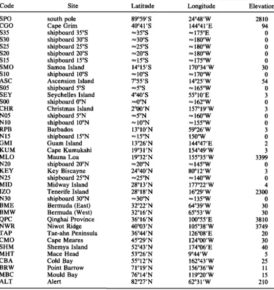
5054 CIAIS ET AL.' PARTITIONING OF OCEAN AND LAND UPTAKE OF CO: Table 1. Atmospheric CO2 Measurements at Network Land Sites

Code Site Latitude Longitude Elevation

SPO south pole 89o59 ' S 24ø48'W 2810 CGO Cape Grim 40ø41 'S 144ø41 'E 94 S35 shipboard 35øS •35øS • 175øE 0 S30 shipboard 30øS •30øS • 180øW 0 S25 shipboard 25øS •25øS • 180øW 0 S20 shipboard 20øS •20øS • 180øW 0 S15 shipboard 15øS • 15øS • 175øW 0 SMO Samoa Island 14ø15'S 170ø34'W 30 S 10 shipboard 10øS • 10øS • 170øW 0 ASC Ascension Island 7ø55'S 14ø25'W 54 S05 shipboard 5øS •5øS • 165øW 0 SEY Seychelles Island 4ø40'S 55ø10'E 3 S00 shipboard 0øN •0øN • 162øW 0 CHR Christmas Island 2ø00'N 157ø19'W 3 N05 shipboard 5øN •5øN • 160øW 0 N 10 shipboard 10øN • 10øN • 155øW 0 RPB Barbados 13ø10'N 59ø26'W 3 N 15 shipboard 15øN • 15øN 150øW 0 GMI Guam Island 13ø26'N 144ø47'E 2 KUM Cape Kumukahi 19ø31 'N 154ø49'W 3 MLO Mauna Loa 19ø32'N 155ø35'W 3399 N20 shipboard 20øN •20øN • 145øW 0 KEY Key Biscayne 24ø40'N 80ø12'W 3 N25 shipboard 25øN •25øN • 140øW 0 MID Midway Island 28ø13'N 177ø22'W 4 IZO Tenerife Island 28ø18'N 16ø29'W 2300 N30 shipboard 30øN •30øN • 135øW 0 BME Bermuda (East) 32ø22'N 64ø39'W 30 B MW Bermuda (West) 32 ø 16'N 65ø53 'W 30 QPC Qinghai Province 36ø16'N 100ø55'E 3810 NWR Niwot Ridge 40ø03'N 105ø38'W 3749 TAP Taeoahn Peninsula 36ø44'N 126ø08'E 20 CMO Cape Meares 45ø29'N 124ø00'W 30 SHM Shemya Island 52ø43'N 174ø06'E 40

MHT Mace Head 53ø26'N 9ø44'W 5

CBA Cold Bay 55ø12'N 162ø43'W 25

BRW Point Barrow 71ø19'N 156ø36'W 11

MBC Mould Bay 76ø14'N 119ø20'W 15

ALT Alert 82ø27'N 62ø3 I'W 210

separate

species

from total CO2 (12CO2

plus 13CO2).

The

accuracy of our calculations of the surface fluxes depends obviously on the quality of the transport model. The largest- scale aspects of the model transport have been validated

using

the tracers

85Kr and F-11. The vertical

mixing

in the

lowest two layers of the model may have been underesti- mated in the original version [Plumb and Mahlman, 1987]. In

this study

we have set 8 m 2 s -1 as the lowest

possible

value

for the vertical diffusivity in the lowest layer and likewise 6

m 2 s -1 as the lowest

value for the next vertical

layer (A.

also been made.

4. Description of the Isotopic Method

-1

The model outputs are the net surface fluxes, in GTC yr

(1 GTC - 1015

gC), of CO: and 13CO:

deduced

from the

S(x, t) and the flux of 13CO: as 13S(x, t). The inverse

calculation derives S(x, t) using only CO2 mixing ratio data,

whereas

13S(x, t) requires

both mixing

ratio and isotopic

data. The decomposition

of S and 13S into fossil fuel

emissions

(Sf and 13Sf),

net terrestrial

exchange

(St, and

13Sb)

, and

net ocean

exchange

(So and 13S

o) is expressed

by

section 4.3.

s = sa + so + So

13

S --. 13Sf

+ 13Sb

+ 13S

o

4.1. Fossil Fuels

Emissions

of fossil CO2 in the atmosphere

(Sf) are pre-

scribed in the model from monthly fuel consumption data of industrialized countries [Marland et al., 1985; Rotty, 1986;

Andres

et al., 1993].

The estimated

accuracy

of the Sf is

approximately 10%, which makes it the best known flux in the global carbon cycle. For 1990, 1991, and 1992 we used fossil emissions of 6.00, 6.07, and 6.10 GTC, respectively.

Emissions

of fossil

13CO2

(13Sf)

in the atmosphere

are

expressed as follows:

13Sf:

Rfmf

(3)

We prescribed

in the model the 13C/12C

ratio of fossil fuels

(Rf) according

to Andres

et al. [1993]. Each different

source

CIAIS ET AL.' PARTITIONING OF OCEAN AND LAND UPTAKE OF CO2 5055 -7.0 - -7.5 E

© -80

Point Borrow, Alaska

-7.0

E

8o

-8.5 -9.0

Mauna Loa, Hawaii

0 INSTAAR-NOAA/CMDL

• CSIRO-DAR

1990 1991 1992

Year

Figure 2. Comparison

of •13C measurements

on ai r samples

independently

collected

and analyzed

by

the Institute of Arctic and Alpine Research, University of Colorado (pluses) and CSIRO (diamonds). The curve is a fit to the data of the same type that we used in the deconvolution for every site.

of fossil CO2 is treated separately (oil, coal, natural gas,

flaring

and cement

production).

The •3C/12C

composition

of

oil, related to the region of production, ranges from -30%o to -26%o; flaring products average around -40%0. The

13C/12C

composition

of CO2 from the burning

of natural

gas

(-44%0) integrates both biogenic and thermogenic natural gas. Fossil CO2 released by cement factofids (0%o) and coal burning (-24.1%o) bears an isotopic signature largely inde-

pendent

of its geographical

origin.

The mean

value

of Rf in

the period 1990-1992 is -28.4%0 [Andres et al., 1993], significantly lighter than the commonly used value of -27.4%0 [Tans, 1981].

4.2. Terrestrial

13C

Exchange

Locally,

the net flux of 13C

between

the atmosphere

and

the terrestrial biosphere is the sum of two one-way fluxes, the photosynthetic uptake and the respiratory release. Plant

photosynthesis stores carbon from today's atmosphere, but

respiration releases carbon that has been locked up for some

period of time in plant tissues

and s0il organic

matter.

Because

the average

$13C of the atmosphere

has been

decreasing since the industrial revolution, "old" biospheric

carbon

that is respired

today is enriched

in 13C

compared

to

carbon that is incorporated into the biosphere today, de-

pending on its residence

time in the terrestrial biosphere.

Therefore even if the sum of biosphedc uptake and release of

CO2 is near zero, the sum of the 13C

fluxes

associated

with

photosynthesis and respiration is positive to the atmosphere.

We call this net isotopic enrichment of the atmosphere the "respiration isotopic disequilibrium." The CO2 respired by plants (from aboveground material and roots) bears the same

13C/12C

ratio as recent photosynthates,

so the fraction

of

COe that is cycled rapidly between atmosphere and plants

has no impact

on the annual

mean

atmospheric/513C.

"Old-

er" CO•, respired

by soil heterotrophic

processes,

is not in

isotopic

equilibrium

with the atmosphere.

This latter flux we

define as Sresp;

it is nearly equal to the uptake (Svh)

associated with net primary productivity (NPP), integrated

over a full year. The net exchange

of CO• and 13CO•

between the atmosphere and the terrestrial biosphere is given by

S b = --Sph q- Sresp

(4)

13S

b - - 13Sph

q- 13Sresp--

--OtphSphR

a q- OtbaSrespR

b (5)

where aph is the fractionation

associated

with plant photo-

synthesis (see section 4.2.3; the tissues of C3 plant are

depleted by about 17%o relative to the atmosphere and those

of C-4 plants by about 4%0); and aOa is the (negligible) fractionation associated with the respiration of CO2 by heterotrophic processes (a0a = 1).

4.2.1. Soil respiration disequilibrium. We rewrite (4) and (5) in order to make the isotopic disequilibrium of soil respiration appear explicitly, analogous to the air-sea ex-

5056 CIAIS ET AL.' PARTITIONING OF OCEAN AND LAND UPTAKE OF CO 2

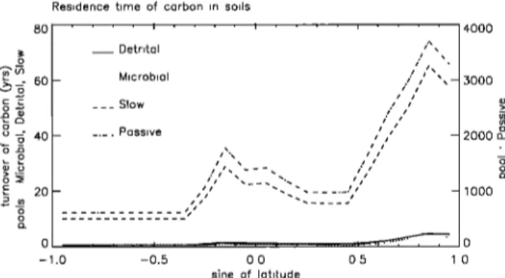
Residence time of carbon in soils 8O •,__- 60 -u_ •¾ 40 o o:• E .. 20- g o --.0 f T T __ Detrital

_

Microbial

2000

•--

Figure 3. Turnover of soil carbon as a function of latitude from global runs of the CENTURY soil model. Detrital and microbial soil carbon turns over in less than 10 years. Slow soil carbon turns over in about 100 years and passive soil carbon (right axis) in more than 1000 years.

as the 13C/12C

ratio of the atmosphere

that would be in

isotopic equilibrium with the biosphere [Enting et al., 1993, 1994; Tans et al., 1993].

R

abe

R

O

OZ ph

Replacing (4) and (6) into (5) we obtain

13S

b = OtphSbR

+ OtphSresp(R

b - Ra)

(7)

The heterotrophic respiration of CO2 by soils is then parti-

tioned into Npools,

pools of soil carbon

with different

turn-

over times (•i). Each pool accounts for a fraction (xi) of the total respiration flux:

Npools

Sresp--

Z iSresp

with

iSresp--

xiSresp (8)

i=1

Each pool of soil carbon retains an isotopic signature that

reflects

the isotopic composition

of atmospheric

CO2 when it

was originally photosynthesized. It is released to the atmo-

sphere

with a •3C/•2C

ratio iRb which

is the isotopic

ratio

of the atmosphere at the time of photosynthesis, multiplied

by

iRb = Ra(t - zi)

(9)

Replacing (8) and (9) into (7) we obtain

Npool

13Sb

= aphSbRa

+ aphSresp

E xi[Ra(t

- •'i) - Ra(t)]

i=1

= 13Sbe

q + 13Sbdis

(10)

Formally, (10) separates

the net flux of 13C between

the

atmosphere and the terrestrial biosphere into an "isoequi-

librium"

flux

(13Sbeq),

which

has

the same

isotopic

signature

as recent photosynthates and is proportional to the net flux

from the biosphere,

and an isodisequilibrium

flux (13Sbdis)

which differs from zero because the CO2 respired by soil bears an isotopic signature lagged by r i relative to recent photosynthates.

A further complication arises in forest ecosystems where

we also have to account for the residence time of carbon in

the aboveground biota prior to its delivery to the soil pool. We assume that metabolic material (leaves, stems) com- prises 70% of the litterfall, whereas structural material (fallen branches, logs) comprises 30% [O'Neill and De Angelis, 1981]. A turnover time of 50 years for forest structural carbon and 1 year for metabolic carbon yields an average turnover time of 16 years in the aboveground biota which adds to the turnover time in soils. Considering the

nonlinear

decrease

in atmospheric

8•3C since 1900 [Leuen-

berger et al., 1992; R. J. Francey, personal communication,

1994], this makes the 8•3C of litter in forests

0.12%o

higher

than today's atmosphere.

It is now well established that soil organic matter is comprised of fractions with multiple turnover times [Harri- son et al., 1993; Parton et al., 1987; $chimel, 1986]. The CENTURY ecosystem model [$chimel et al., 1994] uses four separate pools of carbon corresponding to detrital, microbial, slow, and passive carbon, respectively, in soils. Detrital and microbial pools consist of metabolic and struc- tural carbon compounds rapidly decomposed and recycled to the atmosphere in less than 10 years. The slow carbon pool consists of more resistant compounds, with a high lignin content, that turn over in 10 to 100 years2 The passive carbon pool turns over in more than 1000 years. $chimel et al. [1994] demonstrated that the turnover time of each pool is con- trolled by temperature and soil texture (Figure 3).

On the basis of the turnover time of carbon in soils and the

residence time of carbon in the aboveground biota, we

deduced

the 813C

of soil-respired

CO2 by using

the record

of

atmospheric

8•3C from measurements

over the last decades

[Keeling et al., 1989a] and by using ice-core data for earlier times [Leuenberger et al., 1992]. An additional complication

in determining

the exact 8•3C of litter arises

from the fact

that plants build their tissues during the growing season,

when 8•3C in the atmosphere

is generally highest. We

overcome this problem by replacing in equation (9) the latitudinal value of R a as deduced from the 1992 observa- tions, but weighted according to the seasonal flux of NPP [Fung et al., 1987]. Historical changes in the latitudinal

gradient

of 8•3C in the atmosphere

have been neglected.

Figure

4 shows

our estimate

of •13Cae

of CO 2 respired

by

each soil carbon pool, accounting for all the complications

outlined above.

Finally, we obtained the disequilibrium flux by using the

total heterotrophic

respiration

flux (Sresp)

from Fung et al.

[ 1987]

and the photosynthetic

fractionation

%,h as detailed

in

4.2.3. The soil respiration is distributed (fractions x i) among the different pools of soil carbon according to $chimel et al. [1994]. Table 2 below shows that the fractions xi do not exhibit large differences among the world biomes.

In summary, fast soil carbon (detrital and microbial pools) makes up about 80% of the heterotrophic soil respiration but

has a small isodisequilibrium

(less than +0.5%0). Slow soll

carbon makes up about 20% of the heterotrophic respiration

and can be up to + 1%o in disequilibrium. Passive soil carbon

bears the isotopic signature of preindustrial photosynthates (disequilibrium equal to + 1.5%o), but its contribution to the heterotrophic respiration is negligible. Generally, the dis- equilibrium of soil carbon increases with latitude in both hemispheres. In forest ecosystems the aging of structural plant tissues in the aboveground biota adds an additional disequilibrium to all pools of soil carbon of approximately

CIAIS ET AL.' PARTITIONING OF OCEAN AND LAND UPTAKE OF CO2 5057 Iso -6.0 T T T ' --6.0 - - --6.5 _ Detrital Microbial Slow -7 0 Passive _.. - -

Atmosphere

...

Figure 4. Disequilibrium of carbon respired by soils as a

function

of latitude

compared

to &]3C of the atmosphere

in

]992. The &]3C disequilibrium

of soil carbon is calculated

from the specific turnover time of carbon

aboveground

biota for forest

ecosystems.

•he &]•C of pho-

tosynthates is obtained by applying the discrimination by

plants to the &]•C of the atmosphere

duri• the •rowi•

S•ASOB. -7.0 -7.5 25 c• 15 O O ,_ ._ O_ E• '5• 10 5 -- ,0 Figure 5.

x

x

,,,/'"

i i

-0.5 0.0 0.5 .0 sine of Iotitude

Discrimination

against 13C by plant photosyn-

thesis (A) as a function of latitude. Values at high-latitude areas with no plants are extrapolated. The thick continuous line is the annual mean A inferred from global runs of the SiB model. In the two-dimensional inverse model, 12 different monthly maps of A are used; the thin line plots the average "growing season" A, mean from June to August. The dashed line is the annual mean A obtained independently by Lloyd and Farquhar [1994].

0.12%•.

Moreover,

as the 13C in plant tissues

reflects

the

atmospheric

513C

during

the growing

season,

a difference

of

about 0.2%• relative to the annual mean atmosphere has to be considered at high northern latitudes. The sensitivity of the model to the respiration isodisequilibrium is examined in

section 5.1.1.

4.2.2. Biospheric destruction disequilibrium. The de- struction of standing biomass in the tropics releases to the atmosphere carbon that has been stored in plant tissues for several years. Assuming that wood represents 60% of the aboveground biomass in tropical forests and that the average turnover time of carbon in the wood of tropical trees (rwt) is 50 years, we obtain a disequilibrium of approximately 0.7%• [after Leuenberger et al. 1992] for CO2 released by burning or deforestation in tropical forests. We assume that CO2 released by the frequent burning of tropical savannas is in isotopic equilibrium with the atmosphere. The biospheric destruction disequilibrium is expressed using (11).

13Sdes

dis

= aphSdes(Ra(t

-- rwt

) -- R.)

(11)

In (11) the flux of CO2 to the atmosphere due to biomass destruction in the tropics (S0e•) is taken from the global estimates of Houghton et al. [1987]. Note that we have not prescribed the gross biomass destruction in our deconvolu- tion; the net biomass destruction (forest burning minus regrowth) is a component of the total biospheric flux which is an output of the deconvolution. Provided that S&s does

not exceed 2-3 GTC (Sresp

is --30 GTC in the northern

hemisphere [Schlesinger, 1992]), the biospheric destruction disequilibrium in the tropics is about 10 times smaller that

Table 2. Distribution of Total Heterotrophic Respiration Among Different Pools of Soil Carbon (Fraction of Total

Flu x S r½sp)

Detrital Microbial Slow Passive Grasslands 0.50 0.30 0.20 <0.004 F ore st s 0.35 0.35 0.30 <0.004

the respiration disequilibrium at northern middle and high latitudes. Equation (11) should therefore be considered as a correction to the disequilibrium expressed by (10).

4.2.3. Discrimination

against

•3C by plant photosynthesis.

The assimilation of carbon by plants discriminates against

13C

because

of the enzymatic

preference

for •2C during

the

carboxylation

reaction

and because

13CO2

diffuses

more

slowly

than 12CO2

into the stomatal

cavity. The discrimina-

tion associated with the C-4 photosynthesis pathway is about 4%, relative to the atmosphere [Farquhar et al., 1989]. According to Farquhar et al. [1982, 1988] the discrimination (A) associated with photosynthesis by C-3 plants is described by

Ci

A = 4.4

+ (27.5

- 4.4)

Ca

(12)

where C, is the concentration of CO2 in the atmosphere, and Ci is the CO2 concentration in the stomatal cavity. The

photosynthetic

fractionation

factor (aph) is given by

O•ph-- 1

(13)

We derived monthly zonal averages of aph using the

values of C i calculated by the global biosphere model SiB [Sellers et al., 1986, 1988]. The SiB model is currently coupled with a general circulation model of the atmosphere and it fully accounts in a mechanistic manner for the interaction of plants with climate on a global scale, both for water and carbon [Sellers et al., 1992]. The value of C i is calculated from the carbon fluxes and stomatal opening at each time step of the model according to the algorithms developed by Collatz et al. [1991]. The SiB model has 11 different biomes, including three types of C-4 dominated biomes in the subtropics. We assigned to C-4 dominated biomes (mostly subtropical grasslands) an overall discrimi- nation of 15%, to account for patches of C-3 shrubs and trees. Figure 5 plots the annual mean zonally averaged discrimina- tion by plants as inferred from the SiB model. Larger discriminations, in the range 19-22%,, occur in temperate

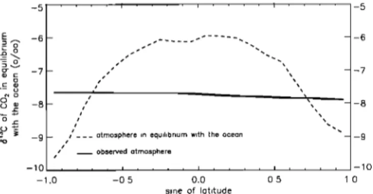
5058 CIAIS ET AL ß PARTITIONING OF OCEAN AND LAND UPTAKE OF CO2 -5 E --6 -- • ,-- -?• '- 0 o • -8- % -9 -10

atmosphere in equilibrium with the ocean

observed atmosphere I ... ... ß " ... x .0 -0.5 0.0 0.5 sine of latitude

-5 where Fao (Foa) is one-way flux of CO2 from (to) the

atmosphere;

Ro is •3C/•2C

ratio of ocean-dissolved

inor-

-6 ganic carbon

(DIC); a ao is atmosphere

• ocean fraction-

ation of •3CO2

(kinetic);

and aoa is ocean

• atmosphere

-7 fractionation

of •3CO2

(equilibrium

and kinetic).

Substitut-

ing (14) into (15) and defining

R•e tO be the •3C/•2C

isotope

-8 ratio of the atmosphere

in isotopic

equilibrium

with the

ocean,

-9

a oaRo

-10

R•e -

,

(16)

1.0 Ot ao

Figure 6. Ocean disequilibrium as a function of latitude.

Dashed

line is the $ •3C of the (hypothetical)

atmosphere

that

would be in isotopic equilibrium with the ocean. The con- tinuous line is the $•3C of the actual annual mean atmo-

sphere

in 1992

from the network

observations.

If the •i•3C

of

the atmosphere in equilibrium with the ocean lies above the

•i•3C of the actual atmosphere,

there is an outgassing

of

•3CO

2 from the ocean,

resulting

into a net isotopic

enrich-

regions of both hemispheres. Lower discriminations are

encountered in tropical regions corresponding to C-4 grass-

lands. The "growing season" discrimination (mean from June to August) is more relevant, because it corresponds to the period of assimilation of CO2 by plants. In temperate and boreal ecosystems where the assimilation is strongly sea- sonal, the growing season discrimination is on average lower than the annual mean by about 1%o (Figure 5).

Parallel to the SiB model, we have used another field of global isotope discrimination where Ci is derived in an empirical manner from a worldwide regression of physiolog- ical data [Farquhar et al., 1993; Lloyd and Farquhar, 1994]. The largest discrepancy between SiB and Lloyd and Farqu- har [1994] is found in regions where C-4 plants dominate (Figure 5). Especially at around 35øS, Lloyd and Farquhar [1994] find a zonally averaged discrimination of 10%o, whereas SiB predicts 18%o. In C-3 dominated biomes, the SiB discrimination is systematically larger than Lloyd and Farquhar [ 1994] (Figure 5), which may be due to the fact that the mesophyll resistance of plants is neglected in SiB (ap- proximating pCO2 in the chloroplast by pCO2 in the stoma- tal cavity). However, during the growing season, both esti- mates differ by 2-3%ø only. As an example, in temperate forests the discrimination estimated by Lloyd and Farquhar [1994] is 16-17%o and the value from SiB is 19-20%o. Both models predict a slight increase in the discrimination of C-3 plants when going from low to high latitudes, a pattern observed by K6rner et al. [1991] for plants growing at high altitude but not for lowland plants. The sensitivity of the inverse model to the discrimination by plants is examined in

section 5.1.2.

4.3. Ocean

•3C Exchange

In a manner similar to (4) and (5) for the biosphere we

express

the net CO2 and •3CO2

fluxes

between

atmosphere

and ocean using the notations of Tans et al. [1993].

S O = -Fao + Foa (14)

13S

o = --a aoFaoRa

-I--

a oaFoaRo

(15)

we obtain

13S

o = OtaoSoR

a + OtaoFoa(R•e-

Ra)= 13Soe

q + 13Sodis

(17)

Similar to (10) for the biosphere, (17) separates the air-sea

exchange

of •3C

into

an "equilibrium"

flux (•3So½

q) associ-

ated with a net transfer

of carbon and a flux (13Sodis)

associated

with

the isotopic

disequilibrium.

The flux 13Soe

q

bears practically the same isotopic signature as the atmo- sphere because the fractionation a ao associated with disso- lution of CO2 in the ocean is very small (2%ø). The flux

13Sodis

is proportional

to the disequilibrium

between

the

atmosphere and the ocean (R o _ R a ) Figure 6 plots R a ae ß

and the zonally averaged values of R o ae, as defined in (16), and shows that the ocean disequilibrium is approximately 2-3%ø. Physically, R•e differs from R a because the atmo-

sphere

mixes •3CO2

much

faster

than it can be transferred

from the ocean by air-sea exchange processes. The disequi-

librium

flux 13Sodis

is controlled

by the temperature

depen-

dence of the fractionation factor a oa and by the field of R o in

the ocean.

From Figure 6 it can be seen that 13Sodis

is

positive to the atmosphere (atmospheric enrichment) from the equator up to approximately 60 ø of latitude and negative beyond (atmosphere depletion).

To obtain the isotopic

disequilibrium

flux 13Sodis

, we

modeled the one-way flux of CO2 at the ocean surface (Foa) as the product of an air-sea gas transfer coefficient (which depends on seasonally varying wind speeds [Tans et al., 1990]), and global measurements of ApCO2 from Takahashi et al. [1986]. The total one-way flux F oa obtained in this

manner

is equal

to 85 GTC yr -1 . We used

the parameteriza-

tion of Otoa derived by Tans et al. [1993] from separate

laboratory

determinations

of the •3C fractionation

among

HCO•-, CO32-,

and atmospheric

CO2, respectively

[Lesniak

E oa = k 0 + k•(T + k2)T

2

-10.66; k• = +0.1196; and k 2 = -3.095 x 10 -4.

We estimated the zonally averaged distribution of R o in the world ocean from measurements on ship cruises com- piled by Tans et al. [1993]. The data are from Geochemical Ocean Sections Study [1987], Kroopnick [1980, 1985], and Quay et al. [1992]. Considering the progressive invasion of the ocean by isotopically depleted CO2 [Quay et al., 1992],

CIAIS ET AL.' PARTITIONING OF OCEAN AND LAND UPTAKE OF CO2 5059

one must be careful in merging R o measurements of water

samples collected in different years. We inferred the distri- bution of R o for the period 1990-1992 from the distribution

in 1980 adjusted

by a decreasing

trend of -0.01%o yr -i.

Another complication concerns the seasonal variations in R o

controlled by marine biological activity, the rate of upwelling

of nutrient-rich,

13C depleted

deep waters, and to a lesser

extent by air-sea exchange (a very slow process). We derived a rough order of magnitude value of the summer

enrichment

in 13C of surface

waters

due to phytoplankton

productivity alone as follows' Removing from 55% of the

world surface

waters

(1000

GTC with an average

winter •i

of + 1.5%o) a fraction 75% of the global new production (15

GTC with an average

•il3C of -20%o) [Berger

et al., 1989;

Tans et al., 1993], we obtain a summer R o value of about 2%o, thus enriched by 0.5%o compared to the winter. How- ever, in this study we assumed that the slow kinetics of the

air-sea

exchange

of 13CO2

prevents

such

a seasonal

signal

in

R o from entering the atmosphere. The disequilibrium flux was therefore prescribed by using the annual mean values of R o. The sensitivity of the inverse model to the ocean isotopic disequilibrium is discussed in section 5.1.2.

4.3. Partitioning CO2 Between Ocean and Land Ecosystems

To infer the partitioning of CO2 between ocean and land, we want to calculate the fluxes So and So in the set of

equations

(1) and

(2). Replacing

13Sf

using

(3), and 13S

0 and

13S

o with (10) and (17), in the set of equations

(1) and (2)

yields a simple linear system (20) for So and S 0, which we

can solve for each latitude and time.

aaoRa aphRa/t

[Sbj

s

- sf

)

= 13 (20)

13S- SfRf- 13Sbdis-

13Sdefdis-

Sodis

The solutions are

S b =

OtaogaS

q-

(gf- Otaoga)S

f- 13S

q- 138bdis

q- 13Sodis

q- 138defdis

(aao -- aph)Ra

(21) So ---

aphRaS

+ (gf- aphga)S

f-- 138

+ 138bdis

+ 13Sodis

+ 138defdis

(a ao -- aeh)Ra

(22) Note that So and So are functions of the surface fluxes (S and

13S)

derived

from the inverse

atmospheric

transport

model

and depend only on a limited set of parameters: the fraction-

ation factors

aph and aao and the isotopic

disequilibria

S odis,

Sbdis , and Sdefdis. The sensitivity of the model to the

discrimination by plants and to the disequilibria is examined in the next section. We did not investigate in detail the sensitivity to the fossil fuel terms, which are supposed to be accurate to 10%. Our approach requires no "missing sink" to balance the global carbon budget as it inverts the obser- vations directly. The sum of S O and So always equals the

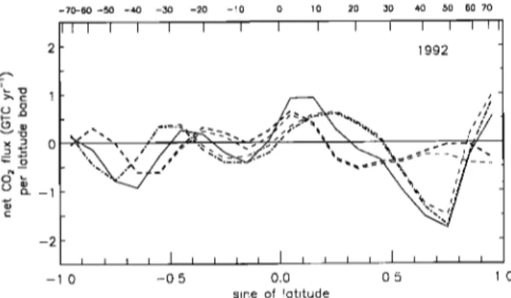
• 0 -2 Stondord Run -70-60-50 -40 -30 -20 -10 0 10 20 30 40 50 60 70 1992 .0 -0.5 0.0 0.5 1.0 sine of Iotitude

Figure 7. Latitudinal ocean/land partitioning of the sources and sinks of CO2 versus latitude in the standard run

of the deconvolution.

Units are GTC yr -1 per latitude

band

of the model (20 bands total). The continuous line is the net flux of CO2 after removal of fossil fuels. The dashed line is the net flux of CO2 exchanged with the oceans. The dashed- dotted line is the net flux exchanged with land ecosystems. The sum of ocean and land fluxes equals the total net flux of CO 2 ß

total net flux S, which is inferred from the inversion of the

CO2 mixing

ratio data alone. If, for example,

the •il3C data

"force" the model to overestimate the flux into the ocean at

a given latitude, it will be at the expense of the flux into the terrestrial biosphere.

5. Results and Sensitivity Study

In the standard run of the model, all sites available are used to constrain the inversion, all disequilibria are pre-

scribed

as detailed

above, and the discrimination

of 13C by

plants is from the SiB model. The model is initialized in a

5-year

run using

813C

data measured

by CSIRO since

1985

at

SPO, CGO, MLO, and BRW [Francey et al., 1990] and the corresponding CO2 data at these sites from NOAA/CMDL [Conway et al., 1994]. Figure 7 plots the annual mean latitudinal pattern of the CO2 sources and sinks. Units for

net fluxes

in Figure 7 are GTC yr --1 per latitude

band of the

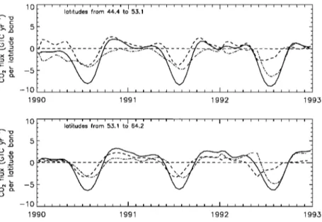
model. Figure 8 plots the seasonality in the tropics. Figure 9 plots the seasonality in the northern hemisphere and Figure 10 for the Arctic. We first examine the sensitivity of the

model in section 5.1 in order to estimate errors associated

with the ocean/land partitioning. We then discuss the latitu~ dinal patterns in section 6.1, the seasonality in section 6.2, and the global patterns in section 6.3.

5.1. Sensitivity Study

5.1.1. Sensitivity to the biospheric disequilibria. We compared the standard run with a run in which the bio- spheric disequilibrium is set to zero (experiment 1). Figure 11 plots the latitudinal pattern of the CO2 sources and sinks in this experiment. Experiment 1 underscores the impor- tance of the biospheric disequilibrium in forest ecosystems. Compared to the run with no disequilibrium, the standard run has a smaller terrestrial uptake in the northern hemi- sphere as well as in the southern tropics. In the northern hemisphere this is because both the turnover of soil carbon is long (Figure 3) and the release of CO2 from the soils is important during the summer [Fung et al., 1987]. On land