Working long hours: less productive but less costly? Firm-level evidence from Belgium

RESEARCH OUTPUTS / RÉSULTATS DE RECHERCHE

Author(s) - Auteur(s) :

Publication date - Date de publication :

Permanent link - Permalien :

Rights / License - Licence de droit d’auteur :

Bibliothèque Universitaire Moretus Plantin

Institutional Repository - Research Portal

Dépôt Institutionnel - Portail de la Recherche

researchportal.unamur.be

Working long hours: less productive but less costly? Firm-level evidence from Belgium

Delmez, Françoise; Vandenberghe, Vincent

Publication date:

2017

Document Version

Publisher's PDF, also known as Version of record

Link to publication

Citation for pulished version (HARVARD):

Delmez, F & Vandenberghe, V 2017 'Working long hours: less productive but less costly? Firm-level evidence from Belgium' IRES Discussion Papers, no. 2017-22. <https://sites.uclouvain.be/econ/DP/IRES/2017022.pdf>

General rights

Copyright and moral rights for the publications made accessible in the public portal are retained by the authors and/or other copyright owners and it is a condition of accessing publications that users recognise and abide by the legal requirements associated with these rights. • Users may download and print one copy of any publication from the public portal for the purpose of private study or research. • You may not further distribute the material or use it for any profit-making activity or commercial gain

• You may freely distribute the URL identifying the publication in the public portal ? Take down policy

If you believe that this document breaches copyright please contact us providing details, and we will remove access to the work immediately and investigate your claim.

Working long hours: less productive

but less costly?

Firm-level evidence from Belgium

F. Delmez and V. Vandenberghe

Discussion Paper 2017-22

Working long hours: less productive but less costly?

F. Delmez* _{& V. Vandenberghe}£

Abstract

From the point of view of a profit-maximizing firm, the optimal number of working hours depends not only on the marginal productivity of hours but also on the marginal labour cost. This paper develops and assesses empirically a simple model of firms' decision making where productivity varies with hours and where the firm faces labour costs per worker that are invariant to the number of hours worked: i.e. quasi-fixed labour costs. Using Belgian firm-level data on production, labour costs, workers and hours, and focusing of the estimation of workers/hours elasticities of isoquant and isocost, we find evidence of the declining productivity of hours, but also of quasi-fixed labour costs in the range of 20% of total labour costs. We also show that industries with larger estimated quasi-fixed labour costs display higher annual working hours and make less use of part-time contracts. The tentative conclusion is that firms facing large quasi-fixed labour costs are enticed to raise working hours (or oppose their reduction), even if this results in lower labour productivity.

Keywords: men vs hours, working hours, imperfect substitutability, labour costs

JEL Codes: J22, J23, C13

* Economics Department, University of Namur, Rue de Bruxelles 61, B-5000 Namur Belgium. email:

francoise.delmez@unamur.be.

£ Economics Department, IRES, Economics School of Louvain (ESL), Université catholique de Louvain

(UCL), 3 place Montesquieu, B-1348 Belgium. email : vincent.vandenberghe@uclouvain.be.

Both authors thank Marion Collewet for her many useful and encouraging comments on previous versions of this paper. F. Delmez gratefully acknowledge funding from the Belgian Fund for Scientific Research (FNRS).

2 A renewed interest in reducing working hours has recently been observed in many countries. In the wake of the 2008 crisis, it has been proposed to combat surging unemployment. It is also seen as a desirable corollary to longer careers (i.e. part-time/gradual retirement schemes) that governments promote in response to population ageing. The canonical model of labour supply states that a worker can flexibly choose his/her own work hours to maximize his or her utility at any given wage.1 _{However, findings from several studies, reviewed by Kuroda &Yamamoto}

(2013), suggest that workers cannot choose work hours freely, or that a change of hours is conditional on a job change.2 In this context, and following Pencavel’s call (Pencavel, 2016) for more research on the demand of labour3_{, this paper focusses on the preferences of firms}

regarding the working hours of their employees.

In fact, once that intensive dimension of labour is introduced, firms must make a non-trivial decision on the number of workers hired as well as on the hours that are asked from them. A profit-maximizing firm will decide on the number of workers to hire and on working hours by comparing the productivity and cost of both workers and hours. Labour productivity, whether at the intensive or at the extensive margin, has already attracted a lot of interest in the past. A first, rather old, stream or the economic literature develops the idea that longer hours lead to counterproductive hardship. John Hicks (1932) stated that “probably it has never entered the heads of most employers…that hours could be shortened, and output maintained.” A milder version of his story is that, as workers slave away for longer and longer, they lose energy, which makes them relatively less productive: in other words, the last hours of work still raise total output but at a declining rate. In contrast, Feldstein (1965) insists on the importance of "slack" hours. He argues that many hours amount to setting-up time, refreshment breaks, time around lunch… and deliver no output. These paid-but-non-productive hours do not rise proportionately with the number of hours officially worked. An increase in the length of the official working day or week could therefore entail a more than proportionate increase in the number of effective hours of works. Our empirical work follows the conclusions by Leslie & Wise (1980), or more recently by Pencavel (2015) or Collewet & Sauermann (2017) that give credit to the hardship story, but it in its mild form: average productivity of hours is decreasing in the number of hours, due to the decreasing marginal productivity. This result is however only valid at the observed number of hours worked and does not contradict the presence of slack hours for lower number of hours worked.

So, could it be that employers have it all wrong when they oppose reducing working hours even though it could boost productivity? Not necessarily if, as proposed by Oi (1962), Donaldson & Eaton (1984), Dixon & Freebairn (2009) or Kuroda &Yamamoto (2013), the existence of quasi-fixed labour costs is considered. The main contribution of this work is to shed light on the role of quasi-fixed labour costs in understanding firms' demand for hours.

The notion deserves some clarification. Fixed costs of production already benefited from attentive scrutiny in the economic literature. They are usually understood as any financial cost

1 Workers' preferences regarding hours have largely been studied in previous work (see for example Barzel 1973, Freeman & Gottshalk 1998 and more recent work by Rogerson, Keane & Wallenius (2009, 2011, 2012) 2 For example, in his survey on labor supply, Heckman (1993) concludes that most of the variability in labor supply can be explained by extensive margins (i.e., worker flows into and out of the labor market), whereas intensive margins (i.e., changes in hours worked) are extremely small. Using job-mover data, Altonji & Paxson (1986, 1988, 1992) or Senesky (2004) suggest that choices of wages and hours are available only as a ‘‘package’’; therefore, a worker is not able to change work hours flexibly unless he or she changes jobs. 3 The relative importance of the demand for labour has also been highlighted by Bryan (2007) and Stier &

3 – most often corresponding the cost of capital – not dependent on the level of goods or services produced. Less often explored, quasi-fixed labour costs are the focus of this paper and arise from the explicit modelling of both the intensive and the extensive margin of employment. Here, following Hamermesh’s (1993) typology, quasi-fixed labour costs (F) reflect the propensity of a worker's compensation to be not strictly indexed on the hours of work delivered (H) [but rather on the number of workers N]. That comprises the lump-sum part of pay, non-proportional taxes or social security contributions, fixed insurance premia, indivisible perks like company car, but also recruitment/training or redundancy/firing costs…

Hamermesh distinguished two types of quasi-fixed labour costs. First, the “recurring fixed costs” (R). These are the costs associated with nonwage remuneration and fringe benefits: the health insurance, leasing car, paid sickness leave (as well as any other type of leave where the worker remains paid while not delivering any hour). Second "one-time fixed cost" (T). In Hamermesh's typology these are costs that are paid only once per worker. They typically consist of the cost of (externally or internally provided) training, the cost of operating an HR department, and dismissal costs. At the level of a firm, the one-time fixed costs will enter F pro rata the likelihood q of turnover F=R+qT. By contrast, variable labour costs are those that vary with the number of hours; and will typically correspond to the product of hours by an hourly wage rate (w(H)H). The total labour cost of a typical firm thus writes C(N,H)= N[w(H)H + F]. In the presence of significant labour fixed costs (F), raising the number of hours per worker will decrease the average cost and raise profitability ceteris paribus.

Evidence gathered in this paper, using firm-level data covering the wholeBelgian private for-profit economy, suggests both a declining productivity of hours, and a declining average cost per additional hour worked. Using annual firm-level data over a 9-year period (2007-2015), we show that in the Belgian private economy firms operate around a level of hours per year that is synonymous of decreasing average productivity: thus, shorter hours could have a positive effect labour productivity (value-added per hour). But analysing the relationship between total labour cost and hours, we also find strong evidence of substantial quasi-fixed labour costs (around 20-23% of total labour costs) suggesting that maximizing firms have an incentive to push hours beyond the point where labour productivity is maximal. To our knowledge, this paper is the first to examine empirically both the question the productivity of hours and that of their role in coping with quasi-fixed labour costs. It is also the first to estimate econometrically (instead of just reporting what accounting data reveal) the share of quasi-fixed costs.

One of the tentative conclusions of the paper it that, akin so many other aspects of economic life, the decision of firms on working hours amounts to a trade-off: reducing working hours might improve labour productivity, but it could also raise average labour cost per hour. A better understanding of firms' or industries' incentives to reduce or raise working hours should help policy making. For example, to promote part-time employment for the older workers, policy makers should prioritize industries with low quasi-fixed labour costs or foster tax and compensation policies that ensure that employer costs are as proportional as possible to hours of work.

The rest of the paper is organized as follows. Section 1 exposes a model of the profit-maximising firm that has all power to decide on the number of workers, but also on the number of hours each worker must work. The model highlights the likely determinants of the demand for workers and working hours, the role of the productivity of hours and that of quasi-fixed labour costs. It also suggests a way to identify econometrically the share of fixed labour costs as the workers/hours elasticity along the isocost. Section 2 describes the panel of firm-level data

4 that is used. Section 3 exposes our econometric analysis and results. We first present baseline estimates of the productivity of working hours and of the share of quasi-fixed labour costs in total labour costs. Second, we introduce an industry-by-industry analysis that shows that industries with larger quasi-fixed labour costs tend to have higher average working hours higher and make less use of part-time work. Section 4 exposes a certain number of robustness checks. Section 5 exposes the economic and institutional mechanisms that in the Belgian context generate quasi-fixed labour costs. Section 6 concludes.

1. Working hours as a firm-level decision

Consider a technology where effective labour consists of hours (H) and worker (N), where hours of presence (H) do not equal effective hours of labour g(H). The production function is as follows:

𝑄𝑄(𝐾𝐾, 𝐿𝐿) = 𝑓𝑓(𝐾𝐾, 𝐿𝐿) [1.]

𝐿𝐿 = 𝑁𝑁𝑁𝑁(𝐻𝐻), 𝑁𝑁′(𝐻𝐻) > 0 [2.]

Assuming that g(H)=H for every possible value of H is probably unrealistic. Doubling hours per worker will not double the amount of effective hours/labour. As soon as one lifts the assumption of identity, the labour demand can no longer be simply considered as employers just choosing an optimal number of worker-hours (i.e. the product N.H equal to L) (Hamermesh (1993)) – with the level of H being essentially a matter of workers' preferences in terms of revenue versus leisure. In this model we make the opposite assumption that employers are free to choose the number of hours worked per worker as well as the number of workers. It is worth noting that the specific form for L(N,H) will lead to the absence of scale effect on H*: hours worked per worker are independent of the size of the firm (measured by N).

Following Cahuc et al. (2014), we assume firms face the following sequence of choices: first, firm choose between hours and workers by minimizing their labour cost, second they choose between labour (optimally composed of hours and workers) and capital. This sequential choice hypothesis implies that hours versus workers decisions are invariant to firm size and therefore separable from capital4. The employers' problem can then be viewed as one of minimizing total labour cost C(N,H) subject to the technological constraint Y≤ f(K, Ng(H)). The optimum (H*,N*) is described by a series of FOC that lead after some manipulations to equating the ratio of marginal productivities to the ratio of marginal labour costs:

𝐿𝐿𝐻𝐻

𝐿𝐿𝑁𝑁

=

𝐶𝐶𝐻𝐻

𝐶𝐶𝑁𝑁 [3.]

or equivalently using [2] and assuming that the true generating process for labour cost is:

𝐶𝐶(𝑁𝑁, 𝐻𝐻) = 𝐹𝐹𝐹𝐹 + 𝑁𝑁[𝑤𝑤(𝐻𝐻)𝐻𝐻 + 𝐹𝐹] [4.]

4 The sequence of choice has been documented before and it seems realistic to think that capital/labour ratio decisions are subject to a different timing than hours/workers decisions. Would this assumption be lifted, the final signs of derivatives would be indeterminate and depend on capital, workers and hours complementarity (Hart, 1984).

5 where

w(H) is the hourly wage (“variable labour costs”) and rises with H (w'>0) to reflect, among other, the legal obligation to pay more for extra hours. Modelling the overtime premium as a continuous increasing hourly wage function allows to compute elasticities that we will be able to estimate in the dataset. The alternative modelling option is to have an overtime premium paid per hour above a legal threshold, however our data would not allow us to estimate the increase in remuneration at the threshold5_.

F are labour quasi-fixed costs (i.e. costs that are invariant to the number of hours per worker, but vary with the number of workers). A version of the model explicitly modelling quasi-fixed costs as non-proportional to hours worked instead of perfectly fixed is presented in Appendix A. The key predictions of the model remain unchanged. FF are firm-level fixed costs (i.e. costs that are invariant to the number of workers (human resources personnel, administrative procedures vis-à-vis insurers, public authorities…)). we get 𝐿𝐿𝐻𝐻 𝐿𝐿𝑁𝑁

=

=

=

One can also restate the equilibrium using the implicit function theorem6, where the ratio of marginal productivities 𝐿𝐿_𝐻𝐻⁄ is equal to the slope of the isoquant: 𝐿𝐿_𝑁𝑁

−

𝐿𝐿𝑁𝑁

=

𝑑𝑑𝑁𝑁

𝑑𝑑𝐻𝐻│𝑑𝑑𝐿𝐿=0 [6.]

And multiplying by 𝐻𝐻 𝑁𝑁⁄ leads to the elasticity along the isoquant σ(H, N):

−

=

Similarly, the ratio of hours and men marginal labour cost 𝐶𝐶_𝐻𝐻⁄ can be related to the elasticity 𝐶𝐶_𝑁𝑁 of substitution along the isocost 𝛾𝛾(𝐻𝐻, 𝑁𝑁):

−

=

Thus, as alternative to [3], the optimum N*, H*can be described as the equality of the slopes of the isoquant/isocost in the (N, H) space; or the equality of the elasticities of hours per worker along both the isoquant and isocost (Dixon et al., 2005):

𝜎𝜎(𝐻𝐻, 𝑁𝑁) = 𝛾𝛾(𝐻𝐻, 𝑁𝑁) [9.]

5 In fact, modelling labour cost as wH + p(H-H0)+ F will lead to the right-hand side of equation to 5 to simply

be the ratio of variable over total cost per hour worked for all H>H0. 6 _{dL=0= LH dH+ LNdN}

6 or equivalently, given [2] and [4]:

𝜎𝜎(𝐻𝐻, 𝑁𝑁) = 𝑁𝑁_𝑁𝑁′((𝐻𝐻𝐻𝐻)) 𝐻𝐻

=

the elasticity of hourly wage to working hours;

𝑟𝑟𝐹𝐹 ≡ _{𝑤𝑤(𝐻𝐻)𝐻𝐻}𝐹𝐹 the ratio of fixed to variable worker-level labour costs.

Note incidentally that if 𝜀𝜀 = 0 (i.e. hourly wages are not affected by H), then, assuming [4], (1 − 𝛾𝛾(𝐻𝐻, 𝑁𝑁)) boils down to [1 − (1 (1 + 𝐹𝐹 𝑤𝑤(𝐻𝐻)𝐻𝐻⁄ ⁄ ))] or equivalently [𝐹𝐹 (𝐹𝐹 + 𝑤𝑤(𝐻𝐻)𝐻𝐻⁄ )]. Hence, the more 𝛾𝛾(𝐻𝐻, 𝑁𝑁) is inferior to 1, the higher the share of fixed costs in total labour costs. In what follows, [1 − 𝛾𝛾(𝐻𝐻, 𝑁𝑁)] will interpreted as a (lower-bound) estimate of the share of quasi-fixed labour costs in total labour costs.

Equation [10] means that H* is such that the ratio of its marginal to average productivity [𝑁𝑁′_{(𝐻𝐻) 𝑁𝑁(𝐻𝐻) 𝐻𝐻⁄ ⁄ ] equals [1 + 𝜀𝜀(𝐻𝐻) 1 + 𝑟𝑟𝐹𝐹⁄ ]. The higher fixed costs relative to the sensitivity} of wage rate to hours, the more likely 𝛾𝛾(𝐻𝐻, 𝑁𝑁) will be inferior to 1 (in absolute value). Simultaneously, if that is the case employers will push for longer hours; certainly, beyond the point where marginal productivity starts declining (presumably due to hardship, lassitude…), and beyond the point where average productivity of hours reaches its maximum (Figure 2)7_.

Said differently, the only reason for firms to push working hours to the point where average productivity is declining, is that they must recuperate fixed costs.

This finally leads to positing that the (conditional) labour demand for working hours looks like:

𝐻𝐻∗ _{≡ 𝑚𝑚 �𝑄𝑄⏞}+_{, 𝜎𝜎⏞}−_{� = 𝑛𝑛 �𝑄𝑄⏞}+_{, 𝛾𝛾⏞}−_{� = 𝑛𝑛(𝑄𝑄⏞}+_{, 𝐹𝐹⏞}+_{, 𝜀𝜀⏞}−_{) [11.]}

7 Mathematically, the sign of the slope (or derivative) of the average productivity is determined by the difference between the average productivity and the marginal productivity. It the latter is smaller than the former (i.e. if

σ(H)<1) we necessarily have a negative slope for the average productivity, meaning that we are beyond its

7 Figure 2 – Optimal hours, ratio of marginal to average productivity of hours and quasi-fixed labour costs (F1>F0)

2. Data

The data we use in this paper essentially come from Bel-First (Tables 1, 2, 3 and 4, Figures 1a and 1b),8 that all for-profit firms located in Belgium must feed to comply with the legal prescriptions on income declaration. It consists in a large unbalanced panel of 115,337 firm-year observations corresponding to the situation of 14,544 firms with at least 20 employees, from all industries forming the for-profit Belgian private economy9_{, in the period 2007–}

201510. Our dataset comprises a large variety of firms. First along the firm size dimension, we include all data for firms from 20 workers (FTE) to very large firms (above 1,000 workers), corresponding to well-known international companies11. These firms are largely documented in terms of industry (NACE12 _{or NAICS}13_{), size (number of workers), capital used (total}

equity), total labour cost (more on this below) and productivity (value added).

Descriptive statistics on this large sample are reported in Tables 1 to 4. One of the originalities of this paper is to consider both the productivity and the labour cost of hours and workers. Table

8 http://www.bvdinfo.com/Products/Company-Information/National/Bel-First.aspx

9 We remove the primary sector (agriculture and mining) as well as the public/non-profit industry (NACE 1-digit codes "A","B","O","P","T","U").

10 The analysis has also been performed on 2005-2014 data without any impact on the conclusions.

11 Such as Volvo, Arcelor, Audi, GSK, Electrabel, Colruyt, Delhaize, Carrefour, AIB-Vinçotte and 10 large interim firms (Randstad, Adecco, Start People, T-Groep, Tempo Team, Daoust, Manpower, …).

12 European industrial activity classification (Nomenclature scientifique des Activité économiques dans la Communauté Européenne)

13 North American Industry Classification System (NAICS)

H H g’(H) marginal productivity g(H)/H average productivity H H σ= g’(H)/(g(H)/H) H*F0 1 𝛾𝛾 =(1+ε(H))/(1+rF0) 𝜸𝜸 =(1+ε(H))/(1+rF1) H*F1 Productivity in value σ and 𝜸𝜸 in value

8 2 contains descriptive statistics on productivity (Q/N where Q is value-added) and average labour costs (C/N). The latter is logically inferior to productivity.

In this paper, labour costs are measured as a firm-level aggregate independently from production. They include the value of all wage and nonwage compensations paid to or on behalf of the total labour force (both full- and part-time plus interim/temporary workers) on an annual basis. Labour costs comprise: annual gross wage (including end-of-the year bonuses, paid holiday/sickness/maternity leave), employees' social contributions (representing 13.07% of gross wage), employers' contributions to social security (38% of the gross wage), employers' contributions to extra-legal insurances and pensions, stocks and other (taxable) perks like "meal vouchers", company car, mobile phone… Most of the costs of externally provided training are included in the firms' total labour cost used here14.

And so are Belgium's notoriously high severance payments including the special regimes applicable to older workers15 16.

All in all, the firm-level aggregate that we use is thus likely to capture most of the "recurrent" and "one-time" quasi-fixed costs mentioned in the introduction. Still there is a need of an in-depth analysis of which of these items can be considered as genuinely "fixed" (see Section 5 for this). An exception are recruitment/search costs and those of internally provided training are unlikely to be included as they are not ascribed to workers and appear in the books as intermediates. Internal training costs, as well as those of HR departments involved in search and recruitment are unlikely to appear in our data a fixed labour costs. This is because they essentially take the form of wages paid to specialised workers (who also deliver a certain number of hours); just like any other employee of the firms. In our data, there is no way to isolate their labour cost.

Of crucial importance in this paper is the distinction between the number of workers (N) and the number of hours (H) (Table 2 right-hand columns, Table 3). The former is simply the headcount, or more precisely the average over the year of the headcount at the end of each month. The latter corresponds to the number of worked and paid hours over the year17. It does not consider unpaid overtime, holidays, sick leaves, short-term absences, and hours lost due to strikes or for any other reasons.

The average hours worked varies strongly in our sample; even within full-time workers (Figure 1a,b). The standard deviation of hours worked (overall or for full-time workers only) within firm is only slightly smaller than between firms (Table 4). Generally, we observe non-negligible variation of both hours and workers within firm, over time representing more than

14 Account 648 "Other Personnel Expenses";

15 By contrast, the cost of workers in a pre-retirement scheme are not counted anymore when fully retired. If partially retired (“aménagement de fin de carrière”), they count as part-time workers; and the worker replacing them for the other part-time is counted.

16 Unemployment with complement paid by the former employer ("complément d’entreprise"); account 624 Retirement and survival pensions.

17 Unlike hours found in the social security database, Belfirst data on hours do no suffer from the "assimilation" bias: i.e. hours that are assimilated to worked hours in the definition of social (e.g. pension) rights. The only serious issue with Bel-first is thus the underestimation of worked hours due to unpaid overtime (something this seems to be common among white collar workers).

9 30% of total variation18. This observation of large within-firm variations is important to allow form meaningful firm-level fixed effects regressions in the subsequent econometric analysis. In the extension of the main econometric analysis (Section 4) we also use individual-level international data from PIAAC19.

Table 1: Bel-first. Number of firms

Year Number of firms 2007 11,944 2008 12,213 2009 12,369 2010 12,698 2011 12,949 2012 13,272 2013 13,365 2014 13,370 2015 13,157 Nobs 115,337 Total #firms 14,544 Source: Bel-First (2016)

Table 2: Descriptive statistics, main variables

Year Avg Value added per empl. Q/N [EUR] Avg Labour cost per empl. C/N [EUR] Avg Capital per empl. [EUR]

Hours and workers (mean) Hours per empl. [annual] H Workers full time N ft Workers part time N pt Workers interim/temp N int 2007 77,133.03 43,237.04 325,163.3 1,472.4 80.38 24.78 14.57 2008 78,996.69 44,680.06 413,030.7 1,472.4 80.77 24.83 12.98 2009 73,856.15 45,153.60 426,619.2 1,428.4 76.80 24.97 11.51 2010 76,494.41 45,898.61 322,024.1 1,433.2 74.66 25.57 12.59 2011 79,430.76 47,709.65 610,067.9 1,437.2 76.33 27.14 12.28 2012 76,136.48 49,003.94 639,064.7 1,427.9 75.78 28.02 12.57 2013 76,403.06 49,705.03 485,220.0 1,422.4 75.44 29.02 12.81 2014 77,347.08 50,599.59 462,562.8 1,427.7 90.82 36.38 12.37 2015 79,568.47 50,779.37 329,668.3 1,430.1 75.33 37.95 13.67 All years 77,269.98 47,517.51 447,715.7 1,438.5 78.49 28.87 12.81 N obs 115,337 Source: Bel-first (2016)

18 Even after removing outliers: i.e. firms declaring hours per worker to be, on average over all workers, below 100 or above 3000 annual hours, mostly due to encoding errors.

10 Table 3: Descriptive statistics, Workers and hours: details (percentiles).

Moment Number of workers. (N) Av. hours [full-time w.] (H ft) Av. hours [part-time w.] (H pt) Av. hours [interim w.] (H int) Share of full-time w.$ Share of part-time w. $ Share of interim w. $ p25 27.00 1,464.92 857.25 1,634.33 0.68 0.06 0.00 p50 40.00 1,581.86 1,044.60 1,883.59 0.83 0.12 0.00 p75 74.00 1,666.90 1,201.75 2,004.15 0.92 0.27 0.03 p99 1,169.00 2,438.83 1,859.00 2,742.00 1.00 0.97 0.33 Mean 112.06 1,563.63 1,022.38 1,791.26 0.75 0.22 0.03 Nobs 115,337

Source: Bel-first (2016), $ in total number of workers

Figure 1a- Annual average working hours per worker. Distribution across firms. Belgium private economy 2007-2015.

11 Figure 1b- Annual average working hours per worker [full-time workers only]. Distribution across firms. Belgium private economy 2007-2015

Source: Bel-first (2016)

Table 4 – Importance of within [over time] vs between [across] firm variation of employment and hours Number of workers (N) Working hours (H) Working hours FT (HFT)

Std_error (between) [a] 454.15 281.62 207.00

Std_error (within) [b] 686.73 185.31 188.67

Within share of total var. [b]2_/([a]2_+[b]2₎

0.696 0.302 0.454

Source: Bel-first

3. Econometric analysis of firm-level data

In this section, using firm-level panel data, we estimate both production and labour cost functions20 _{with the aim of assessing the productivity of working hours and the (relative)}

importance of quasi-fixed labour costs. We do so using firm level data and, in a robustness analysis, using individual-level international data. The latter can only be used to detect the presence of quasi-fixed labour costs (see Section 4.1) by exploiting the cross-individual variation of the number of hours. The advantage of firm-level data is that workers and hours can be analysed simultaneously. And as the data consist of panels, they can be used to control for firm-level unobserved heterogeneity as well as for the risk of simultaneity bias (both being

20 Not to be confounded with a the traditional [production] cost function i.e. a function of input prices and output quantity.

12 synonymous to endogeneity). What is more, the dataset is sufficiently large to allow for: i) the identification of cross-industry differences (in terms of 𝜎𝜎(𝐻𝐻, 𝑁𝑁), 𝛾𝛾(𝐻𝐻, 𝑁𝑁)) and ii) an econometric analysis of these differences’ impact in terms of duration of hours or the incidence of part-time work (Section 4.2).

3.1. Firm-level evidence on the productivity of hours and quasi-fixed labour costs i) Identification strategy

The simple model, spelled out in Section 1, suggests that hours worked per worker are determined at the firm level by the equality of the elasticity along the workers-hours isoquant curve 𝜎𝜎(𝐻𝐻, 𝑁𝑁) to the elasticity along the isocost curve 𝛾𝛾(𝐻𝐻, 𝑁𝑁), assuming firms operate at their cost-minimisation optimum.

We use Belgian annual firm-level data on total labour cost (wages, contributions to social security and paid holidays, annual bonuses, …) alongside information about annual hours and number of workers in each of the firms present in the dataset. As we do not observe fixed costs 𝐹𝐹 and the elasticity of unit wage to hours worked 𝜀𝜀, there is no way we can directly compute 𝛾𝛾(𝐻𝐻, 𝑁𝑁) as specified in [10]. The same applies for 𝜎𝜎(𝐻𝐻, 𝑁𝑁). But these elasticities can be retrieved by the estimation nth order polynomial approximations of (the log of) 𝐶𝐶(𝐻𝐻, 𝑁𝑁)) and 𝑄𝑄(𝐾𝐾, 𝐻𝐻, 𝑁𝑁) respectively. In the case of 2nd _{order approximations (i.e. translog specification) we} have

𝑐𝑐𝑖𝑖𝑖𝑖 ≈ 𝐴𝐴 + 𝜃𝜃𝑛𝑛𝑖𝑖𝑖𝑖+ 𝜆𝜆ℎ𝑖𝑖𝑖𝑖+ 1₂𝜒𝜒1ℎ𝑖𝑖𝑖𝑖2 +₂1𝜒𝜒2𝑛𝑛𝑖𝑖𝑖𝑖2 + 𝜒𝜒3ℎ𝑖𝑖𝑖𝑖𝑛𝑛𝑖𝑖𝑖𝑖+ 𝑇𝑇𝑖𝑖+ 𝜈𝜈𝑖𝑖𝑖𝑖 [12.]

𝑞𝑞𝑖𝑖𝑖𝑖 ≈ 𝐵𝐵 + 𝛼𝛼𝑘𝑘𝑖𝑖𝑖𝑖+ 𝛽𝛽𝑛𝑛𝑖𝑖𝑖𝑖+ 𝜋𝜋ℎ𝑖𝑖𝑖𝑖+ 1₂𝜓𝜓1ℎ𝑖𝑖𝑖𝑖2 +1₂𝜓𝜓2𝑛𝑛𝑖𝑖𝑖𝑖2 + 𝜓𝜓3ℎ𝑖𝑖𝑖𝑖𝑛𝑛𝑖𝑖𝑖𝑖+ 𝑇𝑇𝑖𝑖+ µ𝑖𝑖𝑖𝑖 [13.]

where lower case c, q, h, n correspond to the log of C, Q, H, N respectively, Tt are time dummies, and vit, μit the residuals.

The derivatives of these translogs vis-à-vis n and h are equal [ignoring firm and time indices] to: 𝜕𝜕𝜕𝜕 𝜕𝜕𝜕𝜕

=

=

=

=

=

=

=

=

and thus following [7], [8] the elasticities along the isocost/isoquant can be approximated using the estimated parameters of [12], [13]:

𝛾𝛾(𝐻𝐻, 𝑁𝑁) ≡ 𝐻𝐻_𝑁𝑁𝐶𝐶𝐻𝐻

𝐶𝐶𝑁𝑁

≈

𝜆𝜆 + 𝜒𝜒₁ ℎ+ 𝜒𝜒₃𝑛𝑛

13

𝜎𝜎(𝐻𝐻, 𝑁𝑁) ≡ 𝐻𝐻_𝑁𝑁𝑄𝑄𝐻𝐻

𝑄𝑄_𝑁𝑁

≈

In particular, with a true cost function [4] C(N,H) = FF + N(wH + F) and using [10]

𝛾𝛾(𝐻𝐻, 𝑁𝑁) ≡ 𝐻𝐻_𝑁𝑁𝐶𝐶𝐻𝐻

𝐶𝐶𝑁𝑁

=

𝜆𝜆 + 𝜒𝜒₁ ℎ+ 𝜒𝜒₃𝑛𝑛

𝜃𝜃 + 𝜒𝜒₂ 𝑛𝑛+ 𝜒𝜒₃ℎ

≈

or equivalently, if unit wages do not vary with hours (i.e. ε=0) we get and estimation for the share of fixed costs in total labour cost of an employee as:

1 − 𝛾𝛾(𝐻𝐻, 𝑁𝑁) =_{𝐹𝐹+𝑤𝑤}𝐹𝐹_{(𝐻𝐻)𝐻𝐻}≈ 1 −𝜆𝜆 + 𝜒𝜒1 ℎ+ 𝜒𝜒3𝑛𝑛

𝜃𝜃 + 𝜒𝜒₂ 𝑛𝑛+ 𝜒𝜒₃ℎ [21.]

Note that expressions [18], [19] boil down to [respectively] λ/θ [π/β] when χ's [ψ's] are null (i.e. 1st order polynomial approximation also equivalent to the Cobb-Douglas specification). Note finally that all our estimates allow for firm-level unobserved heterogeneity (i.e. residuals μit= ωi+ρit; [and similarly for the residual of the cost function], with ωi being a time-invariant firm-level unobserved term potentially correlated with outcome variables and labour ones. In subsequent developments we also allow for simultaneity bias; i.e. μit= ωit + ρit with ωit being a time-variant unobserved term (corresponding e.g. to partially anticipated demand chocks) also potentially correlated simultaneously to output and labour decisions (Levinsohn & Petrin, 2003; Ackerberg, Caves & Frazer, 2015).

ii) Results

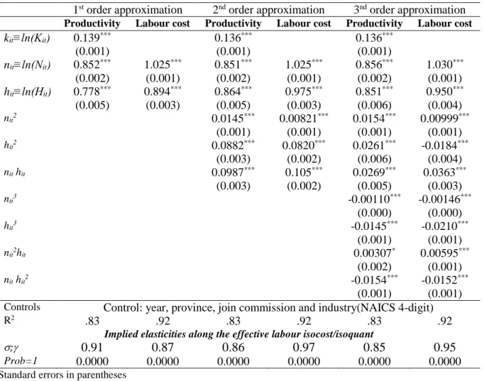
A first set of key results are presented in Table 5. Estimated coefficients using firm-level mean-centred variables21 _{– corresponding to equations [12], [13], but also order 1 simplifications or}

order 3 generalisations – are reported in the upper part of the Table whereas the implied elasticities 𝛾𝛾(nit,hit) [18] σ(nit,hit) [19] along (respectively) the isoquant and the isocost are reported in the lower part of the table. Focusing on the latter, we can see that they are systematically (and statistically significantly) inferior to 1. For instance, the model delivers a value of σ= .80, in line with results of the literature on the elasticity of output to hours (Leslie & Wise, 1980; Anxo & Bigsten, 1989; Cahuc et al., 2014; Cette et al., 2015). The OLS model and FE effects model using first-differenced data (Table 5a, 5b) are presented in the Appendix and deliver estimates qualitatively similar.

In Table 6, we exploit the fact that our data permit replicating the labour cost analysis [using FE-first differences] for three types of employment contracts: full-time (forming the largest part of the total), part-time and interim/temporary. Two interesting results emerge. First, all types of contracts are associated to quasi-fixed labour costs as all estimated 𝛾𝛾 are statistically inferior to 1. Second, conditional on hourly wage elasticity (ε) to be similar across types, fixed costs appear significantly higher for full-time employees: at least 34% compared to 15.4% and 5.4%

21 The mean-centered variables that we use are the original/untransformed ones. Our model writes y(xit)=f(xit)+

ωi+ρit . Mean-centering yit- 𝑦𝑦�i =f(xit)- �������� +ρ𝑓𝑓(𝑥𝑥_{𝚤𝚤𝑖𝑖}) it-𝜌𝜌̅i eliminates (endogenous) fixed effect ωi . But neither f(.)

nor 𝑓𝑓(𝑥𝑥�������� are observed. For f(x_{𝚤𝚤𝑖𝑖}) it), we resort to polynomial approximation. In the case of a 2nd degree

approximation, we have that for value xit expected outcome is given f(xit)≃α + β xit+ γ xit2 . Similarly the

expected outcome value in 𝑥𝑥̅i is given by f(𝑥𝑥̅i) ≃α + β 𝑥𝑥̅i+ γ 𝑥𝑥̅i 2 . Assuming further that 𝑓𝑓(𝑥𝑥��������≃ α + β 𝑥𝑥̅_{𝚤𝚤𝑖𝑖}) i +

14 for part-timers and interims respectively. This result is in line with the model’s prediction that job positions that are associated with higher quasi-fixed costs should be filled with full-time workers whereas part-timers should only be hired when quasi-fixed costs are relatively lower. Results regarding temporary workers should be interpreted with caution as the data for such workers is much weaker: only a small proportion of firms report the presence of temporary workers and the reporting is based on hours invoiced by the interim company.

In Table 7, we explore the varying importance of quasi-fixed labour costs across broadly defined (NACE1) and contrasted industries: manufacturing, retail and accommodation/restaurants. The analysis is done separately for the 3 industries, using FE-first differences. Conditional on hourly wage elasticity (ε) to be uniformly distributed, fixed costs appear to be significantly higher in manufacturing (at least 40%) compared to retail and accommodation/restaurants (26% and 21% respectively). These differences can reflect differences in the labour cost structure between sectors due to for example historically different institutional arrangements and more details on what exactly drives our measure of fixed labour costs are given in section 5. For further results on industry by industry results, see section 3.2 below.

In Table 8, we present the results when endogeneity stems both from fixed effects (unobserved time-invariant firm heterogeneity) and simultaneity (unobserved, final demand-related, short-run shocks that can affect simultaneously outcomes variables and the level of labour inputs).22 To control for that risk we implement the more structural approach developed by Levinsohn & Petrin (2003) and more recently by Ackerberg et al. (2015) (ACF hereafter), which primarily consists of using intermediate inputs (materials and other supplies…) to proxy short-term shocks. Results are qualitatively very similar to the ones reported in previous tables where we control only for fixed effects. Even though this suggests that simultaneity is a relatively benign problem in our data, coefficients in Table 8 are our most robust and thus preferred ones. Referring to Table 8’s ACF results23, the tentative conclusion would be that quasi-fixed labour costs account for at least 23% of total labour costs. As far as we know, this has never been estimated econometrically so far.

More generally, it should be noted for all tables that our contribution resides principally in the correct estimation of elasticities along the isoquant (σ) and the isocost (𝛾𝛾) to be both significantly lower than one. Estimations along the isoquant are not new and should be understood as the demonstration that our database yields results aligned with the existing empirical literature. On the other hand, results regarding the isocost have not be shown before and represent an important contribution to the literature on labour demand. Finally, even though the theoretic model predicts perfect alignment of σ and 𝛾𝛾, our regression models are not built to test such a prediction and the close values we obtain econometrically should only be interpreted as global coherence in our results.

22 For instance, the simultaneity of a negative shock (due to the loss of a major contract) and a reduction of hours worked, causing reverse causality: from productivity drop to hours contraction. Alternatively, focusing on the estimation of the labour cost function, the simultaneity between a positive shock (ex: the landing of a big contract, triggering an overall rise of wages) and a rise of the number of hours worked, also causing a reverse

causality problem [in particular a shock-driven rise of hourly wage elasticity (ε) that may translate into γ being

underestimated].

23 See Vandenberghe (2017) for a full presentation of the LP and ACF proxy-variable idea, and (Vandenberghe et al., 2013) for how it can be combined with fixed-effects.

15

Table 5 – Econometric estimation of the productivity of hours and of the (relative) importance of quasi-fixed labour costs – Fixed effect as mean centring

1st _{order approximation 2}nd _{order approximation 3}nd _{order approximation}

Productivity Labour cost Productivity Labour cost Productivity Labour cost kit≡ln(Kit) 0.0878*** 0.0864*** 0.0853*** (0.001) (0.001) (0.001) nit≡ln(Nit) 0.779*** 0.926*** 0.788*** 0.930*** 0.800*** 0.933*** (0.002) (0.001) (0.002) (0.001) (0.003) (0.002) hit≡ln(Hit) 0.627*** 0.711*** 0.672*** 0.746*** 0.687*** 0.759*** (0.004) (0.003) (0.005) (0.003) (0.005) (0.003) nit2 -0.00159 -0.00973*** -0.00421* -0.00150 (0.001) (0.001) (0.002) (0.001) hit2 0.0830*** 0.0699*** -0.0388*** -0.0678*** (0.003) (0.002) (0.005) (0.003) nit hit 0.0908*** 0.0805*** -0.0344*** -0.0367*** (0.003) (0.002) (0.006) (0.004) nit3 -0.00444*** 0.00159*** (0.001) (0.000) hit3 -0.0270*** -0.0307*** (0.001) (0.001) nit2hit -0.0189*** -0.00997*** (0.002) (0.001) nit hit2 -0.0422*** -0.0412*** (0.002) (0.001)

Controls Control: year, province, join commission and industry(NAICS 4-digit)

R2 _{.83 .92 .83 .92 .83 .92}

Implied elasticities along the effective labour isocost/isoquant

σ;γ 0.80 0.77 0.67 0.75 0.68 0.76

Prob=1 0.0000 0.0000 0.0000 0.0000 0.0000 0.0000

Standard errors in parentheses Source: Bel-first

16

Table 6- Econometric estimation of the (relative) importance of quasi-fixed labour costs. Breakdown by type of contract (full-time, part-time and interim)

FE (first diff.) All types of workers Full-time workers Part-time workers Interim workers nit 0.815*** 0.862*** 0.938*** 0.974*** (0.002) (0.003) (0.003) (0.002) hit 0.642*** 0.657*** 0.845*** 0.946*** (0.003) (0.004) (0.004) (0.005) nit2 0.0392*** 0.0308*** 0.00744*** 0.00388* (0.001) (0.002) (0.002) (0.002) hit2 -0.00771*** 0.00261* -0.0147*** 0.00112 (0.001) (0.001) (0.001) (0.004) nit hit 0.0326*** 0.0378*** -0.00553 -0.00274 (0.002) (0.002) (0.003) (0.005)

Controls Control: year and firm fixed effects

R2 _{.6 .56 .56 .86}

Implied elasticities along the effective labour isocost

γ 0.645 0.660 0.846 0.946

prob=1 0.000 0.000 0.000 0.000

Standard errors in parentheses Source: Bel-first

* _{p < 0.05,} ** _{p < 0.01,} *** _{p < 0.001}

Note that only large firms are required to report information on temporary workers’ hours and cost separately.24

Table 7- Econometric estimation of the (relative) importance of quasi-fixed labour costs. Breakdown by broadly defined industries (Manufacturing, Wholesale and Retail and Accommodation and

Restaurants)

FE (first diff.) All industries Manufacturing Wholesale &

Retail Accommodation & Restaurants nit 0.815*** 0.775*** 0.841*** 0.822*** (0.002) (0.005) (0.005) (0.007) hit 0.642*** 0.594*** 0.732*** 0.780*** (0.003) (0.006) (0.007) (0.009) nit2 0.0392*** 0.0568*** 0.0456*** 0.0185*** (0.001) (0.002) (0.003) (0.003) hit2 -0.00771*** -0.00730*** 0.0169*** -0.00947 (0.001) (0.002) (0.002) (0.007) nit hit 0.0326*** 0.0548*** 0.0644*** 0.00862 (0.002) (0.003) (0.003) (0.007)

Controls Control: year and firm fixed effects

R2 _{.6 .64 .53 .79}

Implied elasticities along the effective labour isocost

γ 0.645 0.596 0.736 0.781

prob=1 0.0000 0.000 0.000 0.000

Standard errors in parentheses Source: Bel-first

* _{p < 0.05,} ** _{p < 0.01,} *** _{p < 0.001}

24 Large firms are firms with more than 100 workers, or firms exceeding 2 of the following thresholds: 50 FTE workers, 7.300.000€ turnover, 3.650.000€ total balance sheet.

17

Table 8 - Econometric estimation of the productivity of hours and of the (relative) importance of quasi-fixed labour costs. Fixed effect as mean centring + accounting for simultaneity bias

LP£ _ACF$

Productivity Labour costs Productivity Labour costs

Nit 0.645*** 0.684*** 0.756*** 0.914***

(0.004) (0.004) (0.006) (0.008)

Hit 0.475*** 0.464*** 0.564*** 0.701***

(0.008) (0.008) (0.063) (0.052)

Controls Year and firm fixed effects [and (log of) capital in productivity equation]

Implied elasticities along the effective labour isocost/isoquant

σ; γ .74 .68 .74 .77

prob=1 0.000 0.000 0.002 0.000

£: Levinsohn-Petrin; $ Ackerberg, Caves & Frazer Cobb-Douglas specification of Q(N,H) and C(N,H)

Standard errors in parentheses Source: Bel-first

* _{p < 0.05,} ** _{p < 0.01,} *** _{p < 0.001}

3.2. Industry-level analysis of the impact of quasi-fixed costs on the demand for hours

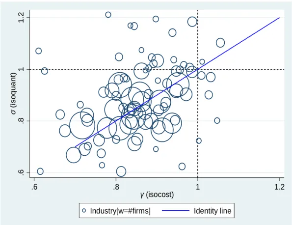
In this section, we derive distinct estimates of 𝛾𝛾(N,H) and σ(N,H) for each of the NACE 3-digit industries in our data set. We first estimate our productivity and labour cost equations separately for each industry25. Results are reported in Table 10 (in the Appendix) and can be visualized on Figure 3. The latter suggests that the two estimates are strongly correlated but not necessarily perfectly aligned. Values of _{𝜎𝜎; 𝛾𝛾}� < 1 hint at the presence of quasi-fixed labour costs whose effect dominates those of longer hours on unit wage (ε≥0). Note that most of the large industries (representing more firms and revealed by the size of the circles on Fig.3) display elasticities that are significantly inferior to 1; an indication of the relative importance of quasi-fixed labour costs.

18 Figure 3- Industry by industry estimation of 𝛾𝛾 and σ

2nd _{order polynomial specification of Q(N,H) and C(N,H)}

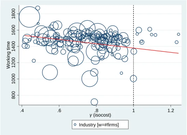
More related to the point at the core of this paper, using these estimates 𝛾𝛾� and 𝜎𝜎� as predictors of (conditional) labour demand equations [11] yields the theoretically expected results (see Table 9, left part). The higher 𝛾𝛾� (i.e. the lower the estimated share of fixed costs), the lower the average annual number of hours (Tab 9, col 3 & Fig 4), and also the higher the share of workers with a part-time contract (Tab 9, col 3 & Fig 5).

Table 9 - Econometric Results – Impact of industry-level elasticity on working hours and prevalence (share) of part-time work contract; using industry by industry estimated 𝜎𝜎�j;𝛾𝛾�j

[FE (first diff.) and 2nd order polynomial specification of Q(N,H) and C(N,H)]

Productivity Labour costs

Working hours Share part-time

contracts

Working hours Share part-time

contracts

𝜎𝜎�j_;𝛾𝛾� j _-0.163*** _0.0848*** _-0.115*** _0.00512***

(0.001) (0.001) (0.001) (0.001)

Controls Year fixed effect,

output (log) Standard errors in parentheses

Source: Bel-first * _{p < 0.05,} ** _{p < 0.01,} *** _{p < 0.001} .6 .8 1 1. 2 σ ( is oq ua nt ) .6 .8 1 1.2 γ (isocost)

19 Figure 4 – Working hours in 2015 as a function of industry-level estimated isocost elasticity

(𝛾𝛾�j

)

Figure 5 – Share of part-time work in 2015 as of industry-level estimated isocost elasticity(𝛾𝛾�j₎

80 0 10 00 12 00 14 00 16 00 18 00 W o rki n g t ime .4 .6 .8 1 1.2 γ (isocost) Industry [w=#firms] 0 .2 .4 .6 .8 Sh a re p a rt -t ime e mp lo yme n t .4 .6 .8 1 1.2 γ (isocost) Industry [w=#firms]

20

4. Robustness checks

4.1. Econometric analysis of worker-level wage data to estimate labour costs.

In this section, we use PIAAC 2012 data26 _{on average gross wage per hour (HC) and hours of}

work per week (H) from the individuals who work as employees in the private, for-profit segment of the economy. By definition, PIAAC aims at delivering comparable international data. It is analysed here with the aim of assess how Belgian quasi-fixed labour costs compare with the situation in other countries. PIAAC contains only individual-level data so there is no way one can replicate the productivity & labour cost analysis of the previous sections. And as in the above sections, the objective is to infer the presence (and the importance) of quasi-fixed labour costs F from the parameters of an econometric models regressing labour cost on hours. As in Section 3.1 we assume that HC(H)=(wH+F)/H= w+F/H. We do not observe unit wage w or fixed labour cost F. But elasticities can be retrieved by the estimation of a linear27 approximation of the log of HC(H) i.e.:

ℎ𝑐𝑐𝑖𝑖𝑖𝑖 ≈ 𝐴𝐴𝑖𝑖+ 𝜙𝜙𝑖𝑖ℎ𝑖𝑖𝑖𝑖 + 𝜆𝜆𝑖𝑖𝜋𝜋𝑖𝑖𝑖𝑖+ 𝜈𝜈𝑖𝑖𝑖𝑖 [22.] where hcik is the (log of) the average gross wage per hour reported by worker i in country k and hik the (log) of number of hours per week the worker declares. Assuming the actual process generating wages is HC= (w+F/H); [ignoring individual and country indices] we have that

𝜕𝜕ℎ𝜕𝜕 𝜕𝜕ℎ

=

=

which is negative [i.e. gross wage per hour go down with hours] if F>0 and if w'(H) is relatively small or null. In the particular case where w'(H) ≈0 [i.e. no or little rise of the wage rate with hours it is immediate to show that δhc/δh = -F/(F+wH) ≈ ϕ. This means that the estimation of [22] delivers coefficients that can be used to estimate the share of quasi-fixed labour costs. Indeed, – ϕ is a lower bound proxy of the importance of quasi-fixed costs.

Of course, the level of hourly gross wage of an individual worker reflects many things that have little to do with the number of working hours. As PIAAC is not a panel, there is no way to resort to fixed effects (FE) to account for unobserved heterogeneity. What we do is to specify πik as a vector of controls comprising many of the determinants of wage: educational attainment, gender, labour market experience, labour market experience squared, occupation (ISCO 2008 2-digit) industry (ISIC 2-digit). We also include the respondent's average test score in literacy, numeracy and problem solving (which turns out to be a key determinant of wage, given Table 10’s results). The hope is that this rather rich set of controls allows for a proper identification of actual gross wage/hours elasticity ϕ, and thus of the (relative) importance of quasi-fixed labour costs.

26 The OECD led Programme for the International Assessment of Adult Competencies (PIAAC)

27 The estimation was conducted using quadratic and cubic approximations. Results were qualitatively similar to that reported hereafter.

21 Results (Appendix, Table 11) clearly hint at the presence of quasi-fixed labour costs. With an estimated ϕ =-.18 for Belgium we may conclude that fixed costs are at least equal to 18% of total gross wage of a typical private- and for-profit economy employee28_{. The figure of 0.18%}

is also very similar to the values estimated using Belgium-only firm-level data in the previous sections. We read PIAAC results as reinforcing the overall plausibility of the firm-level evidence presented above.

4.2. Descriptive/accounting evidence about the share of quasi-fixed labour cost (and their impact on the demand for hours)

Another robustness assessment of our Section 3 econometric estimates of the share of quasi-fixed labour costs comes from the comparison with direct estimates of that share, based on accounting/descriptive data. In general, authors consider both "one-time" fixed costs (i.e. recruitment, training, severance) and "recurrent" fixed labour costs i.e. employer-funded unemployment, medical insurance or retirement plans (social security), remuneration of non-worked days (annual holiday, sick or maternity leave), and other in-kind employee benefits (stocks, cars, phones…).

Summing up these items, several authors report values that are surprisingly close to 20%. Hart (1984), suggests that for both the United States and the United Kingdom it is reasonable to put quasi-fixed labour costs at roughly 20 percent of total cost. For Ehrenberg (2016), the [USA] data suggest that around 19 percent of total compensation (about 60 percent of nonwage costs) is quasi fixed. Martins (2004), in a study for Portugal, estimates quasi-fixed costs at 25 per cent of labour costs, with social security payments are the dominant quasi-fixed cost item.

Finally, there is a small literature that used descriptive estimates of quasi-fixed labour costs as predictor of firms' behaviour. Cutler & Madrian (1998) find that increases in health insurance costs during the 1980s increased the hours of covered workers. Montgomery & Cosgrove (1993) and Buchmueller (1999) show that a smaller proportion of hours are worked by part-time employees in firms offering more generous fringe benefits to full-part-time workers. Finally, Dolfin (2006) uses US data on the cost of recruiting, search, hiring, training, and firing and shows that these increase employee hours ceteris paribus. The results of these studies are consistent with our results in Section 3.2. based on inferred/indirect measures of quasi-fixed labour costs. More generally, they accord with the idea of substitution of hours for workers in response to rising quasi-fixed costs, as predicted by a theory of labour demand.

5. The economic and institutional factors underpinning

quasi-fixed labour cost in the Belgian context

In this final section, we describe what may drive quasi-fixed labour costs in the specific context of Belgium. There is not much to say about 'one-time fixed costs': recruitment, firing/severance and training costs. Like in the case of other advanced economies, these exist in Belgium and are unambiguously "fixed". The singularity of Belgium is that its severance costs -- particularly for white-collar workers -- are very high and may be a significant contributor to Belgium's overall level of quasi-fixed costs. Things are trickier when it comes to "recurrent" quasi-fixed

28 This is slightly below the 20-23% that we got using firm-level data. But remember that PIAAC is only about gross wage whereas Bel-first, firm-level data used in previous section is about total payroll cost (with the possibility that some of elements constituting the differences (employers' social security contributions, taxes, perks) … drive fixed costs upwards).

22 labour costs; which American labour economists traditionally associate to nonwage compensation. Not all components amount to ‘purely’ quasi-fixed costs, as some are directly or indirectly indexed on hours. Only a cautious, case-by-case examination may lead to a definite judgement as to their degree of "fixity".

Strictly speaking, in Belgium all social security contributions (financing the health and unemployment insurances and legal pensions; i.e. the 1st _{pillar) are computed as a percentage} of the gross remuneration, that is itself proportional to the number of hours worked. Therefore, these contributions do a priori not qualify as "fixed". Also, in principle, important mandatory benefits (end-of-year bonus, single and double holiday bonuses) are directly indexed on annual hours of hours. For instance, if the worker has been absent during the year, the amount of her end-of-the-year bonus is reduced pro-rata the number of days of absence. The same logic holds for occupational pensions (the so-called 2nd pillar of the pension system, paid by the employers to top-up legal pensions). Instalments are indexed on salaries, and thus on hours. However, there exist in Belgium many regimes of "assimilation" i.e. days not worked but "assimilated" to days of work and thus remunerated and/or qualifying for social security payments. The most important one is the regime of employer-paid sick leave29_{. But the list also comprises}

maternity/parental leave, educational/training leave, union leave… There is also a regime of "economic unemployment"; i.e. situations of temporary economic recess where workers are sent home but are still paid by the employers. All these "assimilated" days give rise to a sizeable additional labour cost… but which is a priori indexed on hours worked30.

This said, there are, in Belgium many elements of nonwage compensation that are clearly "fixed". Employers must insure each employer against the risk of workplace and home-to-work commuting accident. Whatever the number of hours worked, employees benefit from mandatory, employer-paid, health checks performed on the workplace. More significantly, over the past decades, and mainly for fiscal reasons31, Belgian employers have considerably expanded the use of in-kind benefits. These are quintessentially "fixed". The most significant one is the company car (that can represent up to 20% of a worker's gross remuneration). Other in-kinds comprise home/work travel allowances32_{, mobile phones, laptops and tablets… There}

are many other sources of "fixity" worth mentioning. An example are the relatively strict rules regarding the minimum duration [and pay] for part-time and night-shift work. For part-time, the contract should be for a weekly minimum of 1/3 of the reference full time; with a daily

29 Paid sickness leaves represent a large cost for firms. In fact, in the Belgian system, sickness leave is highly comparable to paid holiday in terms of cost for the firm. The first 30 days of each sick leave are paid for by the employer; and days of absence due to sickness still entitle workers to the associated yearly premium, paid holidays, pension and health insurances, … After 30 consecutive days, the replacement wage is paid for by the social security and the worker may lose some of the perks. On average in Belgium, 50% of employees take at least one day of sick leave per year. Among those, sick leaves last on average 13 days but the average number of days paid by the firm is around 5 days. The percentage of workers taking at least one sick day is similar among blue and white collars, but the average leave length is quite different, 8 days for white collar (5 paid for by the firm), 16 days for blue collar (7 paid for by the firm). The share of workers taking at least one day of sick leave also strongly increases with the size (number of workers) of the firm: from 32% for firms of 1 to 4 workers up to 60% for the largest firms (above 1000 workers).

30 Mathematically, if H1 is the number of hours actually worked and H2 is the number of "assimilated" hours, the

total labour cost writes LC= F+wH1+wH2 = F+w(H1+H2). If H2/H1=α is constant (ex: a probability of

illness...), then the assimilated days are similar to a variable costs i.e. LC= F+w(1+α)H1. There is simply that

the effective wage rate w$_=w(1+α) is inflated pro-rata the typical share of "assimilated" hours.

31 Belgium is characterised by a very large fiscal wedge on labour. One way for companies and workers to reduce payment is to resort to in-kind benefits.

23 minimum of 3 hours. Per-day minima for night-shift workers (> 10 PM) is even stricter33. The point is they are a clear source of non-proportionality between labour costs and hours. Returning to the issue of "assimilated" hours, there are reasons to believe that, in the expression LC=F+w(1+α)H1, α= H2/H1 is probably decreasing with H1. Why? The most obvious case is that of temporary/economic unemployment. It typically intervenes during periods of overall reduction of the number hours worked (i.e. low H1). Also, some "assimilation" regimes (e.g. maternity leave) are more frequent among employees who typically work less hours (women). One unknown feature of Belgium's occupational pensions is the presence of "social" contributions: extra payments by employers aimed at improving the pension capital of the lowest earners; that also often correspond to those working less hours34_{. Finally, it is likely that}

more and more recruitment decisions (at least for white-collars and middle or top managers...) amount to lump-sum commitments: an annual salary (+ benefits) for an indicative number of hours of service; that de facto fluctuate considerably, with no or little implications on the amount received. This increase in lump-sum work contracts emerges mostly for tax avoidance and employee motivation reasons but it should be understood from our work that this phenomenon most probably has strong consequences on working time demand by firms.

6. Concluding remarks

Hours worked tend to vary across individuals, but also – on average – across firms, and even within firm over time. Why? Over the past decades, most economists have privileged the idea that shorter versus longer hours (leaving labour-market regulations aside) had primarily to do with the preferences of individuals. In this work, echoing Pencavel (2016)'s question of "Whose Preferences Are Revealed in Hours of Works?", we explore the role of employers' preferences for working time; and in particular the role of quasi-fixed labour costs. By quasi-fixed labour costs, we mean any expense that are associated with employing a worker but are independent of his/her hours of work (such as the costs of fringe benefits, sickness leaves, hiring and training new workers, firing workers35 …).

We consider a setup where firms decide simultaneously on working hours and the number of workers. We find that despite an obvious productivity gain from reducing working hours, firms facing large quasi-fixed labour costs choose a higher level of hours to cover such quasi-fixed labour costs.

We estimate that increasing hours by one percent would only increase the output (value-added) by 0.8 percent, thus in line with the hypothesis of decreasing marginal return to working hours, and that imperfect substitutability between hours and workers in the production process. What is more – and to our knowledge this is a novelty – we able to retrieve the relative share of quasi-fixed labour costs: 20 to 23 percent of a worker’s cost could be independent from hours. These econometric results suggest that the typical for-profit firm located in Belgium face financial incentives to raise hours beyond the point where the average productivity starts declining. They

33 Min{6 hours, typical day-shift number of hours}.

34 Formally, the consequences of H2/H1 being non-constant are that the average labour cost per hour becomes

LC/H1 = F/ H1 + w(1+α(H1)) and the derivative with respect to hours worked d(LC/H1)/dH1=-F/H12 +

wdα(H1)dH1. So, if dα(H1)dH1<0, the deflating effect of longer hours of work H1 is magnified. Formally, the

consequences of H2/H1 being non-constant are that the average labour cost per hour becomes LC/H1 = F/ H1

+ w(1+α(H1)) and the derivative with respect to hours worked d(LC/H1)/dH1=-F/H12+ wdα(H1)dH1. So if

dα(H1)dH1<0, the deflating effect of longer hours of work H1 is magnified.

24 explain why ceteris paribus some industries (i.e. those with higher quasi-fixed labour costs) are characterised by longer hours and a lower propensity to employ people on a part-time basis. They could also explain why some firms, or some industries oppose reducing working hours, even in the absence of compensatory36 _{rise of hourly wages.}

In short, when it comes to working time policies – often touted as crucial to accommodate the varying needs and desires of postmodern individuals – firms' preferences and their determinants should not be ignored. As long as firm have some power to determine the hours of work of their employee, taking into account their preferences will allow policy makers to better understand why some sectors more than others might oppose working-time reduction policies. Also, reducing or eliminating quasi-fixed labour costs can be an additional lever to increase the opportunities of gradual retirement for the swelling ranks of older workers.

36 By 'compensatory' rise of hourly wages we refer to what is needed to meet demands of reduced working without any loss of total wage.

25

References

Ackerberg, D. A., Caves, K. and Frazer, G. (2015). Identification Properties of Recent Production Function Estimators, Econometrica, 83, pp. 2411–2451.

Altonji, J.G., Paxson, C.H., 1986. Job characteristics and hours of work. In: Ehrenberg, R.G. (Ed.), Research in Labor Economics, vol. 8. Part A. Westview Press, Greenwich, pp. 1–55. Altonji, J.G., Paxson, C.H., 1988. Labor supply preferences, hours constraints and hours-wage tradeoffs. Journal of Labor Economics 6, 254–276.

Altonji, J.G., Paxson, C.H., 1992. Labor supply, hours constraints and job mobility. Journal of Human Resources 27 (2), 256–278.

Anxo, D. and Bigsten, A. (1989). Working hours and productivity in Swedish manufacturing. The Scandinavian Journal of Economics, 91(3):613– 619.

Barzel, Y. (1973). The determination of daily hours and wages. The Quarterly Journal of Economics, 87(2):220–238.

Buchmueller, T. (1999), Fringe benefits and the demand for part-time workers, Applied Economics, 31, 551–63.

Bryan, M. L. (2007). Workers, workplaces and working hours. British Journal of Industrial Relations, 45(4):735–759.

Cahuc, P., Carcillo, S., Zylberberg, A., and McCuaig, W. (2014). Labor economics. MIT press.

Cette, G., Dromel, N., Lecat, R., and Paret, A.-C. (2015). Production factor returns: the role of factor utilization. Review of Economics and Statistics, 97(1):134–143.

Collewet, M. and Sauermann J. (2017). Working Hours and Productivity, IZA Discussion Papers No 10722, Institute for the Study of Labor.

Cutler, D. and Madrian, B. (1998) Labor market response to rising health insurance costs: evidence on hours worked, RAND Journal of Economics, 29, 509–30

Dixon, R. and Freebairn, J. (2009). Models of labour services and estimates of Australian productivity, Australian Economic Review, 42(2):131–142.

Dixon, R., Freebairn, J., and Lim, G. C. (2005). An employment equation for Australia. Economic Record, 81(254):204–214.

Dolfin, Sarah, (2006), An examination of firms' employment costs, Applied Economics, 38, issue 8, p. 861-878.

Donaldson, D. and Eaton, C. (1984). Person-specific costs of production: hours of work, rates of pay, labour contracts. Canadian Journal of Economics, pages 441–449.

Ehrenberg, R.G. (2016), Modern Labor Economics: Theory and Public Policy, Routledge, Abingdon, Oxon; New York (12th edition).

Feldstein, M. (1976). Temporary layoffs in the theory of unemployment. Journal of political economy, 84(5):937–957.

Feldstein, M. S. (1967). Specification of the labour input in the aggregate production function. The Review of Economic Studies, 34(4):375–386.