AM-FM signal Analysis by Teager Huang Transform: application to underwater acoustics

HAL Id: tel-00818032

https://tel.archives-ouvertes.fr/tel-00818032

Submitted on 26 Apr 2013

HAL is a multi-disciplinary open access

archive for the deposit and dissemination of sci-entific research documents, whether they are pub-lished or not. The documents may come from teaching and research institutions in France or abroad, or from public or private research centers.

L’archive ouverte pluridisciplinaire HAL, est destinée au dépôt et à la diffusion de documents scientifiques de niveau recherche, publiés ou non, émanant des établissements d’enseignement et de recherche français ou étrangers, des laboratoires publics ou privés.

Abdelkhalek Bouchikhi

To cite this version:

Abdelkhalek Bouchikhi. AM-FM signal Analysis by Teager Huang Transform: application to under-water acoustics. Signal and Image Processing. Université Rennes 1, 2010. English. �tel-00818032�

THÈSE / UNIVERSITÉ DE RENNES 1

uqwu"ng"uegcw"fg"nÓWpkxgtukvfi"Gwtqrfigppg"fg"Dtgvcipg

pour le grade de

FQEVGWT"FG"NÓWPKXGTUKV¡"FG"TGPPGU"3

Mention : TRAITEMENT DU SIGNAL et TELECOMMUNICATIONS

Ecole doctorale MATISSE

Présentée par

Abdelkhalek BOUCHIKHI

Pré

rctfig" "nÓ

IRENav, EA 3634, Ecole Navale

(SPM)

Analyse des Signaux

AM-FM par

Transformation de

Huang-Teager :

Application à

nÓ

acoustique

sous-marine

devant le jury composé de :

Nadine MARTIN

DR CNRS, Univ. Grenoble / Rapporteur

Messaoud BENIDIR

Professeur, Paris-Sud / Rapporteur

Jean Marc BOUCHER

Professeur, Télécom Bretagne / Examinateur

Xavier NEYT

Professor, Ecole Royale Militaire / Examinateur

Ali KHENCHAF

Professeur, ENSIETA / Directeur de thèse

Abdel-Ouahab BOUDRAA

MCF, HdR, Ecole Navale / Encadrant

Jean Christophe CEXUS

Je tiens à remercier en premier lieu Abdel-Ouahab Boudraa, mon encadrant de thèse. Sans son enthousiasme et son amical soutien, je ne sais si cette thèse sur la théma-tique de l’analyse des signaux AM-FM par l’EMD aurait été menée à son terme, "Rabi yarham waldik, abdel-ouahab". Je remercie aussi mon directeur de thèse Ali Khenchaf, Professeur des Universités à ENSTA Bretagne, pour sa disponibilité mal-gré son emploi de temps assez chargé. Ses conseils m’étaient toujours indispensables. Je remercie également ici avec la plus grande sincérité les personnes qui ont participé de près ou de loin à ce travail de thèse.

Je tiens tout d’abord à remercier les membres du jury qui m’ont fait l’honneur d’évaluer ce travail. Je remercie Jean-Marc Boucher, Professeur à Télécom Bretagne, d’avoir apporté son regard personnel et de m’avoir fait le plaisir de présider le jury. Je remercie Madame Nadine Martin, Directrice de Recherche au CNRS (GIBSA-lab), et Messaoud Benidir, Professeur des Universités à Paris 11, d’avoir pris le temps de soigneusement étudier ce manuscrit et de le rapporter en me faisant part de leurs nombreuses questions et recommandations. Je remercie également Xavier Neyt, Professeur à l’Ecole Royale Militaire (Bruxelles), d’avoir apporter un regard critique sur le contenu scientifique de cette thèse. Je remercie beaucoup Jean Christophe Cexus, Enseignant-Chercheur à ENSTA Bretagne, d’avoir accepté de participer à ce jury et surtout d’avoir apporté son soutien à mes travaux de recherche, ça m’a fait beaucoup de plaisir de travailler avec toi " J. Christophe Sénior ! ". Je remercie également Laurent Guillon, Maître de Conférences à l’Ecole Navale, Docteur El-hadji Diop, Gérard Maze, Professeur des Universités à l’Université du Havre, et le Docteur John Fawcett, Chercheur au DRDC Atlantic (Canada), pour les discussions enrichissantes et les nombreuses remarques qui ont participé à l’avancement de ce travail de recherche. Mes remerciements vont aussi au personnel de l’Institut de Recherche de l’Ecole Navale (IRENav) en particulier, Jacques André Astolfi, Maître de Conférences à l’Ecole Navale, Christophe Claramunt, directeur de l’IRENav, ainsi que Radjesvarane Alexandre, Professeur des Universités à l’Ecole Navale, pour leurs soutiens. Je remercie également l’équipe du laboratoire d’Extraction et Exploitation de l’Information en Environnements Incertains (E3I2) de l’ENSIETA et en partic-ulier Mme Annick Billon-Coat pour son aide.

Je tiens à remercier ici mes collèges à l’équipe RESO de l’ENIB, en particulier Maîtres de Conférences Abdesslam Benzinou, Yan Boucher et Docteur Kamal

Rozenn, Kais, Samuel et Louay. Je tiens également à remercier ici mon ami Sobhi, "Rabi ybarek Fik" et tout les Doctorants et Docteurs de l’IRENav sans que j’oublie personne, pour les inoubliables repas des doctorants et les sorties de cohésions, c’étaient des moments vraiment agréables. Je tiens aussi à remercier mes collègues de travail de l’Ecole Navale: département des langues, formation militaire, et en particulier tout le personnel du département des CENOE.

Finalement, il me reste à remercier mes parents, ma femme, Assia, mes trois soeurs, mes frères et mes amis en Algérie, ici en France et partout dans le monde à qui je dois la curiosité qui m’a amené jusqu’ici, et dont le soutien m’a été toujours précieux, "Rabi yhfadkom".

Contents 1 List of Figures 5 List of Tables 10 Abbreviations 12 List of publications 13 Résumé étendu 16 Introduction 22 I Time-frequency representations 28 I.1 Introduction . . . 29

I.2 Fourier transform . . . 29

I.3 Short-Time Fourier Transform . . . 30

I.4 Wavelet Transform . . . 31

I.5 Wigner-Ville Distribution . . . 32

I.5.1 The cross-term issue . . . 32

I.6 Reassigned TF Distributions . . . 32

I.7 Summary . . . 33

II Empirical Mode Decomposition 36 II.1 Introduction . . . 38

II.2 Empirical Mode Decomposition . . . 39

II.2.1 Sifting process . . . 40

II.2.2 Illustrative example . . . 41

II.3 Some aspects of the EMD . . . 45

II.3.1 IMF criteria . . . 45

II.3.2 Number of sifts . . . 45

II.3.3 Number of IMFs . . . 46

II.3.4 Sampling and mode mixing issues . . . 46

II.3.5 Orthogonality . . . 47

II.3.6 Bivariate EMD . . . 47

II.3.7 Ensemble EMD . . . 47

II.3.8 A PDE for sifting process . . . 48

II.4 Smooth B-spline interpolation of IMF . . . 48

II.4.1 Polynomial spline signal . . . 49

II.4.2 Noise reduction . . . 52

II.4.3 Forced oscillatory motion . . . 56

II.5 Summary . . . 56

III Instantaneous frequencies and amplitudes tracking 62 III.1 Introduction . . . 63

III.2 Multicomponent AM-FM Signal Model . . . 63

III.3 ESA or HT ? . . . 65

III.4 HT demodulation . . . 66

III.5 TKEO . . . 67

III.5.1 Discrete energy demodulation . . . 68

III.5.1.1 DESA-1a . . . 69

III.5.1.2 DESA-1 . . . 69

III.5.1.3 DESA-2 . . . 70

III.5.2 Continue energy demodulation . . . 70

III.5.2.1 Demodulation by exact splines . . . 71

III.7 Summary . . . 83

IV Teager Huang Transform 86 IV.1 Introduction . . . 87

IV.2 Teager-Huang Transform . . . 87

IV.3 Teager-Kaiser spectrum . . . 88

IV.3.1 TKS generation . . . 91

IV.4 Results and discussions . . . 92

IV.4.1 Example 1: Hyperbolic frequencies law . . . 92

IV.4.2 Example 2: Monocomponent FM signal . . . 96

IV.5 Conclusions . . . 98

V Teager Huang Hough Transform 102 V.1 Introduction . . . 103

V.2 Hough-Transform . . . 103

V.3 THT and Hough-Transform: THHT . . . 104

V.4 Detection in noise free environment . . . 106

V.4.1 Results . . . 106

V.5 Detection in noisy environment . . . 109

V.5.1 EMD denoising . . . 109

V.5.2 Results . . . 113

V.6 Conclusions . . . 122

VI Application to underwater acoustics 124 VI.1 Introduction . . . 125

VI.2 IMFs versus physical modes . . . 125

VI.2.1 Physical Modes for a spherical shell . . . 126

VI.2.2 IMFs . . . 128

VI.3 Comparison and discussion . . . 131

VI.4 Backscattering signal analysis . . . 133

A Analysis of white gaussian Noise by EMD 148

B The first derivatives of IMF in B-Spline space 154

C Determinant for an empty shell 158

I.1 Jean Baptiste Joseph Fourier. 21 March 1768 Auxerre, Yonne, France [36] . . . 29 II.1 Initialization of the sifting process for s(t), envelope mean detection

(red line) and the first sift of IMF1. Over- and undershoots are indi-cated by arrows. . . 42 II.2 Extraction of the 5 Hz component from s(t) at first iteration. The

local mean envelope is null (red line) and the component contain an acceptable number of extremas. . . 43 II.3 Extraction of the second candidate IMF from s(t). Envelope mean

detection (red line). . . 43 II.4 Extraction of the third candidate IMF from s(t). Envelope mean

detection (red line). . . 44 II.5 Extraction of the third candidate IMF from s(t). Envelope mean

detection (red line). . . 44 II.6 IMFs extracted from signal given in (cf, Eq. II.2.2). The two

com-ponents of frequencies 5 Hz and 1 Hz correspond to IMF1 et IMF2, respectively. . . 45 II.7 EMD-RBS diagram. The modified EMD is distinguished from the

coventional EMD on integrating the smooth B-splines, or Regularized B-splines (RBS) interpolation instead of the cubic splines interpola-tion. Also as in [15] we use the acronym EMD-RBS to refer to the modified EMD. . . 50

II.9 Extracted IMFs by EMD from noisy signal s(t) (SNR=0dB). The conventional EMD failed to extract directly the 5Hz sinusoid. For getting a smooth version of the sinusoidal signal one must add the

IMF 5, the IMF 6 and part of the IMFs 4 and 7. . . 53

II.10 Extracted IMFs by EEMD from noisy signal s(t) (SNR=0dB). The sum of IMF 4, 5 and 6 give a noisy version of the sinusoidal signal but not the original one. . . 54

II.11 Extracted IMFs by EMD-RBS of the noisy signal s(t) (SNR=0 dB). The 5Hz tone is extracted successfully, it corresponds to IMF number 2. . . 55

II.12 variation of the parameter λ . . . 56

II.13 Signal generated by an hydrodynamical system. . . 57

II.14 Extracted IMFs by conventional EMD from hydrodynamical mea-sured signal. In top square IMF1 to IMF5. The square of middle, IMF6 to IMF10 and last one contain remainder IMFs and the residue. 58 II.15 Extracted IMFs by EMD-RBS from hydrodynamical measured signal. In top square, IMF1 to IMF4. The square of middle, IMF5 to IMF8 and last one contain remainder IMFs and the residue. The number of IMFs in the present figure is less than the previous figure. . . 59

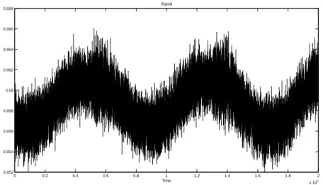
III.1 Two AM-FM components (M = 2) . . . 64

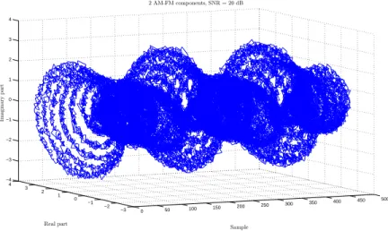
III.2 AS of the two AM-FM components, this representation shows in 3D the complex form of the signal, with their imaginary part and real part. The horizontal axis contain the samples points position. We note that a projection of this signal in the plane (Real part-sample) give the real signal, figure (III.1) . . . 67

III.3 Decomposition of the noisy AM-FM signal, s(t), (SNR=20 dB) with EMD . . . 74

III.4 Decomposition of the noisy AM-FM signal, s(t), (SNR=20 dB) with modified EMD . . . 74

III.5 IAs estimation of noise free signal, s(t), by EMD-ESA-BS . . . 75

III.6 IFs estimation of noise free signal, s(t), by EMD-ESA-BS . . . 76

III.7 IA estimation of signal s(t) (SNR= 20dB) by EMD-ESA-BS . . . 77

III.8 IA estimation of signal s(t) (SNR= 20dB) by EMD-ESA-RBS . . . . 77

III.10IF estimation of signal s(t) (SNR= 20dB) by EMD-ESA-RBS . . . . 78

III.11IA estimation of signal s(t) (SNR= 20dB) by EMD-HT . . . 78

III.12IA estimation of signal s(t) (SNR= 20dB) by EMD-DESA1 . . . 79

III.13IA estimation of signal s(t) (SNR= 20dB) by EMD-DESA1a . . . 79

III.14IA estimation of signal s(t) (SNR= 20dB) by EMD-DESA2 . . . 80

III.15IF estimation of signal s(t) (SNR= 20dB) by EMD-HT . . . 80

III.16IF estimation of signal s(t) (SNR= 20dB) by EMD-DESA1 . . . 80

III.17IF estimation of signal s(t) (SNR= 20dB) by EMD-DESA1a . . . 81

III.18IF estimation of signal s(t) (SNR= 20dB) by EMD-DESA2 . . . 81

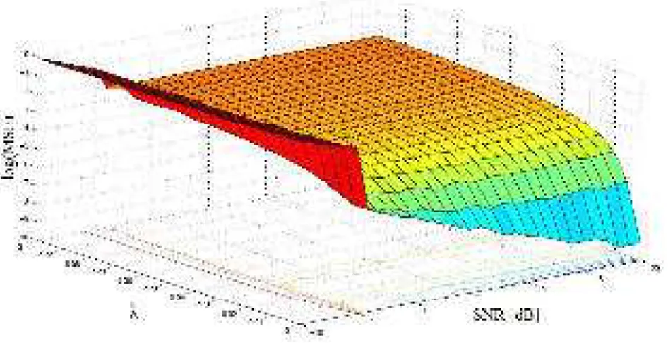
III.19MSE as function of input SNR for different IF estimations of signal s2(t) . . . 82

III.20MSE as function of input SNR for different IA estimations of signal s2(t) . . . 82

IV.1 IFs and IAs estimating by EMD-ESA . . . 88

IV.2 (a) On top a sinusoidal signal, on bottom the corresponding Fourier spec-trum and mean marginal TKS in black and red colors, respectively. (b) THT (EMD-ESA) of the signal. . . 90

IV.3 TFRs of the signal s1(t). (a) Spectrogram with Length of window (Lw = 64), number of overlaps samples in each segment of signal (N ov = 32) and number of frequency points (N f f t = 1024) (c) Spectrogram (Lw = 256, N ov= 64, N f f t = 1024) (d) Scalogram performed by Daubechies wavelet (db2) and in scales S = [1 : 64] (d) Scalogram (Morlet, S = [1 : 64]). The red dashed line corresponds to the real frequency law. . . 93

IV.4 TFRs of the signal s1(t). (a) WVD. (b) SPWVD. (c) RSPWVD. The red dashed line corresponds to the real frequency law . . . 94

IV.5 Decomposition of the signal s1(t) by EMD, the signal is plotted in the first row, the IMF1 to IMF8 correspond to the rows 1 to 8, re-spectively. The last one is the residue. . . 95

IV.6 TFRs of the signal s1(t)., (a) EMD-HT. (b) EMD-ESA. The red dashed line correspond to the real frequency law . . . 96

IV.7 Spectrum analysis of s2(t), (a) Spectrogram. (c) Scalogram. (d) SPWVD (e). RSPWVD (a) EMD-HT. (c) EMD-ESA. The red dashed line corresponds to the real frequency law . . . 97

V.1 Illustration of Hough transform . . . 104

V.2 Block diagram of the THHT. . . 106

V.3 Ideal TFR of the free noise signal x1(t). . . 107

V.4 Components tracking in THT plane of x1(t) . . . 108

V.5 THHT applied to x1(t). . . 109

V.6 Components tracking in WVD plane of x1(t) . . . 110

V.7 WVD-HgT applied to x1(t). . . 111

V.8 Components tracking in SPWVD plane of x1(t) . . . 112

V.9 Ideal TFR of the free noise signal x2(t). . . 113

V.10 Components tracking in THT plane of x2(t) . . . 114

V.11 Components tracking in SPWVD plane of x2(t) . . . 115

V.12 Block diagram of the EMDSG . . . 116

V.13 Ideal TFR of noisy signal x2(t) (30dB). . . 116

V.14 WVD and THT of x2(t). . . 117

V.15 WVD-HgT applied to x2(t). . . 117

V.16 WVD-HgT applied to x2(t). . . 118

V.17 IF estimation (red) with WVD-HgT (on the left) and THHT (on the right) of x2(t). . . 118

V.18 Estimation of β0 . . . 119

V.19 Estimation of ν0 . . . 119

V.20 Components tracking in THT plane of x3(t) (SNR=7dB) . . . 120

V.21 Components tracking in SPWVD plane of x3(t) (SNR=7dB) . . . 121

VI.1 Scattering geometry. This cartoon depicts a plane wave, traveling in the z direction, incident upon a fluid sphere (radius a, density ρ1 and sound velocities cl ct), entrained in a second fluid (density ρ, sound speed c). For simplicity, the scattered waves are shown as spherical, which they are in time, although not generally in phase and amplitude. In the forward region, the scattered field and incident field interfere, and may produce a shadow [47]. . . 125

VI.2 225 kHz echo signal from a spherical shell of radii ratio equal to 0.96. 126 VI.3 Geometry of the scattering calculation. The sphere is centered on the z axis of the plan wave. . . 127

VI.4 On top, filtered time signal (the specular echo is replaced by zeros). The signal is reconstructed from the associated time series of the IMRs of the spherical shell(b/a = 0.94). On bottom, resonance spectrum . . 128 VI.5 Associated time series of the IMRs of a spherical shell, modes 1-10 . . 129 VI.6 IMFs 1-10 extracted from the backscattering signal from a spherical

shell. . . 130 VI.7 PSDs of IMRs . . . 131 VI.8 PSDs of the IMFs . . . 131 VI.9 superposition of PSDs of the IMRs, IMF1 and IMF2 dark and green

dashed lines respectively . . . 132 VI.10(a) Signal and FFT of signal 1. (b) Spectrogram. (c) Scalogram. (d)

SPWVD. (e) HHT. (f) THT. . . 135 VI.11(a) Signal and FFT of signal 2. (b) Spectrogram. (c) Scalogram. (d)

SPWVD. (e) HHT. (d) THT. . . 136 VI.12(a) Signal and FFT of signal 3. (b) Spectrogram. (c) Scalogram. (d)

SPWVD. (e) HHT. (d) THT. (g) Zooming on HHT, (h) Zooming on THT ([1.5, 1.55] ms). . . 138 VI.13(a) Signal and FFT of signal 4. (b) Spectrogram. (c) Scalogram. (d)

SPWVD. (e) HHT. (d) THT. (g) Zooming on HHT, (h) Zooming on THT ([1.5, 1.55] ms). . . 140 VI.14(a) Signal and FFT of signal 5. (b) Spectrogram. (c) Scalogram. (d)

SPWVD. (e) HHT. (d) THT. (g) Zooming on HHT, (h) Zooming on THT ([1.5, 1.55] ms). . . 142 A.1 IMF power spectra in the case of White Gaussian Noise. The

spec-trum densities (PSD) is plotted as a function of the logarithm of the period for IMFs 1 to 7. The spectral estimates have been computed on the basis of 5000 independent sample paths of 4096 data points . . 149 A.2 IMF power spectra in the case of White Gaussian Noise. The

spec-trum densities (PSD) is plotted as a function of the logarithm of the periode for IMFs 1 to 7. The spectral estimtes have been computed on the basis of 5000 independent sample paths of 4096 data points . . 152 A.3 Histograms of IMFs from 2 to 7 for a WGN sample with 4096 data

points.The superimposed black lines are the Gaussian fits for each IMF, except IMF3 . . . 153

II.1 Sifting process . . . 41 III.1 Mean Square Error between estimated IFs and real ones for the noise

free signal. . . 76 IV.1 Proprieties comparison of Fourier analysis, TFRs of Cohen class and

THT. . . 100 VI.1 Statistical parameters of the IMRs. . . 131 VI.2 Statistical parameters of the IMFs. Because the amplitudes of

IMF8-10 are very small the values of the statistical parameters are consid-ered null with the fixed precision . . . 132

AF Ambiguity Function

AM Amplitude Modulation

AS Analytical Signal

DESA Discrete Energy Separation Algorithm

EEMD Ensemble Empirical Mode Decomposition

EMD Empirical Mode Decomposition

ESA Energy Separation Algorithm

FM Frequency Modulation

FT Fourier Transform

FFT Fast Fourier Transform

HHT Hilbert Huang Transform

HT Hilbert Transform

IMF Intrinsic Mode Function

IMR Isolated Modal Resonance

IA Instantaneous Amplitude

IF Instantaneous Frequency

LFM Linear Frequency Modulated

LS Least Squares

ML Maximum Likelihood

MSE Mean Square Error

PDE Partial Differential Equation

PSD Power Spectral Densities

QTFR Quadratic Time Frequency Representation

RADAR RAdio Detection And Ranging

RBS Regularized B-Spline

RSPWVD Reassigned Smooth Pseudo Wigner-Ville Distribution

SD Standard Deviation

SNR Signal to Noise Ratio

SONAR SOund Navigation And Ranging

SPWVD Smooth Pseudo Wigner-Ville Distribution

STFT Short Time Fourier Transform

SG Savitzky-Golay

TF Time Frequency

TFR Time Frequency Representation

THT Teager-Huang Transform

THHT Teager-Huang-Hough Transform

TKEO Teager-Kaiser Energy Operator

TKS Teager-Kaiser Spectrum

WT Wavelet Transform

International Journal Papers :

[1] A. Bouchikhi and A.O. Boudraa, "Multicomponent AM-FM signals analysis based on EMD-B-Splines ESA", Signal Processing (submitted).

[2] A. Bouchikhi, J.C. Cexus and A.O. Boudraa, "A combined Teager-Huang and Hough transforms for LFM signals detection", Signal Processing. (submitted). [3] A.O. Boudraa. J.C. Cexus and A. Bouchikhi, "Time-frequency representation of multicomponent AM-FM signals by Teager-Huang transform", IEEE Trans.

Instrum. Meas. (submitted).

[4] J.C. Cexus, A.O. Boudraa , A. Bouchikhi, et A. Khenchaf, "Analyse des échos de cibles Sonar par transformation de Huang-Teager (THT)", Traitement du Signal, vol. 24, no. 1-2, pp. 119-129, 2008.

[5] K. Khaldi, A.O. Boudraa, A. Bouchikhi and M. Turki-Hadj Alouane, "Speech enhancement via EMD", EURASIP Journal on Advances in Signal Processing, vol. 2008, Article ID 873204, 8 pages, 2008.

International Conference Papers :

[1] A. Bouchikhi, A.O. Boudraa, G.Maze, "Analysis of acoustics signals echos from cylindrical elastic shells by HHT and THT", Proc. International Conference in

Un-derwater Measurements, pp 1455-1460, Nafplion, Greece, 2009.

[2] A. Bouchikhi, A.O. Boudraa, S. Benramdane and E.H.S. Diop, "Empirical mode decomposition and some operators to estimate instantaneous frequency: A comparative study", Proc. IEEE ISCCSP, pp. 608-613, Malta,2008.

[3] K. Khaldi, A.O. Boudraa, A. Bouchkhi, M. Turki-Hadj Alouane and E.H.S. Diop, "Speech signal noise reduction by EMD", Proc. IEEE ISCCSP, pp. 1155-1158, Malta, 2008.

thresholding", Proc. IEEE ISC-CSP, pp. 1086-1090, Malta, 2008.

[5] A.O. Boudraa, T. Chonavel, J.C. Cexus, S. Benramdane and A. Bouchikhi, "On the detection of transient signals using cross-Psi-B-energy operator", Proc. IEEE

IS-CCSP, pp. 1445-1449, Malta, 2008.

[6] E.H.S. Diop, A.O. Boudraa and A. Bouchikhi, "An improved image demodula-tion algorithm based on Teager-Kaiser operator", Proc. IEEE ISCCSP, pp. 876-881, Malta, 2008.

[7] J.C. Cexus, A.O. Boudraa and A. Bouchikhi, "A combined Teager-Kaiser and Hough transforms for LFM signals detection", Proc. IEEE ISCCSP, 5 pages, Li-massol, Cyprus, 2010.

[8] J.C. Cexus, A.O. Boudraa et A. Bouchikhi, "THT et transformation de Hough pour la détection de modulations linéaires de fréquence", GRETSI, 4 pages, 2009, Dijon, France.

[9] A. Bouchikhi et A.O. Boudraa, "Estimation des FIs d’un signal multi-composantes par décomposition modale empirique et une version B-splines de l’opérateur d’énergie de Teager-Kaiser", GRETSI, pp. 817-820, Troyes, France, 2007. [10] A.O. Boudraa, E.H.S. Diop, F. Salzenstein, A. Bouchikhi, "Seuillage d’images basé sur l’opérateur de Teager-Kaiser", GRETSI, pp. 885-888, Troyes, France, 2007.

Les signaux issus des phénomènes physiques sont en général de nature non-stationnaire et dans certains cas ils sont également formés de plusieurs composants fréquentielles (multi-composante). On peut citer comme exemples de signaux non-stationnaires, les signaux, Radar, Sonar, de Parole, sismique ou biomédicaux [12]. Les Représentations Temps-Fréquence (RTF) sont des transformations conjointes forment le cadre idéal pour l’analyse et le traitement de tels signaux. Les RTF de la classe de Cohen constituent un outil puissant pour l’analyse des signaux non-stationnaires. La nature bilinéaire des RTF introduit des interférences (termes croisés) qui nuit à la lisibilité de ces dernières. Le lissage temps-fréquence per-met de réduire ces interférences des RTF, mais certaines de leurs propriétés telles que les marginales ne seront plus vérifiées. Par ailleurs la plupart des RTF sont liées au noyau de Fourier et par conséquent auront intrinsèquement plus ou moins les mêmes limites que la transformée de Fourier. De plus aussi bien les RTF de la classe de Cohen que la transformée en ondelettes nécessitent la connaissance d’un noyau ou d’une fonction de base. Or, il n’existe pas de noyau universel pour représenter tous les signaux. L’idéal est de trouver une décomposition qui s’adapte à chaque signal, sans informations a priori et qui permette une description temps-fréquence. Une solution à ce problème a été proposée par Huang et al. [64] en introduisant la décomposition modale empirique (EMD pour Empirical Mode De-composition). Cette décomposition est entièrement pilotée par les données et la RTF associée obtenue par Transformation d’Hilbert (TH) [12] ou l’algorithme de séparation d’énergie (ESA pour Energy Separation Algorithm) [83] ne présente pas d’interférences. L’EMD est dédiée à l’analyse de signaux non-stationnaires issus ou non de systèmes linéaires. La décomposition d’un signal par EMD produit des com-posantes qui sont des formes d’ondes oscillantes potentiellement non harmoniques dont les caractéristiques (fréquence, amplitude) varient au cours du temps. Ces composantes oscillantes modulées en amplitude (AM) et en fréquence (FM) sont

appelées modes empiriques ou IMFs (pour Intrinsic Mode Functions) : s(t) = N X j=1 IMFj(t) + rN(t), (1)

où N est le nombre d’IMFs et rN(t) est le résidu de la décomposition.

L’EMD est définie par la sortie d’un algorithme appelé processus de tamisage. Dans cette thèse on explore les potentialités de cette méthode en analyse temps-fréquence pour l’estimation d’attributs important tels que l’Amplitude Instantanée (AI) et la Fréquence Instantanée (FI) ou la détection de Modulations Linéaires de Fréquence (MLF) dans le plan temps-fréquence. L’apport de l’EMD est illustré par une application à l’Acoustique Sous-Marine (ASM) ou les signaux sont de nature non-stationnaire.

Nous rappelons dans un premier temps l’intérêt de la représentation fréquen-tielle d’un signal et de la nécessité de l’analyse temps-fréquence dans le cas non-stationnaire. Nous mettons l’accent sur les limites des Représentations Temps-Fréquence (RTF) et le besoin d’un nouveau cadre de description des signaux s’affranchissant de la contrainte du noyau de décomposition et supprimant les termes d’interférences.

Dans un deuxième temps, nous nous penchons sur l’outil EMD et ses variantes. Nous mettons en avant les problématiques inhérentes au tamisage telles que les conditions d’une IMF, l’échantillonnage, l’interpolation des enveloppes du signal à décomposer, la condition d’orthogonalité des modes ou le critère d’arrêt. La version conventionnelle de l’EMD utilise la famille des B-splines [109] pour l’interpolation des enveloppes de maxima et de minima du signal [64]. Les modes ainsi extraits sont des sommes d’interpolations [14],[109]:

IMFn j(t) = X l∈Z cj[l] βjn(t − l) (2) où βn

k(t) est la B-spline centrale de degré n [99] et cj[k] les coefficients du modèle.

Une propriété intéressante des fonctions B-splines est liée à leur support compact, ce qui limite la propagation des erreurs d’approximation d’un intervalle ("box") à l’autre. Cela étant, les enveloppes basées sur les fonctions B-splines ne sont pas assez robustes en présence de bruit car la contrainte d’interpolation est trop forte [15]. Une des conséquence de l’interpolation rigide est la génération d’IMFs artificielles. Dans ce cas, la solution est donc de s’orienter vers une courbe d’approximation des données

et non plus d’interpolation: E = ∞ X l=−∞ (IMFn j(l) − hnj(l))2+ λ Z _∂r_hn j(t) ∂tr !2 dt (3)

où λ est une constante de régularisation, hn

j(l) est le modèle et IMFnj(l) sont les

données mesurées. La valeur de λ est ajustée de manière heuristique ou sur la base de simulations intensives. Sur la base de cette interpolation régularisée un nouveau processus de tamisage est développé. Les résultats obtenus sur des signaux bruités en terme de décomposition et de nombre de modes extraits montrent l’intérêt de la régularisation des enveloppes du signal.

Nous nous sommes ensuite intéressés à l’apport du nouveau tamisage pour l’analyse temps-fréquence des signaux multi-composante associé à l’ESA. Le signal multi-composant analysé est de la forme suivante:

s_{(t) ,} N X j=1 aj(t) cos( Z τ 0 2πfj(t)dt) | {z } sj(t) (4)

où aj(t) et fj(t) sont la FI et la AI de la ieme IMF sj(t) respectivement, et N est le

nombre de composante ou IMF. La démodulation ESA est définie par les relations suivantes: fj(t) ≈ 1 2π v u u tΨ[ ˙sj(t)] Ψ[sj(t)], | a j(t) |≈ Ψ[sj(t)] q Ψ[ ˙sj(t)] , (5)

où Ψ est l’opérateur de Teager-kaiser définit par,

Ψ[sj(t)]

∆

= ( ˙s(t))2

− s(t)¨s(t) (6)

Ψ[sj(t)] ≃ 4π2a2j(t)fj2(t) (7)

En approximant une IMF par un modèle B-spline d’ordre trois

gj3(t) = cj[1]t3+ cj[2]t2+ cj[3]t + cj[4]

nous montrons que l’ESA peut s’écrire

aj(t) = A(t) + B(t) q C(t) (8) fj(t) = 1 2π v u u t C(t) A(t) + B(t) (9)

A(t) = 3c_j[1]t + 4cj[1]cj[2]t + 2cj[2]t ,

B(t) = (2cj[2]cj[3] − 6cj[1]cj[4])t + c2j[3] − 2cj[2]cj[4],

C(t) = 18c2_j[1]t2+ 12cj[1]cj[2]t + 4c2j[2]t − 6cj[1]cj[3]. (10)

Les FI fj(t) et les AI aj(t) du signal s(t) sont estimées en utilisant l’EMD et l’ESA.

L’avantage d’une telle stratégie est la combinaison de deux approches locales et non-linéaires pour estimer des attributs instantanés. De plus, l’approche proposée n’est pas contrainte par l’estimation du nombre de composantes et ne fait pas d’hypothèse sur le modèle de la phase du signal à analyser. La méthode ESA régularisée obtenue est illustrée sur des signaux multi-composante bruités et les résultats comparés à ceux de la méthode basée sur la TH. Les résultats obtenus en terme de démodulation montrent l’apport des approches ESA-régularisée et EMD.

La combinaison de l’EMD et l’estimation des FI et AI est connue sous le nom de Transformée de Huang-Teager (THT). Cette RTF a été introduite par Cexus [22]. La THT n’est pas limitée par le principe d’incertitude et n’est pas contrainte par le théorème de Bedrosian. De plus elle évite le problème d’interférences des RTF de la classe de Cohen. Cela étant, jusqu’à présent la THT a été uniquement utilisée comme une simple représentation du signal. Nous proposons dans cette thèse une formulation mathématique de cette représentation qui va permettre de définir certaines notions telles que les marginales ou d’estimer des attributs tels que l’index de stationnarité. En utilisant l’équation (5), nous formulons la THT comme suit :

K(t, f) = N X j=1 aj(t, fj(t)) = N X j=1 aj(t, f)δ(f − fj(t)) (11)

où K(t, f) est le spectre de Teager-Kaiser. Le but de cette nouvelle formulation (Eq. (11)) est d’étendre les applications de la THT autant qu’un outil d’analyse temps-fréquence.

Comme application de la nouvelle formulation de la THT (Eq. (11)), nous mon-trons comment la THT associée à la transformée de Hough (outil de traitement d’images) peut être utilisée pour la détection des signaux MLF dans le plan temps-fréquence. La méthode de détection des MLF est appelée Teager-Huang-Hough Transform (THHT). La THHT d’un signal s(t) est définie comme la ligne intégrale

du spectre de Teager-Kaiser K(t, f) le long du modèle de FI f(t; Θj) où Θj := (νj, βj)

est le vecteur de paramètres.

h(Θj) =

Z −∞

−∞

K(t, f(t; Θj))dt j ∈ {0, 1, . . . N − 1} (12)

un pic dans le plan de Hough définit par les paramètres (ρj, θj): (ρj, θj) = Arg max Θj [h(Θj)] (13) où νj = ρj sin θj

et βj = −cotang θj. La THHT est illustrée par des signaux MLF

bruités et les résulats comparés à ceux de la distribution de Wigner-Ville (WVD) et de la Pseudo-WVD. Les résultats montrent que la suppression des termes d’interfé rences améliorent la détection des chirps dans le plan temps-fréquence.

Enfin, nous illustrons la THT par une application à l’ASM. Plus exactement, nous nous intéressons à l’analyse des échos de cibles Sonar qui sont des signaux non-stationnaires. Nous commençons d’abord par étudier les relations entre les IMFs et les modes de résonances des cibles (IMR pour Isolated Modal Resonance). Si ces les relations entre IMFs et IMRs sont établies alors le processus de classification de cibles ne peut être que facilitée. Les résultats préliminaires montrent qu’il n’y a pas de correspondance directe entre un mode empirique et un mode physique du même niveau; par contre l’analyse des densités spectrales de puissance des IMF et des IMR montre qu’une IMF peut être approximée par une somme réduite d’IMR. L’analyse des paramètres statistiques (moyenne, énergie, Skewness, Kurtosis) des IMF et des IMR va dans le même sens que celle des densités spectrales de puissance. Pour terminer, la THT a été appliquée à une série de signaux d’échos de cibles réels (coques cylindriques) avec différentes caractéristiques physiques (matériau, épaisseur,. . . ). Les résultats de la THT ont été comparés à ceux du spectrogramme, le scalogramme et la Pseudo-WVD. L’analyse des cartes temps-fréquences des échos de cibles montre que seule la THT est sensible aux changements des paramètres physiques des cibles, ce qui montre que la décomposition par EMD s’adapte bien aux caractéristiques du signal à analyser.

1. The need for time-frequency

Time-Frequency (TF) analysis is an area of active interest in the signal processing domain. The fundamental goal is to understand and describe situations where the frequency content of a signal varies in time (nonstationary signal). Important fea-tures of nonstationary signal are provided by its Instantaneous Frequency (IF) and Instantaneous Amplitude (IA) [12]. Estimating these time features is a first step for signals analysis. In different areas such as in seismic, Radar or Sonar, signals under consideration are known to be nonstationary and could be generated by a nonlinear process. It has been proven that estimations of IFs and IAs of measured data, remain the best way for detecting and analyzing hidden physical phenomena (e.g., signal scattering from obstacle, temperature changing in some areas and a period of time, acoustics signal generated by crustacean,. . . ). Furthermore, IF determines what frequencies are present, how strong they are, and how they change over time. However, only meaningful IFs or IAs may really help us to explain the production, variation and evolution of physical phenomena. The problem of the interpretation of the IFs of signal has been largely addressed in the literature [11, 32, 64, 12, 64]. It has been argued that the interpretation of IF functions may be physically appropriate only for monocomponent signals where there is only "one spectral component" or "narrow band component" [32]-[12],[65]. Additionally, to reveal the true physical meaning of IF or IA, their estimation must be robust against noise. Though the Hilbert Transform (HT) [12] and the Energy Separation Algorithm (ESA) [83] are accepted demodulation methods, when applied to multicomponent signal or AM/FM oscillatory functions, the tracked IF and IA features can lose their physical signification [65]. To overcome this problem, the Empirical Mode Decomposition (EMD) a time signal decomposition was developed so that a multicomponent signal can be analyzed in physically meaningful time-frequency-amplitude space by reducing it to a collection of monocomponent functions. This

signal processing technique breaks down any signal derived from linear or nonlinear system into a sum of oscillatory modes called Intrinsics Modes Functions (IMFs) so that meaningful IFs and IAs are derived [64]. Many works have been shown that decomposing a signal by EMD can really break out physical features [64]-[65],[49]. Once IMFs are extracted, it is possible to perform a spectral analysis, or three dimension plot (time-frequency-amplitude) that represents the variation of fre-quency and amplitude (or energy) of IMFs over time. Based on the EMD two Time-Frequency Representations (TFRs) are recently introduced [64],[22]. Applying the HT or the ESA to each IMF the derived TFR is designated as Hilbert-Huang Transform (HHT) [64] or Teager-Huang Transform (THT) [24]. While the HT uses the whole signal, the ESA is based on signal differentiation and thus it is an instantaneous approach and has a good time localization. Note that different from classical TFRs such as Wigner-Ville Distribution (WVD), neither do the HHT and the THT define an explicit equation that maps one dimension signal into a three dimension representation that provides information about time, frequency and amplitude (energy). It has been shown that the THT gives interesting results compared to the HHT and particularly for signals with sharp transitions [22]. The THT works well in free and in moderately noisy environments, but like the HHT it performs poorly for very noisy signals. This THT limitation is due to the sensitivity to noise of the ESA, which is based on the differentiation of the signal. Thus, to reduce noise sensitivity a more systematic approach is to use continuous-time expansions of discrete-time signals to numerically implement the required differentiations without approximation. In EMD, the core idea is the fitting splines to extrema in the process of extracting the IMFs and a residual in the decomposition of the input signal. Since extracted IMFs are represented in B-spline expansions [14], a close formulae of the ESA which ensure robustness again noise is derived. Also, by means of a smooth version of B-splines for interpolating, the tracked IFs and IAs are more robust against noise.

Based on the EMD, the THT is well dedicated to analyze any signal without any requirement of stationarity or linearity. As the HHT, the THT is not based on the convolution pairs from priori basis function sets, the result is not limited by the Heisenberg-Gabor uncertainty principle. Both THT and HHT are cross-terms free compared to TFRs of Cohen’s class. Nevertheless, there is a limit on the precision, because of the infinite many adaptive IMF basis sets the EMD can generate. Furthermore, unlike the HHT which is based of the HT, the THT is not limited by the Bedrosian theorem. However, until now the THT is still used just

as a representation of the signal. No TF attributes or other relevant informations (marginals,. . . ) are derived from such representation. We propose in this thesis a mathematical formulation of the TF map of the THT such as some useful defini-tions or information such as the marginals or stationarity index can be estimated. Furthermore, this new formulation allows the extension of the application field of the THT. Thus, based on this formulation a new tracking scheme (detection and es-timation) of multicomponent Linear Frequency Modulation (LFM) signals using the Hough transform is introduced and compared to WVD-Hough transform. The intro-duced detection method is called Teager Huang Hough Transform (THHT) for short.

2. Application

One of the most challenging applications of TFRs deal with the analysis of the underwater acoustic signals. In this work, the THT is illustrated on real world underwater acoustics signals derived from spherical targets which can be viewed as nonlinear systems. The problem of discrimination of immersed targets was initiated with the works of Hoffman [56] who investigated time-domain approaches and Chesnut and Floyd who tested multiple frequency based techniques [26]. Time-domain techniques based on neural network inversions have been developed to discriminate Sonar objects [59],[3]. TF approaches have also been used for target classification [81]-[42] and have given high potentiality for discrimination between solid and hollow targets as well as for determining the target material [28]. For example in [28] WVD is used as TF description. Indeed, WVD has been shown to be a relevant for understanding of echo formation mechanisms and for surface waves that circumnavigate the targets [81]-[42]. In [27] a Sonar target classification approach based on the TF projection filtering, proposed by Hlawatsch and Kozek [55], is presented. The WVD associated to the Impulse response (IR) (acoustic response) of a Sonar target generates a TF plane (image) showing different patterns. These patterns can be classified into two categories 1) Interferences due to the bilinear nature of the WVD [11]. 2) High energy pattern: the first one, non dispersive, is associated with the specular echo on the target and the two following patterns correspond to the arrival of surfaces

waves (antisymmetric Lamb waves) that circumnavigate the target [27]. The

two pertinent patterns for classification are the specular reflection and the Lamb waves. The function of a TF filter is to extract from the signal to be analyzed the pertinent patterns. The filter is designed from the WVD of a reference signal and more particularly from its TF support R containing the relevant information. This region R is derived manually (isolation of the echoes by an expert operator).

The limit of the WVD is the severe cross terms due to the existence of negative power for some frequency ranges. Although most of these difficulties are overcome by using proper kernel functions, the method is still Fourier based; therefore all the possible complications associated with Fourier Transform (FT) still exist. To circumvent this drawback we use the THT which is cross-terms free and we investigate this tool for signal analysis task. Here we deal with the analysis of the acoustic signature without classification. Before analyzing the resulted TF maps of backscattering signals by simple shells, we first investigate possibles relationships between Isolated Modal Resonances (IMRs) of a spherical shell and IMFs extracted from the backscattering signal by this shell. Such links between empirical and physical modes, may be useful for Sonar target detection and classification purposes.

3. Main contributions of the thesis

• Introduction of a new sifting process where smoothing interpolation is used instead of exact interpolation, to construct the upper and lower envelopes of the signal to be decomposed. Main advantages of this new sifting are to give the EMD more robustness against noise and to reduce the number of unwanted or insignificant IMFs of the conventional EMD (over-decomposition).

• Application of the new sifting processus to signals denoising.

• Coupling two local and nonlinear approaches namely EMD and ESA as the basis of a multicomponent signal analysis framework. Moreover, different discrete versions of the EMD-ESA depending on the used derivation schemes are studied. • Based on B-splines model, continuous version of the EMD-ESA is proposed. This new approach is used for tracking IFs and IAs of multicomponent AM-FM signal embedded in additive white Gaussian Noise.

• TF analysis by means of THT is introduced. Mathematical formulation of the THT is presented and some useful attributes calculated.

• Introduction of new detection approach of multicomponent LFM signals com-bining the THT and the Hough Transform (THHT).

• Investigation of possibles links between physical modes of spherical shell and the IMFs extracted from the backscattering signal by this shell.

• TF analysis by THT and HHT of real world under water reflected acoustics signal.

4. Contents and organization of the manuscript

In the first chapter, the definition of FT is recalled and a brief insight on some popular and largely used TFRs of the Cohen’s class is given. A classification of these representations is given at the end of the chapter. In order to understand how they work, in next chapters these representations are applied to synthetic and real world signals. Furthermore, in the fourth chapter we compare the resulting representations to each other and to the THT.

In the second chapter basics of the EMD are presented. Contrary to the former decomposition methods, the EMD is intuitive and direct, with the basis functions derived from the data. Conventional EMD is detailed and some of its issues discussed. To improve the results of the conventional EMD in term of decomposition a new sifting process is introduced. This new sifting is firstly tested for separating sinusoidal signal from other components embedded in white Gaussian Noise. Finally application of the new EMD to real data is presented (isolation of an oscillatory component in forced motion [94]).

In the third chapter, a demodulation approach of multicomponent AM-FM is proposed. This method combines the EMD and the ESA, designated as EMD-ESA for short. A multicomponent AM-FM is first decomposed by EMD into a set of IMFs, then the IF and IA of each IMF tracked using the ESA. We introduce different variants of the discrete version of the EMD-DESA. To improve the tracking results, a continuous version of the approach is proposed. The investigation is completed by a comparative study between the proposed methods and the EMD-HT approach.

In the fourth chapter the THT is introduced. Unlike classical approaches this TFR dose not need any predefined decomposition basis. The THT is compared to classical TFRs on synthetic signals. We analyze the results of each approach and discuss its limits.

In the fifth chapter a formulation of the detection problem of LFM signals (mono- or multicomponent) in the TF plane of the THT is presented. This new detection scheme combines the THT and the Hough transform. LFM components are detected and their parameters are estimated in terms of peaks and their locations in the parameter space. In order to evaluate the performance of the proposed approach we have tested it in noisy environment and the results are

compared to classical approaches such as the WVD-Hough transform.

In the last chapter, preliminary results of the possibles relationships between the IMRs of a thin empty spherical shell and the associated extracted IMFs from the acoustic signal backscattered by this spherical shell, are presented. The study is car-ried out quantitatively and qualitatively. Finally, different TFRs of backscattering signal from simple shells (cylinder) for several physical parameters are analyzed.

I

Time-frequency

representations

Contents

I.1 Introduction . . . . 29 I.2 Fourier transform . . . . 29 I.3 Short-Time Fourier Transform . . . . 30 I.4 Wavelet Transform . . . . 31 I.5 Wigner-Ville Distribution . . . . 32

I.5.1 The cross-term issue . . . 32

I.6 Reassigned TF Distributions . . . . 32 I.7 Summary . . . . 33

I

popular and largely used TFRs of the Cohen’s class is given. A classification of these representations is given at the end of the chapter. In order to understand how they work, in next chapters these representations are applied to synthetic and real world signals. Furthermore, in the fourth chapter we compare the resulting representations to each other and to the THT.

I.1

Introduction

A large number of applications need adequate signal processing and analysis tools to extract relevant information. Time-Frequency (TF) analysis is becoming a topic of much interest in the signal processing domain. The main goal of this analysis is to understand and describe situations where the frequency content of a signal varies in time (nonstationary signal). Actually, for resolving the problems in hand [13, 81, 86, 87, 108], one can easily find sophisticated mathematical models and approaches [12, 31, 48, 92]. We remark that all these approaches have a common beginning point, the Fourier Transform (FT).

Figure I.1: Jean Baptiste Joseph Fourier. 21 March 1768 Auxerre, Yonne, France [36]

I.2

Fourier transform

Joseph Fourier, (Fig. (I.1)) developed trigonometric series in order to resolve a physical problem [111]. He was originally interested in heat propagation in metals. Fourier main motivation was to find an equation governing the behavior of heat. His formulation of the heat equation and the proposed solution are considered one of the most fascinating mathematical models for physical phenomena [93]. The Fourier series would then be very useful for solving problems in many fields of applications, such as electrotechnics, electric circuits, mechanics, radio propagation and telecommunications systems. Since the second half of the last century, the emergence of powerful calculators, which still continue offering a computational processing time, the Fourier series, that are limited to periodic signal of finite energy [113] have been generalized to the FT, then to a sophisticate

engineers and scientists use systematically the FT for processing a signal. In this Chapter we would like to highlight some sophisticated approaches, derived from the FT. In order to understand the philosophy of the TFRs, we firstly define the FT. FT decomposes a signal into a set of weighted harmonics components with fixed frequencies. To be Fourier-transformed, a signal s(t) must be stationary and have a finite energy (Eq. I.1).

Finite energy signals satisfy the condition of summability:

Z +∞

−∞ |s(t)|

2

dt < ∞ (I.1)

By definition, the FT S1(f) of a signal s(t) is given by [92]:

S1(f) = Z +∞ −∞ s(t)e−j2πf tdt= |S1(f)| ejφ(ω) (I.2) s(t) = Z +∞ −∞ S1(f)ej2πf tdf (I.3)

where |S1(f)| and φ(ω) are the module and the phase of the spectrum S1(f),

re-spectively. ejφ(ω) _{is the Fourier kernel.}

It has been proven that analysis of nonstationary signals by FT does not bring interesting information about spectral contnent [20][45]. As we have illustrated with this simple example, the FT dose not allow good analysis of signals if their spectral content is varying in time. In order to overcome the limitation of the FT and to provide new tools for analyzing nonstationary signals, TF analysis tools are introduced.

I.3

Short-Time Fourier Transform

In order to add time-dependency in the FT, a simple and intuitive solution consists in dividing a time-domain signal into a series of small overlapping pieces; each of these pieces is windowed and then the FT is applied to each one. The obtained transformation is called Short-Time Fourier Transform (STFT). For a signal s(t), the STFT is given by [32]:

S2(f, t) =

Z ∞

−∞

where h(t) is a window function. The energy density spectrum of the STFT is defined as

E2(f, t) = |S2(f, t)|2 (I.5)

Equation (I.5) is named spectrogram; it is real-valued and has non-negative distri-bution. The width of the window function h remains a problematic issue. It is not possible to achieve good localization simultaneously in the time and the fre-quency domains. For instance, contracting a function in the time domain in order to improve its time localization cannot be done without dilating it in the frequency domain, i.e., weakening its frequency localization. This limitation is named the Heisenberg uncertainty principle [21],[53].

I.4

Wavelet Transform

Instead of a fixed window function, the Wavelet Transform (WT) uses TF atoms or wavelets. The WT of signal s(t) is defined as [33],[92]:

S3(a, b) =

Z ∞

−∞

s(t)ψ∗

a,b(t)dt (I.6)

where ∗ denotes the complex conjugate, and the wavelet basis ψ

a,b(t) is generated

from a basis (mother) wavelet (Eq. I.7) ψ(t) by dilatations and translations. An example of wavelet is the Morlet wavelet (Eq. I.8) which has a wider effective support to provide more accurate results.

ψa,b(t) =

1

aψ( t − b

a ) (I.7)

ψ_{(t) = exp(−t}2/2). cos(5t) (I.8)

where a is the scale factor, b is the translation factor, and 1/√a is a factor for the normalization in terms of energy. It becomes 1/a for the normalization in terms of

amplitude. The energy density function of a WT is defined as E3 = |S3(a, b)|2 and

I.5

Wigner-Ville Distribution

A TF energy distribution which is particularly used in SONAR and RADAR [115] is the Wigner-Ville distribution (WVD) defined as [92]:

S4(f, t) = Z ∞ −∞ e−i2πf τ_{s(t +}τ 2)s ∗ (t − τ₂)dτ (I.9)

An advantage of the WVD is that it can exactly localize sines or Dirac impulses which is not the case for the spectrogram and the scalogram. However, it suffers from signal interferences or cross terms.

I.5.1

The cross-term issue

Bilinear distributions produce so-called "cross-terms", which arise because the distri-bution is a nonlinear, specifically bilinear, function of the signal. A major advance in mitigating the cross terms was made by Williams, who developed the concepts needed to generate bilinear distributions that reduce the cross items while simultane-ously preserving desirable properties of the distributions, particularly the marginal function [29],[70]. To avoid this interference, a smoothed version of WVD is intro-duced [11] S5(f, t) = Z Z ∞ −∞ G(f − f′ , t − t′_)S 4(f′, t′)dτ′df′ (I.10)

which filters the original WVD of Eq. (I.9) with a two dimensional filter, G [32]. In practice the filter G is composed of two one-dimension window filters (h, g). The WVD in this case is named Smooth Pseudo WVD (SPWVD)

I.6

Reassigned TF Distributions

Pioneering work on the method of reassignment was first published by Kodera [76] under the name of Modified Moving Window Method. The technique enhances the resolution in time and frequency of the classical Moving Window Method, the TFR constructed from the squared magnitude of the moving window trans-form defined in equation (I.9) or (I.10), by assigning to each data point a new TF coordinate that better-reflects the distribution of energy in the analyzed sig-nal. Auger and Flandrin have generalized the technique to large TF distributions [4]. A much more relevant choice is to assign the total mass to the center of gravity of the distribution within the domain, and this is precisely what reassignment does:

at each TF point (t, f) where a spectrogram value is computed, one also computes the two quantities:

ˆts(f, t) = 1 S5(f, t) Z Z ∞ −∞ τ′ G(f − f′ , t − t′)S 4(f′, t′)dτ′df′ (I.11) ˆ fs(f, t) = 1 S5(f, t) Z Z ∞ −∞ f′ G(t − t′ , f − f′)S 4(f′, t′)dτ′df′ (I.12)

The spectrum value is then moved from the point (f, t) where it has been

com-puted to the new centroid (ˆts(f, t), ˆfs(f, t)). The new Reassigned SPWVD

(RSP-WVD) is now defined by [88]: S6(f, t) = Z Z ∞ −∞ S5(f′, τ′)δ(f − ˆfs(f′, τ′), t − ˆts(f′, τ′))dτ′df′ (I.13)

I.7

Summary

In this chapter we loosely give brief insight of TFR approaches. Our work focuses on the most popular one. We can summarize it, as it has been done in [12] and [88] to:

• A linear TFR S(f, t) satisfies the linearity superposition principle that states that if s(t) = as1(t) + bs2(t) is a linear combination of s1(t) and s2(t), then the TFR of the sum must satisfy S(f, t) = aS1(f, t) + bS2(f, t) where a and

b are complex coefficients. Two linear TFRs that have been used in many

applications are the STFT and the WT. The STFT is the only linear TFR that preserves both time and frequency shifts on the analysis signal, an important property for speech, image processing and filterbank decoding applications. The WT preserves scale changes (compressions or expansions) on the signal, an important property for multiresolution analysis applications such as detection of singularities or edges in images. Note that as these TFRs are based on windowing techniques, their TF resolution depends on the choice of window characteristics.

• Quadratic TFRs. Any quadratic TFR (QTFR) can be expressed as

S(f, t) = Z ∞ −∞ Z ∞ −∞ s(t1)s∗(t2)K(t1, t2; f, t)dt1dt2 (I.14)

where K is a signal-independent function that characterizes the QTFR. These representations satisfy the quadratic superposition principle as a QTFR

of s(t) = αs1(t) + βs2(t) satisfies S(f, t) = |α|2_{S1(f, t) + |β|}2_{S2(f, t) +}

2ℜ[αβ∗

.S1,2(f, t)]. The term S1,2(f, t) is the cross term of the QTFR and ℜ[]

denotes real part. For QTFRs, windowing techniques are not required because the objective is to form energy distributions so that the signal energy, also a quadratic representation, can be distributed in the TF plane. However, windowing techniques are often used to suppress the cross term that may impede processing because they are oscillatory. Two important QTFRs include the WVD, its smoothed version, and the spectrogram.

• Some TFRs were proposed to adapt to the signal TF changes. Like reassigned TFRs adapt to the signal by employing other QTFRs of the signal such as the spectrogram and the WVD or others TFRs.

We conclude from this chapter that the classical TFRs such the STFT, the WVD or the WT, suffer from several limitations. There is need for a new TF framework to overcome those limitations and for analyzing properly signals. In particular, we look for a TFR that is well dedicated for nonlinear and nonstationary data. For this reason, this TFR must be adaptive (data driven approach), cross-terms free, not limited by the uncertainty principle and produces physically meaningful representation of the data from complex processes. We see in next chapters that this TFR can be obtained by combining the EMD of Huang and a demodulation technique such as the Hilbert Transform (HT) or the Energy Separation Algorithm (ESA). The proposed approche as we should illustrated is an alternative for the classical TFRs, but of corse like others it has limites and advantages. In next chapters this points will be discussed.

II

Empirical Mode

Decomposition

Contents

II.1 Introduction . . . . 38

II.1.1 Linear systems . . . 39

II.2 Empirical Mode Decomposition . . . . 39

II.2.1 Sifting process . . . 40 II.2.2 Illustrative example . . . 41

II.3 Some aspects of the EMD . . . . 45

II.3.1 IMF criteria . . . 45 II.3.2 Number of sifts . . . 45 II.3.3 Number of IMFs . . . 46 II.3.4 Sampling and mode mixing issues . . . 46 II.3.5 Orthogonality . . . 47 II.3.6 Bivariate EMD . . . 47 II.3.7 Ensemble EMD . . . 47 II.3.8 A PDE for sifting process . . . 48

II.4 Smooth B-spline interpolation of IMF . . . . 48

II.4.1 Polynomial spline signal . . . 49 II.4.2 Noise reduction . . . 52 II.4.3 Forced oscillatory motion . . . 56

II.5 Summary . . . . 56

W

decomposition methods, the EMD is intuitive and direct, with the basis functions derived from the data. Conventional EMD is detailed

and some of its issues discussed. To improve the results of the conventional EMD in term of decomposition a new sifting process is introduced. This new sifting is firstly tested for separating sinusoidal signal from other components embedded in white Gaussian Noise. Finally application of the new EMD to real data is presented (isolation of an oscillatory component in forced motion [94])

II.1

Introduction

The strength of using TFRs compared to time or frequency representations, is their capacity to quantitatively resolve changes in the frequency content of nonstationary signals. Their major weaknesses in some cases: are to generates representations that are meaningless or difficult to interpret. In some cases, one can analyze the resulted TF maps and explain some misunderstood patterns: For example, the WVD by definition generates added cross terms, and could be identified some time in the TFR [77, 81, 102, 22, 24, 16]. For kernel-based approaches, the major weakness is the priori imposed by the basis choice. Finding a decomposition basis that can optimally represent the original signal is a serious issue; when one is faced to inexplicable results given by the STFT for analyzing signal [32, 118, 16] Usually, the length and the type of the temporal truncation window is suspected (i.e, the

Heisenberg identity 1_{[32]). Even the WT, for some applications perform better than}

others kernel-based TFRs [33], the choice of the wavelet function that optimally represents the analyzed signal, remains a great challenge.

The type of signals of natural phenomena or man made signals vary greatly. A signal is said to be stationary if, in the deterministic case, it can be written as a sum of discrete sinusoids which have constant IF and IA. In the random case, statistical properties of the signal are invariant by shift of the beginning of time; Otherwise when it changes in some sense then one says it is nonstationary [32]. Recall that nonstationarity is a "non-property".

Instantaneous Frequency (IF) is an important notion and very useful

phys-ical quantity for characterizing nonstationary signals. It can be defined for

monocomponent as the frequency present at short time laps [11][32]. The opin-ions are devised on this subject, because usually people are influenced by the Fourier spectral analysis. For a full wave (harmonic in the Fourier sense), the frequency and amplitude do not change. However, for nonstationary case where the frequency content changes in time, this simplistic definition does not make sense. There is not one way to define mathematically the IF. The most popular def-inition involve the analytic signal, where the frequency is derived from the phase information (see chapter.III). For a lack of precise definition of the monocomponent and the IF, the notion of "narrow band" was introduced as a limitation on the data

to make sense for the IF [100]. The bandwidth BW is defined in terms of the spectral

1

the Heisenberg principal led to trade off to resolve between having good resolution in time and

frequency. ∆t.∆f ≤ 1

moment of the signal as follows N0 = 1 π m2 m0 !1/2 N1 = 1 π m4 m2 !1/2 BW = N12− N02 = 1 π2 m4m0 − m22 m2m0 (II.1) BW = 1 π2ν 2 _(II.2)

where N0, N1 are the expected numbers of zero crossing and of extrema per unit of

time, respectively. mi is the ith moment of the spectrum. The parameter ν, offers

a standard bandwidth measure. For a narrow band signal we have

BW = 0 ⇒ N0 = N1

as consequence of ν = 0, the number of the expected numbers of extrema and zero crossings must to be the same.

• The main motivation of Huang et al [64],[61] was to develop an approach allow-ing the analysis of nonstationary and nonlinear process. The EMD is introduced for that purpose, moreover, the EMD has given a meaningful sense to the IF (in the Hilbert Transform sens) for real world signal. In the following paragraphs we introduce the EMD, we explain how it works and we discuss some aspects of the EMD.

II.1.1

Linear systems

For the nonlinear systems the superposition principle could not apply. For linear physical system having many sources, one can analyze separately the effect of each source. Then, for studying the effect of the whole system, it is possible to add the results from each source.

II.2

Empirical Mode Decomposition

It has been noted in large number of areas, especially where analysis and interpre-tation are needed like sub-marine observation, analysis of natural phenomena such

as climate change and heat variation, that traditional TF techniques such as the STFT are unable to calculate the spectral content of highly transient signals with sufficient accuracy. New signal processing methods such as wavelets, WVD, others TFRs and multiscale methods for some areas of application have been developed. These solutions can provide useful TF decompositions by adaptively decomposing data. However, most of TFRs, including those presented in chapter one are kernel dependent approaches. In fact, adding priori on the resulted TFRs could change the nature of the analyzed data and, of course, the interpretation of the results. EMD has been recently introduced by Huang et al. for adaptively decomposing sig-nals into sum of "well-behaved" AM-FM components, that hold of natural "intrinsic" building blocks that describe the physical phenomena [64]. The main motivation of Huang et al. was to develop an approach allowing the estimation of meaningful IF for real world signal. The EMD decomposes any signal s(t) into a series of Intrinsic Mode Functions (IMFs) through an iterative process called sifting.

II.2.1

Sifting process

The decomposition is based on the local time scale of signal s(t), and yields adaptive basis functions. The EMD can be seen as a type of wavelet decomposition, whose sub bands are built up as needed, to separate the different components of s(t). Each IMF replaces the signal detail at certain frequency band [49]. Each IMF has distinct time scales [64]. By definition[64], an IMF satisfies two conditions:

1. the number of extrema, and the number of zeros crossings must differ by no more than one;

2. the mean value of the envelope defined by the local maxima, and the envelope defined by the local minima, is zero

To be successfully decomposed into IMFs, the signal s(t) (Step 3) must have at least two extrema: one minimum and one maximum. The decomposition is defined by an intuitive algorithm called the sifting process. It involves the following steps : The sifting is repeated several times (i) until the component h() satisfies the conditions (1) and (2). At the end of the sifting s(t) is reconstructed as follows :

s(t) =

N X j=1

IMFj(t) + rN(t). (II.3)

where N is the number of IMFs and rN(t) is the residual. To guarantee IMF

Step 1: Fix the threshold ǫ and set j ← 1 (jth _IMF)

Step 2: rj−1(t) ← x(t) (residual)

Step 3: Extract the jth _{IMF :}

(a) : hj,i−1(t) ← rj−1(t), i ← 1 (i number of sifts)

(b) : Extract local maxima/minima of hj,i−1(t)

(c) : Compute upper and lower envelopes

Uj,i−1(t) and Lj,i−1(t) by interpolating, using cubic spline,

respectively local maxima and minima of hj,i−1(t)

(d) : Compute the mean of the envelopes: µj,i−1(t) =(Uj,i−1(t) + Lj,i−1(t))/2

(e) : Update : hj,i(t) := hj,i−1(t) − µj,i−1(t), i := i + 1

(f) : Calculate the stopping criterion :

SD = XT

t=1

|hj,i−1(t) − hj,i(t)|2 (hj,i−1(t))2

(g) : Repeat steps (b)-(f) until SD< ǫ and then put

IMFj(t) ← hj,i(t) (jth IMF)

Step 4: Update residual : rj(t) := rj−1(t) − IMFj(t).

Step 5: Repeat Step 3 with j := j + 1 until the number of extrema in

rj(t) is ≤ 2.

Table II.1: Sifting process

we have to determine Standard Deviation (SD) value for the sifting. This is accom-plished by limiting the size of the SD, computed from the two consecutive sifting results. Usually, ǫ is set between 0.2 to 0.3 [64]. The sifting has two effects: (a) it eliminates riding waves and (b) smooths uneven amplitudes [64]. Locally, each IMF contains lower frequency oscillations than the just extracted one. The EMD does not use pre-determined filter, or wavelet function, and is a fully data driven method.

II.2.2

Illustrative example

We illustrate in first example how EMD separates two pure tones and we discuss some issues of the sifting process. The signal in question is two free superimposed tones defined as follows:

s(t) = cos(2π.1t) + cos(2π.5t) (II.4)

In figure (II.1) components of 1Hz and 5Hz are extracted at the first iteration of the sifting process. For this example, the two components satisfy perfectly the IMF condition (section. II.2.1). At iteration 0(i=1), the 5Hz and 1Hz components could be identified directly in the first IMF and the residue, respectively (Fig.