HAL Id: tel-02380883
https://tel.archives-ouvertes.fr/tel-02380883
Submitted on 26 Nov 2019HAL is a multi-disciplinary open access
archive for the deposit and dissemination of sci-entific research documents, whether they are pub-lished or not. The documents may come from teaching and research institutions in France or abroad, or from public or private research centers.
L’archive ouverte pluridisciplinaire HAL, est destinée au dépôt et à la diffusion de documents scientifiques de niveau recherche, publiés ou non, émanant des établissements d’enseignement et de recherche français ou étrangers, des laboratoires publics ou privés.
Simulation adaptative des grandes échelles
d’écoulements turbulents fondée sur une méthode
Galerkine discontinue
Fabio Naddei
To cite this version:
Fabio Naddei. Simulation adaptative des grandes échelles d’écoulements turbulents fondée sur une méthode Galerkine discontinue. Numerical Analysis [cs.NA]. Université Paris Saclay (COmUE), 2019. English. �NNT : 2019SACLX060�. �tel-02380883�
Th
`ese
de
doctor
at
NNT
:2019SA
CLX060
Adaptive Large Eddy Simulations based
on discontinuous Galerkin methods
Th`ese de doctorat de l’Universit´e Paris-Saclay pr´epar´ee `a ´Ecole Polytechnique
Ecole doctorale n◦574 Ecole doctorale de math´ematiques Hadamard (EDMH)
Sp´ecialit´e de doctorat : Math´ematiques appliqu´ees
Th`ese pr´esent´ee et soutenue `a Palaiseau, le 8/10/2019, par
NADDEI
FABIO
Composition du Jury :Georges Gerolymos
Professeur des Universit´es, Universit´e Pierre-et-Marie-Curie Pr´esident Claus-Dieter Munz
Professeur des Universit´es, Universit¨at Stuttgart Rapporteur Antonella Abb`a
Professeur associ´e, Politecnico di Milano Rapporteur Christophe Chalons
Professeur des Universit´es, Universit´e Versailles
Saint-Quentin-en-Yvelines Examinateur
Eusebio Valero
Professeur des Universit´es, Universitad Polit´ecnica de Madrid Examinateur Fr´ed´eric Coquel
Directeur de recherce, ´Ecole Polytechnique Directeur de th`ese Marta de la Llave Plata
Ing´enieur de Recherce, ONERA Co-encadrant Vincent Couaillier
Fabio Naddei: Adaptive Large Eddy Simulations based on discontinuous Galerkin methods, © July 2019
R É S U M É
L’objectif principal de ce travail est d’améliorer la précision et l’efficacité des mod-èles LES au moyen des méthodes Galerkine discontinues (DG). Deux thématiques principales ont été étudiées: les stratégies d’adaptation spatiale et les modèles LES pour les méthodes d’ordre élevé.
Concernant le premier thème, dans le cadre des méthodes DG la résolution spatiale peut être efficacement adaptée en modifiant localement soit le maillage (adaptation-h) soit le degré polynômial de la solution (adaptation-p). L’adaptation automatique de la résolution nécessite l’estimation des erreurs pour analyser la qualité de la solution locale et les exigences de résolution.
L’efficacité de différentes stratégies de la littérature est comparée en effectuant des simulations h- et p-adaptatives. Sur la base de cette étude comparative, des algorithmes dynamiques et statiques p-adaptatifs pour la simulation des écoulements instationnaires sont ensuite développés et analysés. Les simulations numériques réalisées montrent que les algorithmes proposés peuvent réduire le coût de calcul des simulations des écoulements transitoires et statistiquement stationnaires.
Un nouvel estimateur d’erreur est ensuite proposé. Il est local, car n’exige que des informations de l’élément et de ses voisins directs, et peut être calculé en cours de simulation pour un coût limité. Il est démontré que l’algorithme statique p-adaptatif basé sur cet estimateur d’erreur peut être utilisé pour améliorer la précision des simulations LES sur des écoulements turbulents statistiquement stationnaires.
Concernant le second thème, une nouvelle méthode, consistante avec la discréti-sation DG, est développée pour l’analyse a priori des modèles DG-LES à partir des données DNS. Elle permet d’identifier le transfert d’énergie idéal entre les échelles résolues et non résolues. Cette méthode est appliquée à l’analyse de l’approche Var-iotional Multiscale (VMS). Il est démontré que pour les résolutions fines, l’approche DG-VMS est capable de reproduire le transfert d’énergie idéal. Cependant, pour les résolutions grossières, typique de la LES à nombres de Reynolds élevés, un meilleur accord peut être obtenu en utilisant un modèle mixte Smagorinsky-VMS.
A B S T R A C T
The main goal of this work is to improve the accuracy and computational efficiency of Large Eddy Simulations (LES) by means of discontinuous Galerkin (DG) methods. To this end, two main research topics have been investigated: resolution adaptation strategies and LES models for high-order methods.
As regards the first topic, in the framework of DG methods the spatial resolution can be efficiently adapted by modifying either the local mesh size (h-adaptation) or the degree of the polynomial representation of the solution (p-adaptation). The automatic resolution adaptation requires the definition of an error estimation strategy to analyse the local solution quality and resolution requirements. The efficiency of several strategies derived from the literature are compared by performing p- and h-adaptive simulations. Based on this comparative study a suitable error indicator for the adaptive scale-resolving simulations is selected.
Both static and dynamic p-adaptive algorithms for the simulation of unsteady flows are then developed and analysed. It is demonstrated by numerical simulations that the proposed algorithms can provide a reduction of the computational cost for the simulation of both transient and statistically steady flows.
A novel error estimation strategy is then introduced. It is local, requiring only in-formation from the element and direct neighbours, and can be computed at run-time with limited overhead. It is shown that the static p-adaptive algorithm based on this error estimator can be employed to improve the accuracy for LES of statistically steady turbulent flows.
As regards the second topic, a novel framework consistent with the DG discretiza-tion is developed for the a priori analysis of DG-LES models from DNS databases. It allows to identify the ideal energy transfer mechanism between resolved and unresolved scales.
This approach is applied for the analysis of the DG Variational Multiscale (VMS) approach. It is shown that, for fine resolutions, the DG-VMS approach is able to replicate the ideal energy transfer mechanism. However, for coarse resolutions, typical of LES at high Reynolds numbers, a more accurate agreement is obtained by a mixed Smagorinsky-VMS model.
AWA R D S , S E C O N D M E N T S A N D P U B L I C AT I O N S
This thesis has been awarded the
• Prix des doctorants ONERA 2019 in the category «Simulation Numérique Avancée». Part of the work presented in this thesis has been carried out in the framework of two secondments
• one month within the research group of Pr. S. Sherwin at Imperial College London, July 2017.
• 2018 Summer Program, 4 weeks program at the Center for Turbulence Research, Stanford University, July 2018.
p u b l i c at i o n s
Some ideas and figures have appeared previously in the following publications and conferences.
Publications on international journals
• F. Naddei, M. de la Llave Plata, V. Couaillier, and F. Coquel. «A comparison of refinement indicators for p-adaptive simulations of steady and unsteady flows using discontinuous Galerkin methods.» in J. Comput. Phys. (2019).
• F. Naddei, M. de la Llave Plata and E. Lamballais. «Spectral and modal en-ergy transfer analyses of the discontinuous Galerkin Variational Multiscale ap-proach.» Submitted May 2019 to J. Comput. Phys.
• M. de la Llave Plata, E. Lamballais, and F. Naddei. «On the performance of a high-order multiscale DG approach to LES at increasing Reynolds numbers.» in Comput. Fluids (2019).
Proceedings of international conferences and collaborations
• F. Naddei, M. de la Llave Plata and V. Couaillier. «A comparison of refinement indicators for p-adaptive discontinuous Galerkin methods for the Euler and Navier-Stokes equations. » In Proceedings of the 2018 AIAA Aerospace Sciences Meeting (2018).
• M. de la Llave Plata, F. Naddei and V. Couaillier. «LES of the flow past a circular cylinder using a multiscale discontinuous Galerkin method.» In Proceedings of the 5th international conference on Turbulence and Interactions TI 2018, Springer (2018).
• F. Naddei, M. de la Llave Plata et al. «Large-scale space definition for the DG-VMS method based on energy transfer analyses.» In Proceedings of the 2018 Summer Program, Center for Turbulence Research, Stanford (2018).
• K. Bando, F. Naddei, M. de la Llave Plata et al. «Variational multiscale SGS modeling for LES using a high-order discontinuous Galerkin method.» In 2018 Annual Research Briefs, Center for Turbulence Research, Stanford (2018).
• Book chapter: «Development of hp-adaptive discontinuous Galerkin methods for scale-resolving simulations.» to be published in the book TILDA: Towards Industrial LES/DNS in Aeronautics Paving the Way for Future Accurate CFD -Results of the H2020 Research Project TILDA, Funded by the European Union, 2015 -2018, Springer
Other international conferences
• F. Naddei, M. de la Llave Plata and V. Couaillier. «Development of a p-adaptive discontinuous Galerkin method based on various refinement indicators», Euro-gen 2017, Madrid (2017).
• F. Naddei, M. de la Llave Plata and V. Couaillier, «On the use of instantaneous versus average quantities for error-based p-adaptive simulation of turbulent flows», 7th ECCFD, Glasgow (2018).
• J. Marcon, F. Naddei, J. Peiró et al., «Error-driven high-order mesh r-adaptation», 7th ECCFD, Glasgow (2018).
• F. Naddei, M. de la Llave Plata and E. Lamballais, «Development of a scale-partition adaptive DG-VMS method for large-eddy simulation of turbulence», 1st HiFiLeD Symposium on Industrial LES & DNS, Brussels (2018).
• M. de la Llave Plata, F. Naddei and V. Couaillier, «Assessment of high-order hp-adaptive methods for the simulation of turbulent flows», 1st HiFiLeD Symposium on Industrial LES & DNS, Brussels (2018).
• F. Naddei, M. de la Llave Plata and V. Couaillier, «High-order p-adaptive simula-tions of turbulent flows using discontinuous Galerkin methods», Airbus DiPart 2018, Filton (2018).
• F. Naddei, M. de la Llave Plata and V. Couaillier, «p-adaptive LES of transitional flows using discontinuous Galerkin methods», ADMOS 2019, Alicante (2019).
• M. de la Llave Plata, F. Naddei and E. Lamballais, «A dynamic model adaptation strategy for the high-order discontinuous Galerkin VMS approach to LES», ADMOS 2019, Alicante (2019)
A C K N O W L E D G E M E N T S
At the end of this long journey that is a PhD thesis, I need to thank all the people that have contributed to this work and have been part of my life throughout this project.
First of all I need to thank my supervisors Marta de la Llave Plata and Vincent Couaillier for guiding and supporting me and my decisions throughout this process. I am extremely grateful for our engaging discussions and the way they have always motivated me to improve my work. I also need to thank Pr. Frédéric Coquel for directing this thesis and Pr. Eric Lamballais for our stimulating collaboration, as well as all the members of the jury who have expressed their interest and dedicated precious time to this research.
My sincere gratitude goes to all the people at ONERA, and in particular Emeric Martin, Florent Renac and Marie Claire Le Pape for their help in answering my count-less questions. A special mention goes to Mathieu Lorteau for our endcount-less discussions and the innumerable times he has been able to guide me in understanding Aghora. Without his help finishing this work would have taken much longer.
I need then to thank my friends here in Paris, Rocco, Javier, Fabrizio, Pratik, Francesca and many others. Their friendship has made this journey far less stressful, less serious, and much more fun. And I cannot forget my friends of a lifetime, Alessandro, Marco, Gaetano and Davide. Despite the distance I know I can always count on their support and their willingness to hear my unintelligible rants.
Obviously none of this would have been possible without the European Com-mission financing this thesis and the SSeMID project. The amazing collaborations that have been promoted and the results obtained are a clear indication of what the European Union means and can achieve. I am thankful for all the experiences and all the friends I have met thanks to this project. I am sure all of them will move on to do great things.
Finally my deepest gratitude goes to my family. The distance and my habit of immersing myself in the work have not always been easy to deal with for them. However, to them I own all my achievements, for their unending support and all the opportunities they have provided for me.
C O N T E N T S
1 i n t r o d u c t i o n 1
1.1 Introduction . . . 1
1.2 Objective of the thesis . . . 5
1.3 Context of the thesis . . . 6
1.4 Outline of the thesis . . . 7
2 t h e p h y s i c a l m o d e l 11 2.1 Introduction and outline of the chapter . . . 12
2.2 The compressible Navier-Stokes equations . . . 12
2.3 Scale-resolving simulations . . . 13
2.4 The classical formulation of the LES equations . . . 15
2.4.1 Subgrid-scale models . . . 17
2.5 Variational derivation of the LES equations . . . 19
2.6 The Variational Multiscale model . . . 20
3 t h e d i s c o n t i n u o u s g a l e r k i n m e t h o d 23 3.1 Introduction and outline of the chapter . . . 23
3.2 The spatial discretization . . . 24
3.2.1 Discretization of the inviscid operator . . . 25
3.2.2 Discretization of the viscous operator . . . 26
3.3 Discretization of time derivatives . . . 28
3.4 High-order elements and numerical integration . . . 29
3.5 The expansion basis . . . 30
4 r e s o l u t i o n a d a p tat i o n s t r at e g i e s 33 4.1 Introduction and outline of the chapter . . . 34
4.2 Adaptation techniques . . . 34
4.3 The adaptive algorithm for steady problems . . . 36
4.4 Error estimator strategies . . . 38
4.4.1 The SSED indicator . . . 40
4.4.2 The spectral decay indicator . . . 40
4.4.3 The non-conformity error indicator . . . 41
4.4.4 The residual-based indicator . . . 42
4.4.5 The residuum-NCF based indicator . . . 43
4.4.6 A novel error indicator: the small-scale lifted indicator . . . 45
4.5 Marking strategies . . . 47
4.6 Adaptation for unsteady flows . . . 50
4.7 Adaptation for LES . . . 54
xiv c o n t e n t s
5 a na ly s i s o f e r r o r e s t i m at i o n s t r at e g i e s f o r p-adaptive
s i m u l at i o n s 57
5.1 Introduction and outline of the chapter . . . 58
5.2 Methodology for the comparison of the performance . . . 59
5.3 Steady inviscid flow over a Gaussian Bump . . . 60
5.4 Steady laminar flow past a Joukowski airfoil . . . 63
5.5 Steady laminar flow past a cylinder at Re = 40 . . . 69
5.6 Periodic laminar flow past a cylinder at Re=100 . . . 75
5.7 Computational cost and implementation issues . . . 79
5.8 Conclusion . . . 84
6 a na ly s i s o f e r r o r e s t i m at i o n s t r at e g i e s f o r h-adaptive s i m u l at i o n s 85 6.1 Introduction and outline of the chapter . . . 86
6.2 h-refinement by element splitting . . . 86
6.3 Inviscid flow over a Gaussian bump . . . 88
6.4 Laminar flow configurations . . . 92
7 l oa d b a l a n c i n g f o r hp-adaptive simulations 99 7.1 Introduction and outline of the chapter . . . 100
7.2 Graph partitioning . . . 101
7.3 Estimation of the computational load from operation counts . . . 102
7.4 Estimation of the computational load by measuring performance . . . . 105
7.5 Analysis of the graph partitioning algorithm . . . 108
8 d y na m i c p-adaptive simulation of unsteady flows 113 8.1 Introduction and outline of the chapter . . . 114
8.2 The dynamically p-adaptive algorithm . . . 114
8.3 Transport of a vortex by a uniform flow . . . 117
8.4 Collision of a dipole with a no-slip boundary . . . 123
8.5 The Taylor-Green Vortex . . . 130
9 s tat i c p-adaptive simulation of unsteady flows 135 9.1 Introduction and outline of the chapter . . . 136
9.2 Refinement indicators for static adaptation of unsteady flows . . . 137
9.3 Periodic flow past a cylinder at Re = 100 . . . 138
9.4 Turbulent flow over periodic hills . . . 143
9.5 LES of the transitional flow past a NACA0012 airfoil . . . 151
10 a-priori analysis of dg-les models 171 10.1 Introduction and outline of the chapter . . . 172
10.2 Previous research and open questions . . . 173
10.3 The ideal DG-LES solution . . . 176
10.4 The DG-LES framework and the ideal energy transfer . . . 178
10.4.1 The modal energy transfer and eddy viscosity . . . 180
c o n t e n t s xv
10.6 Ideal energy transfer from DNS data . . . 184
10.6.1 Ideal modal energy transfer and eddy viscosity . . . 188
10.6.2 Sensitivity to the polynomial degree . . . 191
10.6.3 Effect of the DG-LES filter . . . 194
10.7 A-priori analysis of the DG-VMS approach . . . 197
11 c o n c l u s i o n s a n d p e r s p e c t i v e s 207 11.1 Conclusions . . . 207 11.2 Perspectives . . . 209 i a p p e n d i x 213 a g e o m e t r i c a l o r d e r e s t i m at i o n f o r h i g h-order meshes 215 a.1 Geometrical aliasing . . . 216
a.2 Evaluation of the effective Jacobian order . . . 217
b e va l uat i o n o f t h e s s e d a n d s p e c t r a l d e c ay i n d i c at o r s f o r
h i e r a r c h i c a l o r t h o n o r m a l b a s e s 221
c e n e r g y a n d d i s s i pat i o n s p e c t r a c o m p u tat i o n 223
d c h o i c e o f t h e l a r g e-scale space 225
L I S T O F F I G U R E S
Figure 1 Inner and exterior elements K+ and K−, definition of traces u±, and of the outward unit normal vector n. . . . 25
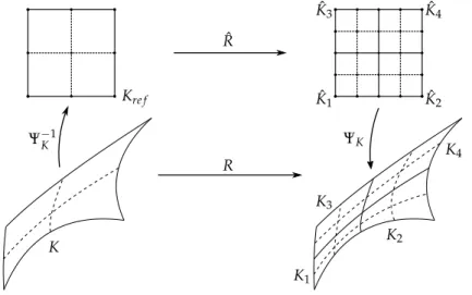
Figure 2 Example of second-order curvilinear element and mapping between reference and physical element. . . 29
Figure 3 Adaptive algorithm loop. . . 37
Figure 4 Characteristic size and characteristic lengths for a curvilinear element. . . 48
Figure 5 Example of computational grid with invalid distribution of refinement level and updated resolution after enforcing the 2 : 1 ratio. . . 50
Figure 6 Example of computational grid with invalid distribution of lo-cal polynomial degree and updated distribution after limiting the maximum jump in the local polynomial degree to one. . . 51
Figure 7 Dynamic adaptation algorithm. . . 51
Figure 8 Static adaptation algorithm. . . 52
Figure 9 Inviscid flow over a Gaussian bump at M = 0.5: Evolution of global entropy error Eq. (92) under uniform and adaptive
refinement. . . 61
Figure 10 Inviscid flow over a Gaussian bump at M = 0.5: Map of local polynomial degrees obtained based on different refinement indicators. . . 62
Figure 11 Laminar flow past a Joukowski airfoil at Re = 1000, M = 0.5, and α = 0◦: Convergence history of the drag coefficient under uniform and adaptive p-refinement. . . 64
Figure 12 Laminar flow past a Joukowski airfoil at Re = 1000, M = 0.5, and α = 0◦: L2-norm of the error in momentum density under uniform and adaptive p-refinement. . . 64
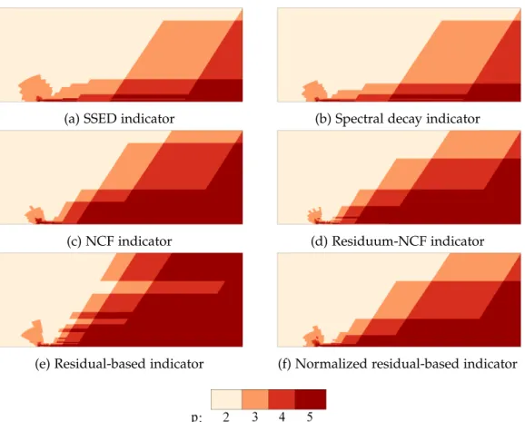
Figure 13 Laminar flow past a Joukowski airfoil at Re = 1000, M = 0.5, and α = 0◦: Local polynomial degree distribution obtained for different refinement indicators. . . 65
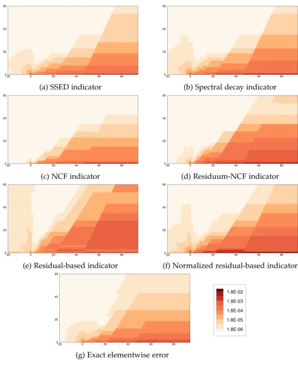
Figure 14 Laminar flow past a Joukowski airfoil at Re = 1000, M = 0.5, and α = 0◦: Close up view of local polynomial degree distribu-tion obtained for different refinement indicators. . . 66
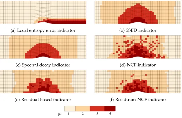
Figure 15 Laminar flow past a Joukowski airfoil at Re = 1000, M = 0.5, and α = 0◦: Refinement indicators (a) to (f) and error (g) for uniform polynomial degree p=2. . . 68
List of Figures xvii
Figure 16 Laminar flow past a Joukowski airfoil at Re = 1000, M = 0.5, and α = 0◦: Steps 3 to 5 of the refinement process using the NCF refinement indicator, NCF error distribution (top) and polynomial degree distribution (bottom). . . 69
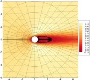
Figure 17 Laminar flow past a cylinder at Re = 40 and M = 0.1: Stream-lines and contour plot of the streamwise velocity. . . 70
Figure 18 Laminar flow past a cylinder at Re = 40 and M = 0.1: Evolution of the drag coefficient and corresponding error under uniform and adaptive p-refinement. . . 71
Figure 19 Laminar flow past a cylinder at Re = 40 and M = 0.1: L2-norm
of the error in the momentum density under uniform and adaptive p-refinement. . . 72
Figure 20 Laminar flow past a cylinder at Re = 40 and M = 0.1: Local polynomial degree distribution obtained for different refine-ment indicators in the near-wake region. . . 73
Figure 21 Laminar flow past a cylinder at Re = 40 and M = 0.1: Local polynomial degree distribution obtained for different refine-ment indicators in the far-wake region. . . 74
Figure 22 Laminar flow past a cylinder at Re = 100 and M = 0.1: Stream-lines and contour plots of the streamwise velocity of the av-erage flow field (left) and one realization of the instantaneous flow field (right). . . 75
Figure 23 Laminar flow past a cylinder at Re = 100 and M = 0.1: Convergence history of the time-averaged drag coefficient, the Strouhal number and the root mean square of the lift coefficient. 78
Figure 24 Laminar flow past a cylinder at Re = 100 and M = 0.1: Conver-gence history of root mean square of the momentum density components at location [3D, 0D](top) and time-averaged mo-mentum density components at location[3D, 1D](bottom). . . 79
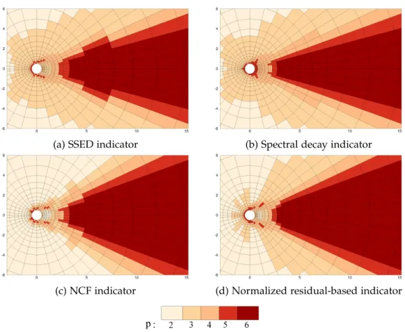
Figure 25 Laminar flow past a cylinder at Re = 100 and M = 0.1: Local polynomial degree distribution obtained for different refine-ment indicators. Near-wake region. . . 80
Figure 26 Laminar flow past a cylinder at Re = 100 and M = 0.1: Local polynomial degree distribution obtained for different refine-ment indicators. Far-wake region. . . 81
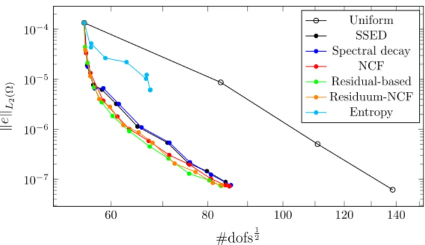
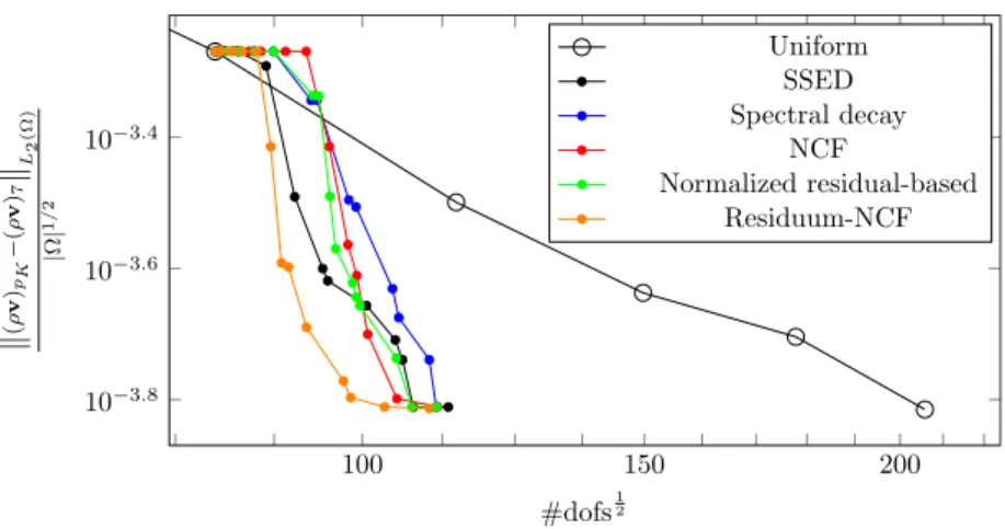
Figure 27 Inviscid flow over a Gaussian bump at M = 0.5: Global en-tropy error vs number of dofs and CPU time under uniform and adaptive refinement. . . 82
Figure 28 Schematic representation of h-refinement of a two-dimensional curvilinear element. . . 87
xviii List of Figures
Figure 29 Inviscid flow over a Gaussian bump at M = 0.5: Convergence history of the global entropy error under uniform and adaptive h-refinement. . . 88
Figure 30 Inviscid flow over a Gaussian bump at M = 0.5: Distribution of the local entropy error on the initial mesh. . . 89
Figure 31 Inviscid flow over a Gaussian bump at M = 0.5: Distribution of the local entropy error on the meshes obtained by adaptive h-refinement. The number of dofs is equal to ∼1202 for all refinement indicators with the exception of the local entropy error indicator, for which #dofs≈1002. . . . . 90
Figure 32 Inviscid flow over a Gaussian bump at M = 0.5: Adapted meshes and distribution of the local entropy error obtained by adaptive h-refinement. The number of dofs is equal to ∼1202
for all refinement indicators with the exception of the local entropy error indicator, for which #dofs≈1002. . . 91
Figure 33 Inviscid flow over a Gaussian bump at M = 0.5: Adapted meshes and distribution of the local entropy error obtained by adaptive h-refinement, close-up view. The number of dofs is equal to∼1202 for all refinement indicators with the exception
of the local entropy error indicator, for which #dofs≈1002. . . . 92
Figure 34 Laminar flow past a Joukowski airfoil at Re = 1000, M = 0.5 and α = 0◦: Convergence history of the drag coefficient under uniform and adaptive h-refinement. . . 93
Figure 35 Laminar flow past a cylinderat Re = 40 and M = 0.1: Con-vergence history of the drag coefficient under uniform and adaptive h-refinement. . . 94
Figure 36 Laminar flow past a Joukowski airfoil at Re = 1000, M = 0.5 and α = 0◦: Adapted meshes at the last iteration of adaptive h-refinement. Number of dofs are equal to ∼2802 and ∼2102 for the SSED and normalized residual-based indicator, respec-tively. Black lines: initial mesh. Blue lines: adapted mesh. . . . 95
Figure 37 Laminar flow past a cylinderat Re = 40 and M = 0.1: Adapted meshes at the last iteration of adaptive h-refinement. Number of dofs are equal to∼2502and∼1302for the SSED and normal-ized residual-based indicator, respectively. Black lines: initial mesh. Blue lines: adapted mesh. . . 96
List of Figures xix
Figure 38 Laminar flow past a Joukowski airfoil at Re = 1000, M = 0.5 and α = 0◦: Close-up view of adapted meshes near the leading edge (LE) and the trailing edge (TE) at the last iteration of adaptive h-refinement. Number of dofs are equal to∼2802and
∼2102 for the SSED and normalized residual-based indicator, respectively. Black lines: initial mesh. Blue lines: adapted mesh. 97
Figure 39 Example of computational grid (continuous black), equivalent graph (nodes and dashed lines) and a possible 2-way partition-ing. . . 101
Figure 40 Example of the evaluation of the volume and surface contri-butions to the vertex weights for an inviscid computation with the LLF flux on Intel Xeon Broadwell E5-2680v4 cores. Values are normalized by ωv(1, 2). . . 106
Figure 41 Example of the evaluation of the vertex weights, volume and total surface contribution for q = p+1 and an inviscid com-putation based on the LLF flux on Intel Xeon Broadwell E5-2680v4 cores. Values are normalized by ωv(1, 2). . . 107
Figure 42 Example evaluation of the vertex weights, volume and total surface contribution for q = p+1 and an LES using the Roe flux, BR2 scheme and Vreman model on Intel Xeon Broadwell E5-2690v4 cores. Values are normalized by ωv(1, 2). . . 108
Figure 43 Test configurations employed to analyse the graph partitioning algorithm. . . 110
Figure 44 Measured MPI imbalance for parallel computations for differ-ent definitions of the vertex weights in the graph partitioning algorithm. . . 111
Figure 45 Transport of a vortex by a uniform flow: Convergence history of the L2-norm of the error in the streamwise velocity
compo-nent u (left) and in the pressure (right) for uniform polynomial degree simulations and for dynamically p-adaptive simula-tions using various values of ηre f and ηcoars. In these tests,
∆tadapt =10∆t. . . 119
Figure 46 Transport of a vortex by a uniform flow: Distribution of the local polynomial degree (top half) and of the SSED indicator (bottom half) using the adaptive simulations for different val-ues of ηre f and ηcoars at t=10tc. In these tests,∆tadapt=10∆t. . 120
xx List of Figures
Figure 47 Transport of a vortex by a uniform flow: Convergence history of the L2-norm of the error in the streamwise velocity compo-nent (left) and in the pressure (right) for uniform polynomial degree simulations and for dynamically p-adaptive simula-tions using various values of ηre f and ∆tadapt. The coarsening
threshold is set here to ηcoars =10−2ηre f. . . 121
Figure 48 Transport of a vortex by a uniform flow: percentage of the total computational time of the simulation required by the error estimation procedure (left) and the resolution update step (right) as a function of ηre f for two values of ηcoars =
10−2ηre f (filled circles) and 10−3ηre f (empty circles), and three values of ∆tadapt: ∆t (black), 10∆t (red) and 100∆t (blue). . . 122
Figure 49 Dipole-wall collision at Re = 1000: Evolution of the total kinetic energy for uniform polynomial degree simulations (left) and dynamically p-adaptive simulations (right). . . 125
Figure 50 Dipole-wall collision at Re = 1000: Evolution of the total en-strophy for uniform polynomial degree simulations (left) and dynamically p-adaptive simulations (right). . . 126
Figure 51 Dipole-wall collision at Re = 1000: Error in the evolution of the total enstrophy (left) and total kinetic energy (right) as a function of the computational cost for uniform polynomial degree and dynamic p-adaptive simulations. . . 127
Figure 52 Dipole-wall collision at Re = 1000: Evolution of the total num-ber of dofs divided by the total numnum-ber of elements N for the dynamic p-adaptive simulations for different values of the refinement threshold ηre f. . . 127
Figure 53 Dipole-wall collision at Re = 1000: Contour plots of the vor-ticity field (top half) and distribution of the local polynomial degree (bottom half) at various instants of the dynamically p-adaptive simulation using ηre f =10−2. . . 129
Figure 54 Dipole-wall collision at Re = 1000: Percentage of the total computational time required for the error estimation and the update of the spatial resolution. . . 130
Figure 55 TGV at Re = 500: Evolution of the total kinetic energy (left) and of the total enstrophy (right) for the uniform polynomial degree and the adaptive simulations. . . 132
Figure 56 TGV at Re = 500: Close up view of the evolution of the total enstrophy. . . 132
Figure 57 TGV at Re = 500: Evolution of the total number of dofs for the dynamically p-adaptive simulations for two values of the refinement threshold. . . 133
List of Figures xxi
Figure 58 TGV at Re = 500: Isosurfaces of the Q-criterion (Q = 0.5) and slices of the local polynomial degree distribution for the dy-namically p-adaptive simulation with ηre f =10−3at times t = 7
and 12. . . 134
Figure 59 Laminar flow past a cylinder at Re = 100 and M = 0.1: Convergence history of the time-averaged drag coefficient, the Strouhal number and the root mean square of lift coefficient for the p-adaptive and uniformly p-refined simulations. . . 140
Figure 60 Laminar flow past a cylinder at Re = 100 and M = 0.1: Distri-bution of local polynomial degree obtained based on different refinement indicators, close-up view and streamlines. . . 141
Figure 61 Laminar flow past a cylinder at Re = 100 and M = 0.1: Distri-bution of local polynomial degree obtained based on different refinement indicators. . . 142
Figure 62 Laminar flow past a cylinder at Re = 100 and M = 0.1: Distribu-tion of local polynomial degree obtained based on the SSED-A indicator. Close-up view and streamlines of the average flow. . 143
Figure 63 DNS of the turbulent flow over periodic hills at Re = 2800: Geometrical configuration and employed mesh. . . 144
Figure 64 DNS of the turbulent flow over periodic hills at Re = 2800: Iso-surface of the Q-criterion (Q = 5) coloured by the streamwise velocity. . . 145
Figure 65 DNS of the turbulent flow over periodic hills at Re = 2800: Distribution of the refinement indicators computed from the baseline simulation with uniform polynomial degree p = 3. . . . 147
Figure 66 DNS of the turbulent flow over periodic hills at Re = 2800: Distribution of the three considered refinement indicators for three different values of the averaging time: from left to right Tavg = 2tc, 10tc and 18tc. . . 148
Figure 67 DNS of the turbulent flow over periodic hills at Re = 2800: Distribution of the local polynomial degree generated by the adaptive algorithm. . . 149
Figure 68 DNS of the turbulent flow over periodic hills at Re = 2800: Averaged velocity hui/ub at various locations obtained with
uniform polynomial degree and adaptive simulations com-pared to the reference DNS [32]. . . 152
Figure 69 DNS of the turbulent flow over periodic hills at Re = 2800: Averaged velocity hvi/ub at various locations obtained with
uniform polynomial degree and adaptive simulations com-pared to the reference DNS [32]. Values are shifted and scaled
xxii List of Figures
Figure 70 DNS of the turbulent flow over periodic hills at Re = 2800: Averaged velocity fluctuations hu0u0i/ub at various locations
obtained with uniform polynomial degree and adaptive simu-lations compared to the reference DNS [32]. Values are shifted
and scaled by a factor of 10. . . 154
Figure 71 DNS of the turbulent flow over periodic hills at Re = 2800: Averaged velocity fluctuations hu0v0i/ub at various locations
obtained with uniform polynomial degree and adaptive simu-lations compared to the reference DNS [32]. Values are shifted
and scaled by a factor of 30. . . 155
Figure 72 Transitional flow past a NACA0012 airfoil: Computational grid.158
Figure 73 Transitional flow past a NACA0012 airfoil: Distribution of the local polynomial degree generated by the adaptive algorithm. . 160
Figure 74 Transitional flow past a NACA0012 airfoil: Mesh resolution near the wall for the uniform polynomial degree simulation with p = 3 (blue) and for the adaptive simulations: V-SSED (green) and V-SSL (red). . . 161
Figure 75 Transitional flow past a NACA0012 airfoil: Isosurfaces of the Q-criterion (Q = 50) coloured by the streamwise velocity for the adaptive and the uniform polynomial degree simulations. 162
Figure 76 Transitional flow past a NACA0012 airfoil: Isosurfaces of the Q-criterion (Q = 50) and distribution of the local polynomial degree for the adaptive simulations. . . 162
Figure 77 Transitional flow past a NACA0012 airfoil: Skin friction coeffi-cient (left) and pressure coefficoeffi-cient (right) for the uniform and and for the adaptive simulations compared to the reference DNS data from Lehmkuhl et al. [119] and Zhang et al. [202]
(extracted). . . 163
Figure 78 Transitional flow past a NACA0012 airfoil: Pressure coefficient (left) and skin friction coefficient (right) for the adaptive sim-ulations with the SSL indicator using the WALE and Vreman model compared to the reference DNS data from Lehmkuhl et al. [119] and Zhang et al. [202] (extracted) . . . 165
Figure 79 Transitional flow past a NACA0012 airfoil: Averaged velocity profiles hui/U∞ and hvi/U∞ at various locations obtained with uniform polynomial degree and adaptive simulations compared to the reference DNS data from Lehmkuhl et al. [119]. . . 166
List of Figures xxiii
Figure 80 Transitional flow past a NACA0012 airfoil: Averaged velocity fluctuations profiles hu0u0i/U2∞ and hu0v0i/U∞2 at various lo-cations obtained with uniform polynomial degree and adap-tive simulations compared to the reference DNS data from Lehmkuhl et al. [119]. . . 167
Figure 81 Transitional flow past a NACA0012 airfoil: Averaged veloc-ity profileshui/U∞ andhvi/U∞ at various locations obtained with the adaptive simulations using the WALE and Vreman model, compared to the reference DNS data from Lehmkuhl et al. [119]. . . 168
Figure 82 Transitional flow past a NACA0012 airfoil: Averaged velocity fluctuations profileshu0u0i/U∞2 andhu0v0i/U∞2 at various loca-tions obtained with the adaptive simulaloca-tions using the WALE and Vreman model, compared to the reference DNS data from Lehmkuhl et al. [119]. . . 169
Figure 83 TGV at Re = 5 000: Energy spectra from the DNS computation (black) and the ideal DG-LES solution (blue) for various dis-cretizations: p = 7 and 723, 1443 and 2883 dofs. Dashed lines indicate the corresponding value of kDG(black) and ˜kDG(blue). 185
Figure 84 TGV at Re = 5 000: Ideal SGS dissipation spectrum for three discretizations with p = 7. The values ˜kDG and ˜kDG/2 are
marked by dash-dotted lines. . . 185
Figure 85 Energy spectra and relevant values of ˜kDG for the TGV at
Re = 20 000 (left), 40 000 (right). . . 186
Figure 86 TGV at Re = 20 000: Ideal SGS dissipation spectrum for three discretizations with p = 7. The values ˜kDG and ˜kDG/2 are
marked by dash-dotted lines. . . 187
Figure 87 TGV at Re = 40 000: Ideal SGS dissipation spectrum for three discretizations with p = 7. The values ˜kDG and ˜kDG/2 are
marked by dash-dotted lines. . . 187
Figure 88 Modal energy transfer for the ideal SGS stress for the TGV at Re = 5 000 (left), 20 000 (center), and 40 000 (right) for various discretizations with p=7. . . 188
Figure 89 TGV at Re = 20 000: Modal energy transfer for the ideal SGS stress for several discretizations with p=7. . . 189
Figure 90 Ideal modal eddy viscosity for the ideal subgrid stress for the TGV at Re = 5 000 (left), 20 000 (center), 40 000 (right) for various discretizations with p=7. . . 189
Figure 91 TGV at Re = 20 000: Ideal modal eddy viscosity for the ideal SGS stress using the BR1 and BR2 schemes. . . 190
xxiv List of Figures
Figure 92 TGV at Re = 20 000: Ideal modal energy transfer for the ideal SGS stress at various times for p =7 and 2883dofs. . . 191
Figure 93 TGV at Re = 20 000: Energy spectra of the DNS data and the ideal DG-LES solution for various discretizations for 1443, 2883
and 5763 dofs. Close-up view at frequencies between ˜kDG and
kDG. . . 192
Figure 94 TGV at Re = 20 000: Ideal SGS dissipation spectrum for various discretizations for 1443, 2883and 5763dofs. Dashed lines mark values of ˜kDGand ˜kDG/2. . . 192
Figure 95 TGV at Re = 20 000: Ideal modal energy transfer for various discretizations for 1443, 2883and 5763dofs. Dashed lines indi-cate mode-numbers m+1=0.75(p+1)and m= p. . . 193
Figure 96 TGV at Re = 20 000: Ideal modal eddy viscosity for various dis-cretizations for 1443, 2883and 5763dofs. Dashed lines indicate mode-numbers m+1=0.75(p+1)and m = p. . . 193
Figure 97 TGV at Re = 20 000: Ideal SGS dissipation spectrum for various discretizations for 1443, 2883and 5763dofs. Dashed lines mark values of ˜kDGand ˜kDG/2. . . 194
Figure 98 TGV at Re = 20 000: Ideal modal eddy viscosity for various dis-cretizations for 1443, 2883and 5763dofs. Dashed lines indicate mode-numbers m+1=0.75(p+1)and m = p. . . 195
Figure 99 TGV at Re = 20 000: Energy spectra of the DNS data, the ideal DG-LES solution, and DG-projection for three resolutions with p =7. Close-up view for frequencies between ˜kDGand kDG. . . 195
Figure 100 TGV at Re = 20 000: Ideal SGS dissipation spectrum of the ideal DG-LES solution and the DG-projection for three dis-cretizations with p = 7. Dashed lines mark values of ˜kDG and
˜kDG/2. . . 196
Figure 101 TGV at Re = 20 000: Ideal modal energy transfer of the ideal DG-LES solution and the DG-projection for three discretiza-tions with p = 7. Dashed lines indicate mode-numbers m+
1=0.75(p+1)and m = p. . . 196
Figure 102 TGV at Re = 20 000: Ideal modal eddy viscosity of the ideal DG-LES solution and the DG-projection for three dirscretiza-tions with p = 7. Dashed lines indicate mode-numbers m+
1=0.75(p+1)and m = p. . . 197
Figure 103 TGV at Re = 20 000, p=7, kDG =288: Ideal SGS energy transfer
(black solid), SGS model dissipation spectrum provided by the Smagorinsky model (dashed) and three variants of the DG-VMS approach for: β = 0.25 (green), β = 0.5 (blue), and β=0.75 (red) using the BR1 scheme. . . 198
List of Figures xxv
Figure 104 TGV at Re = 20 000, p=7, kDG=288: Ideal SGS energy transfer
(black solid), SGS model dissipation spectrum provided by the Smagorinsky model (dashed) and three variants of the DG-VMS approach for: β = 0.25 (green), β = 0.5 (blue), and β=0.75 (red) using the BR2 scheme (ηbr2=2). . . 200
Figure 105 TGV at Re = 20 000, p = 7, kDG = 288 : Ideal modal energy
transfer (black solid) and modelled modal energy transfer pro-vided by the Smagorinsky model (dashed) and three variants of the DG-VMS approach for: β=0.25 (green), β =0.5 (blue), and β=0.75 (red) using the BR1 scheme. . . 201
Figure 106 TGV at Re = 20 000, p = 7, kDG = 288 : Ideal modal eddy
viscosity (black solid) and modelled modal eddy viscosity pro-vided by the Smagorinsky model (dashed) and three variants of the DG-VMS approach for: β=0.25 (green), β =0.5 (blue), and β=0.75 (red) using the BR1 scheme. . . 201
Figure 107 TGV at Re = 20 000, p = 7, kDG = 288 : Ideal modal energy
transfer (black solid) and modelled modal energy transfer pro-vided by the Smagorinsky model (dashed) and three variants of the DG-VMS approach for: β=0.25 (green), β =0.5 (blue), and β=0.75 (red) using the BR2 scheme (ηbr2=2). . . 202
Figure 108 TGV at Re = 20 000, p = 7, kDG = 288 : Ideal modal eddy
viscosity (black solid) and modelled modal eddy viscosity pro-vided by the Smagorinsky model (dashed) and three variants of the DG-VMS approach for: β=0.25 (green), β =0.5 (blue), and β=0.75 (red) using the BR2 scheme (ηbr2=2). . . 202
Figure 109 TGV Re = 20 000: ideal SGS dissipation spectrum and model dissipation spectrum using the all-all DG-VMS approach using the BR2 scheme with ηBR2 = 2 for kDG = 288 and p = 3 (left),
p=8 (center) and p=11(right). . . 203
Figure 110 TGV Re = 20 000, p=7, kDG=144: Ideal SGS dissipation
spec-trum and modelled dissipation specspec-trum for mixed Smagorin-sky and DG-VMS models. . . 204
Figure 111 Distribution of the local effective Jacobian order for the 4-th order mesh for the flow over a Gaussian bump employed in Sec.5.3. . . 218
Figure 112 Distribution of the local effective Jacobian order for the 4-th order mesh for the flow over periodic hills. . . 218
Figure 113 Distribution of the local effective Jacobian order for a 4-th order C-type mesh around a NACA0012 airfoil. . . 219
Figure 114 TGV at Re = 20 000, t = 14, kDG = 144: Energy spectrum for
xxvi List of Figures
Figure 115 TGV at Re = 20, 000, t=14: Contour plot ofeν†(m)at constant
mz = 0 for p = 7 and 1443, 2883 and 5763 dofs (left to right)
using the BR1 scheme. . . 226
Figure 116 TGV at Re = 20, 000, t=14: Contour plot ofeν†(m)at constant
mz = 0 for p = 11 and 1443, 2883 and 5763 dofs (left to right)
L I S T O F TA B L E S
Table 1 Numerical parameters for the p-adaptive algorithm. . . 60
Table 2 Integral flow quantities obtained through numerical simula-tions and experiments in the literature and for the present reference simulation for the flow past a cylinder at Re=100. . 77
Table 3 TGV at Re = 500: Computational cost of uniform polynomial degree and dynamically p-adaptive simulations. . . 133
Table 4 DNS of the turbulent flow over periodic hills at Re = 2800: Computational cost of simulations expressed in terms of num-ber of dofs and computational time required to simulate a time interval h/ubmeasured on 280 Intel Xeon Broadwell E5-2690v4
cores. Note: the uniform polynomial degree simulation with p = 3 presents a value of∆t that is 2.5 times that of all the other simulations. . . 150
Table 5 Summary of geometrical parameters for the computational do-main of selected studies of the flow past a NACA0012 airfoil at medium Reynolds numbers and low incidence. . . 157
Table 6 Transitional flow past a NACA0012 airfoil: Comparison be-tween current LES results and reference computations from the literature. From the left: Aerodynamic coefficients, sepa-ration and reattachment points, number of dofs, CPU time to advance the simulation for 105 time steps, and physical time step∆t. CPU time measured on 840 Intel Xeon Broadwell E5-2690v4 cores. . . 159
Table 7 TGV at Re = 20 000, p = 7, kDG = 288: Model coefficients
selected for the Smagorinsky and DG-VMS model using the BR1 and BR2 schemes. . . 198
A C R O N Y M S
CFD Computational Fluid Dynamics DG discontinuous Galerkin
DE Discretization error
DNS Direct Numerical Simulation dofs Degrees of freedom
FD Finite Difference FE Finite Element
FV Finite Volume
HiOCFD International Workshop on High-Order CFD Methods HPC High performance computing
ILES Implicit Large Eddy Simulation LSB Laminar separation bubble MGS Modified Gram-Schmidt MPI Message passing interface
NCF Non-conformity
NS Navier-Stokes
LES Large Eddy Simulation
RANS Reynolds Averaged Navier-Stokes RE Residual error
SGS Subgrid-scale
SIP Symmetric interior penalty SSED Small-scale energy density SSL Small-scale Lifted
SSP Strong Stability Preserving TE Truncation Error
TGV Taylor-Green Vortex VMS Variational Multiscale
C H A P T E R
1
I N T R O D U C T I O Nr é s u m é d u c h a p i t r e e n f r a n ç a i s
Ce chapitre est dédié à l’introduction et à la définition des objectifs de ce travail de recherche et à la description du document de thèse.
L’un des défis les plus importants pour l’application de la mécanique des fluides numérique (CFD) aux applications industrielles est le coût de calcul exigé par la sim-ulation des écoulements turbulents avec résolution d’échelles. Plusieurs approches sont brièvement décrites dans ce chapitre illustrant l’intérêt pour le développement des techniques de simulation des grandes échelles (LES).
Afin de promouvoir l’application des simulations LES sur des configurations avancées, de nouvelles méthodes numériques qui réduisent les erreurs de dissipation et de dispersion et permettent d’obtenir une efficacité parallèle élevée sur des architectures de mémoire distribuée sont nécessaires. Une méthode qui présente des propriétés intéressantes pour le développement d’approches LES est la méthode Galerkine discontinue (DG). Les principaux avantages de la méthode DG et les principaux défis ouverts sont ainsi décrits dans la Sec.1.1.
Le travail de thèse porte sur l’amélioration de la précision et de l’efficacité des méthodes DG-LES. Deux axes de recherche sont analysés à cette fin : le développe-ment de stratégies de résolution adaptatives et l’analyse de modèles LES pour les méthodes de DG de haut niveau. Celles-ci sont présentées dans la Sec.1.2.
Le cadre de recherche et les outils utilisés sont ensuite décrits dans la Sec.1.3. En
particulier, nous décrivons le solveur DG ainsi que la plate-forme de calcul à haute performance utilisés dans les travaux réalisés. De plus, les collaborations établies dans le cadre de cette étude sont présentées.
Enfin, les chapitres décrivant les travaux réalisés sont résumés dans la Sec.1.4.
1.1 i n t r o d u c t i o n
Computational Fluid Dynamics (CFD) is nowadays a fundamental tool for the predic-tion and analysis of flows in both industrial and academic applicapredic-tions.
2 i n t r o d u c t i o n
In the scientific community, CFD is employed for the analysis of the physical mechanisms governing the motion of fluids. The main objective is to improve the understanding of these mechanisms to be able to model and control them. In this context CFD must accurately reproduce complex phenomena on relatively simplified configurations.
In industry, particularly in the aerospace and automotive fields, CFD is used throughout the development cycle of products, starting from the preliminary design phases, to the optimization and the analysis of the performance of the final product. For this type of applications, CFD must thus provide reliable results on complex configurations and within short turn-around times.
Despite the rapid improvement of these techniques and the maturity of advanced simulation tools available, there are still several challenges that limit the range of applications of CFD. This implies that experimental results are still required to verify the accuracy of numerical predictions. One of these challenges is the prohibitive computational cost required for the accurate simulation of turbulent flows, which are characterized by a chaotic three-dimensional mixing behaviour and exhibit a wide range of spatial and temporal scales.
The accurate simulation of such flows without any modelling assumptions requires the resolution of all the turbulent scales. This approach is commonly referred to as Direct Numerical Simulation (DNS) and presents a prohibitive computational cost for most industrial applications, which are characterized by high Reynolds numbers and complex geometries. The most commonly employed approach to reduce this com-putational cost consists in modelling all the turbulent scales and only resolving the mean flow. This strategy is known as Reynolds-Averaged Navier-Stokes (RANS) and is nowadays the standard industrial approach. Several works have shown, however, that RANS type approaches present serious limitations. They often require the ad-hoc choice of the RANS model and the tuning of the model parameters. Furthermore, this approach is often unable to predict unsteady large-scale phenomena and separated flows. These phenomena are typically encountered in critical off-design conditions in many aeronautical applications.
An intermediate approach between DNS and RANS is called Large Eddy Simu-lation (LES) and consists in resolving the largest energy-containing turbulent scales and modelling only the smallest turbulent scales. This approach is justified by the universal character of the smallest scales of turbulence, which, in principle, allows for a reduction of the modelling assumptions and a more general description of the behaviour of these flows.
Despite the reduction of the computational cost of LES with respect to DNS and the large number of works demonstrating improved results compared to RANS ap-proaches, LES is seldom applied in the industrial context. This is due to the high com-putational cost for the accurate simulation of the largest three-dimensional unsteady turbulent scales. In order to promote the application of LES to industrial problems,
1.1 introduction 3
new numerical methods must be developed with low dispersion and dissipation errors and which can take full advantage of recent progress in high performance computing (HPC) to provide accurate results in reasonable times.
The Finite Volume (FV) method is currently the most employed numerical method for the simulation of flows in industrial applications. This is due to their robustness and relatively simple formulation for any polyhedral elements in structured and un-structured approaches and therefore their capability of handling complex geometries. Typical FV methods are however of first or second order, i. e. the error of the solution is proportional to the characteristic mesh size or to its square. In order to obtain sufficiently low dissipation and dispersion errors for LES, second-order methods require very fine meshes and therefore a prohibitively large number of degrees of freedom. Despite recent developments in higher-order FV methods, they still require the use of large stencils which can increase the computational cost and decrease their robustness in the case of stiff unstructured meshes and reduces the parallel efficiency of the algorithm.
For this reason, academic research focusing on the analysis of turbulent flows has made extensive use of alternative high-order methods such as high-order finite difference (FD), spectral and pseudo-spectral methods. These approaches allow for a large reduction of the dissipation and dispersion errors but rely on the use of structured meshes and are often limited to the analysis of simplified geometries.
Recent years have seen therefore a growing interest and rapid progress in the development of various methods which combine high-order accuracy with the flexi-bility of FV methods for the analysis of complex industrial configurations. Examples of these approaches are the discontinuous Galerkin (DG) method [46], the Spectral
Element method (SEM) [101], the Spectral Difference (SD) method [123], and the Flux
Reconstruction (FR) method [97].
Among these, the DG method, based on the variational formulation of the set of equations to be solved, combines features of FV and Finite Element (FE) methods and presents a number of advantages for LES of industrial applications. In the DG method, the solution is represented by a linear combination of polynomials within each element similarly to FE approaches. However, similarly to FV approaches, the solution is assumed to be discontinuous across element interfaces, requiring the definition of numerical fluxes.
By modifying the polynomial degree of the representation of the solution, the DG method can achieve arbitrary order of accuracy while employing unstructured and non-conforming meshes. In contrast to high-order FV methods, the order of accu-racy is also preserved near physical boundaries. Additionally, the spatial resolution can be efficiently adapted by modifying the local mesh size (h-adaptation) or the local polynomial degree of the representation of the solution within each element (p-adaptation). These properties allow for the analysis of complex geometrical con-figurations typical of industrial applications.
4 i n t r o d u c t i o n
High-order DG methods are also particularly suited for modern HPC architectures, achieving high parallel efficiency on distributed memory machines. This is due to the compact stencil of the scheme, as the evaluation of numerical fluxes only requires the knowledge of the solution inside the element and at the interface with its direct neighbours.
Finally, if hierarchical bases are employed, the variational formulation on which these methods rely allows for the natural application of multilevel LES models such as the Variational Multiscale approach, which has shown promising results in a number of applications [50].
There are, however, still a number of challenges that hinder the application of high-order DG methods to industrial applications. One of these limitations is the reduction of the local order of accuracy in the presence of geometrical or physical discontinuities, such as shock waves. These introduce numerical oscillations and require shock-capturing techniques in order to obtain stable solutions [151].
It is also important to take into account the lack of significant experience for the generation of curvilinear meshes for industrial applications using high-order methods. This is due to the limited number of advanced high-order mesh generators available and the relatively recent application of high-order methods to industrial problems [196].
The development of adaptive spatial resolution techniques represents a solution to these challenges and can considerably reduce the computational cost of simula-tions. On the one hand, by measuring the local regularity of the solution, adaptive resolution strategies can reduce the local mesh size in the presence of discontinuities, thereby isolating them and reducing the generation of numerical oscillations and er-rors. Similarly, the local order of the method can be increased in regions characterized by smooth solutions, thus efficiently improving the accuracy of simulations. On the other hand, adaptive resolution strategies reduce the amount of expertise required by the user, as error estimation techniques are used to measure the local quality of the solution and identify the local resolution requirements. The development of error estimation and resolution adaptive strategies is thus particularly relevant in the framework of LES. This is due to the high computational cost of simulations and the difficulties in assessing their quality.
Another relevant research subject is the development of accurate LES models in the context of high-order schemes. In the framework of DG methods two main strategies are employed for performing LES. One possible approach, referred to as implicit LES (ILES), consists in taking advantage of the dissipation properties of the numerical scheme or specific stabilization techniques in order to mimic the dissipative effect of the unresolved scales, see e. g. [74, 142, 188]. A second strategy consists in the
discretization of LES models developed in the continuous framework without taking into account the effect of the numerical discretization [205].
1.2 objective of the thesis 5
Only a limited number of works have recently started to develop LES models specifically tailored for high-order FE-type methods, e. g. [41, 42]. The analysis of
the influence of the parameters of the hp-discretization, such as the local polynomial degree and the discretization of the numerical fluxes, on these models represents therefore an important research topic to promote the use of DG-LES approaches.
1.2 o b j e c t i v e o f t h e t h e s i s
The main objective of the present work is to improve the accuracy and the compu-tational efficiency of DG-LES methods. To this end, two main lines of research are analysed: the development of adaptive resolution strategies and the analysis of LES models in the context of high-order DG methods.
As regards the first topic, resolution adaptation strategies analyse the local solution quality and the resolution requirements. They allow for the optimization of the spatial discretization to improve the accuracy of simulations for a fixed computational cost or reduce the computational cost for a fixed level of accuracy. One of the most important factors determining the efficiency of a resolution adaptation algorithm is the choice of the error estimation strategy. The first part of this thesis is therefore dedicated to the analysis of various error estimation strategies derived from the literature. Discretization-error and residual-error based indicators are compared for the purpose of identifying advantages and drawbacks of these indicators for the development of both p- and h-adaptation strategies.
In the case of large scale computations, high parallel efficiency on distributed memory architectures must be preserved for the adaptive computations to reduce the total computational time. This requires the development of load balancing techniques which can take into account the computational load dependency on the local polyno-mial degree (for p-adaptation) and on the number of interfaces (for h-adaptation) of each element in the computational grid.
In the second part of this work, we then study p-adaptation strategies for the simulation of unsteady flows and, in particular, for LES of turbulent flows. The focus on p-adaptation is due to the potentially higher efficiency of this technique, as regards the reduction of dissipation and dispersion errors, for scale-resolving simulations of turbulent flows at relatively low Mach numbers.
Both static and dynamic p-adaptation strategies are studied. Static adaptation allows for the reduction of the computational cost of the LES of statistically steady flows, for which the resolution requirements remain approximately unchanged over time. Dynamic adaptation, on the other hand, presents higher complexity but can provide a further reduction of the computational cost for unsteady problems, in par-ticular for transient flows presenting significant variation over time of the resolution requirements.
6 i n t r o d u c t i o n
The computational gain provided by the algorithms developed in this thesis is analysed through several numerical experiments. We measure, in particular, the re-duction of the number of degrees of freedom and of the computational time required to achieve a target level of accuracy.
The second research topic considered in this work is the analysis of LES models for high-order DG methods. For this purpose, a novel framework is developed for the a-priori analysis of DG-LES models taking into account the effect of the numerical discretization. This analysis aims at improving the current understanding of the influence of the hp-discretization on the resolution properties of the scheme in the con-text of scale-resolving simulations and in defining the separation between resolved and unresolved scales. The proposed methodology is applied for the analysis of the Variational Multiscale approach [93], which has been shown to provide improved
predictions of turbulent flows as compared to classical LES models. Various open questions, however, hinder its systematic application for configurations of industrial interest. The developed framework is therefore used to study the accuracy of the VMS approach in combination with the DG discretization and suggest guidelines for the selection of the model parameters.
1.3 c o n t e x t o f t h e t h e s i s
This research is carried out in the framework of the development of the high-order DG solver Aghora at ONERA. The Aghora solver is implemented in Fortran90 and uses the message passing interface (MPI) to perform parallel computations on distributed memory machines. Based on both the modal and the nodal DG formulations on unstructured meshes, it is designed for the simulation of compressible flows with a variety of mathematical, numerical, and physical models. The verification of the solver and the analysis of its accuracy and performance has already been the subject of several publications [42,43,125,205] and collaborations, namely in the framework
of European projects [110,162].
The computations carried out in this research project have been performed on two supercomputing platforms: Sator and Occigen.
Sator is a supercomputer produced by NEC corporation and has been acquired by ONERA in 2017. At the time of writing, it is composed of two types of nodes. A first group comprises 620 nodes each equipped with two Intel Xeon «Broadwell» E5-2680v4 processors with 14 cores at 2.4 GHz and 35 MB cache and a total of 128 GB of RAM. A second group of 160 nodes is composed of two Intel Xeon «Skylake-6152» processors with 22 cores at 2.1 GHz and 30.25 MB cache and presents 192 GB of RAM. Inter-node connection is based on the low latency Intel Omnipath Architecture fabrics running at 100 Gbps.
Thanks to two grants offered by GENCI (Grand Equipement National de Calcul In-tensif) under projects A0022A10129 and A0032A10309, some of the computations
pre-1.4 outline of the thesis 7
sented in this thesis have been performed on the HPC platform called Occigen, owned by GENCI and operated by CINES (Centre Informatique National de l’Enseignement Superieur). Produced by Atos-Bull, it is currently ranked as the 70th supercomputer in the Top500 world ranking of June 2018. Occigen is equipped with 2016 nodes each composed of two Intel Xeon «Haswell» E5-2690v3 processors with 12 cores at 2.6 GHz, and 1260 nodes composed of two Intel Xeon «Broadwell» E5-2690v4 processors with 14 cores at 2.6 GHz. Each node is equipped with 128 GB (Haswell) or 64 GB of RAM (Broadwell) and inter-node communication is provided by Intel Infiniband fabrics running at 56 Gbps.
This PhD thesis has been fully supported by the Marie Skłodowska-Curie Inno-vative Training Network (ITN) Stability and Sensitivity Methods for Industrial Design (SSeMID) [168] funded by the European Union’s Horizon 2020 research and
innova-tion programme. As such, over the course of the project, several collaborainnova-tions have been established within the framework of this ITN. These include two joint research projects with J. Marcon and the research group of Pr. J. Peiro and Pr. S. Sherwin at Imperial College London, and with A. Rueda Ramirez, in the research group of Pr. E. Valero, at the Universidad Politécnica de Madrid.
Finally, part of the research work presented in Chap. 10 has been carried out
in the framework of the 2018 Summer Program at the Center for Turbulence Re-search, at Stanford University. This study has been part of a collaboration with Pr. E. Lamballais from the Université de Poitiers, Pr. M. Massot from École Polytech-nique, and K. Bando and the research group of Pr. M. Ihme from Stanford University.
1.4 o u t l i n e o f t h e t h e s i s
This dissertation is organized as follows.
In Chap.2we present an overview of the physical models employed throughout
this work. After a brief description of the Navier-Stokes equations govern-ing the motion of compressible flows, we discuss the different approaches for scale-resolving simulations to justify the interest in the development of LES techniques. Two different approaches for deriving the LES equations are then introduced, the classical approach based on spatial filters and the variational approach based on the projection on a discrete solution space.
Chap.3focuses on the description of the DG numerical discretization employed
throughout the present work. Following a brief presentation of the history of the development of DG methods, the relevant formulation of the spatial and temporal discretization of these methods is introduced.
Chap. 4 presents an overview of resolution adaptation strategies. Adaptation
techniques based on h- and p-adaptation are described highlighting the advan-tages and drawbacks of the different approaches. The resolution adaptation
8 i n t r o d u c t i o n
algorithm for steady problems is then described and various error estimation and marking strategies are outlined. In particular, in Sec. 4.4.6 we present a
novel error estimation strategy developed over the course of this work. Different strategies for the application of adaptive approaches to unsteady problems are then discussed. Finally, the difficulties associated with the development of refinement indicators for LES are presented.
Chap. 5 provides a comparison of different refinement indicators for the
de-velopment of p-adaptive simulations. The efficiency of different refinement indicators is initially analysed by performing numerical simulations of inviscid and viscous steady flows. The convergence history of a number of relevant quantities of interest and the distribution of the local polynomial degree ob-tained from the use of the considered indicators are studied. The applicability of the results obtained to unsteady flow simulations is then demonstrated. Finally, a comparison of the computational cost and potential implementation issues associated with the different refinement indicators is presented.
In Chap. 6 we analyse the suitability of the considered error estimation
strate-gies for the development of an h-adaptive algorithm based on element splitting. For this purpose, the comparison presented in Chap.5is extended by
perform-ing h-adaptive simulations.
In Chap. 7 we discuss the development of a load balancing algorithm for
h- and p-adaptive simulations. At first, the graph partitioning algorithm is briefly described highlighting the requirement to obtain accurate estimates of the non-uniform distribution of the computational load for h/p-adaptive simulations. An approach to calibrate the load balancing algorithm from direct performance measurements is then introduced. The effectiveness of the developed strategy in providing well-balanced partitionings is demonstrated by performing numerical experiments on configurations using non-uniform polynomial degree.
Chap.8discusses the development of a dynamic p-adaptation algorithm. After
a brief description of the proposed algorithm, dynamically p-adaptive simula-tions of three different configurasimula-tions are performed: the transport of a vortex by a uniform inviscid flow, the collision of a dipole with a no-slip boundary, and the Taylor-Green Vortex at Re = 500. The considered configurations allow for the analysis of the performance of the dynamic algorithm and of the influ-ence of various parameters on the accuracy and the computational cost of the simulations.
In Chap.9 we present a static p-adaptation algorithm for scale-resolving
simu-lations. At first, different strategies to define refinement indicators for the static adaptation of unsteady problems are presented. These are initially compared by performing statically p-adaptive simulations of the periodic laminar flow
1.4 outline of the thesis 9
past a cylinder. The applicability of the results obtained to the static adaptation of statistically steady turbulent flows is analysed by studying the flow over periodic hills. Finally, adaptive LES of the transitional flow past a NACA0012 airfoil are performed. It is shown that the novel error estimation strategy developed in this work can be employed to efficiently improve the accuracy of LES.
Chap.10discusses the a-priori analysis of DG-LES models. We propose a novel
framework to carry out energy transfer analyses of DG-LES models from DNS databases. A-priori analyses of the DG-VMS approach are then presented. Its accuracy in reproducing the ideal energy transfer mechanism between resolved and unresolved scales is analysed. The influence of various formulations and model parameters are discussed and guidelines for further developments are presented.
Chap. 11 presents the main conclusions of this research, alongside possible
C H A P T E R
2
T H E P H Y S I C A L M O D E Lr é s u m é d u c h a p i t r e e n f r a n ç a i s
Ce chapitre est dédié à la description des équations de modélisation physique utilisées dans cette étude.
Après avoir brièvement présenté les équations de Navier-Stokes (NS), qui régissent le mouvement d’un fluide compressible, dans la Sec. 2.3 nous nous concentrons
sur la description des différentes approches de modélisation physique qui peuvent être utilisées pour la simulation des écoulements turbulents. Celles-ci vont de la simulation numérique directe (DNS), qui résout toutes les échelles turbulentes, à l’approche Reynolds Averaged Navier-Stokes (RANS), qui décrit l’évolution de la moyenne d’ensemble des écoulements en modélisant toutes les échelles turbulentes. Dans ce contexte, la simulation des grandes échelles (LES pour Large Eddy Simu-lation) représente une approche intermédiaire. Dans cette approche, une fraction limitée des échelles turbulentes est résolue, correspondant aux grandes échelles, alors que l’effet des échelles non résolues sur les échelles résolues est modélisé.
Le reste de ce chapitre est dédié à la formulation des équations LES et à la présenta-tion des modèles de sous-mailles LES utilisés dans cette étude. Deux approches pour la dérivation des équations du LES sont présentées. La première approche, classique, est décrite dans la Sec. 2.4. Elle consiste à dériver les équations LES en filtrant les
équations NS à l’aide d’un filtre de convolution. Le deuxième approche consiste à projeter les équations NS sur un espace fonctionnel associé à la discrétisation spatiale. Cette approche, fondée sur une formulation variationnelle des équations LES, est présentée dans la Sec. 2.5.
La formulation variationnelle des équations LES est employée dans la Sec.2.6pour
introduire l’approche Variational Multiscale (VMS). Elle consiste à séparer les échelles résolues en deux composantes: une composante à grande échelle, supposée sans interaction avec les échelles non résolues, et une composante à petite échelle. En limitant l’effet du modèle de sous-maille aux petites échelles résolues, il a été dé-montré que l’approche VMS améliore la prédiction des simulations LES en réduisant l’excès de dissipation introduit par les modèles LES standard mono-échelle sur les plus grandes échelles résolues.