CASE STUDY
Bactrocera
dorsalis
OF THE SPECIFIC
PHYTOSANITARY
SURVEILLANCE SYSTEM
DEWEY 632.77 AGRIS
H10
Guidelines for the implementation of the Specific Phytosanitary Surveillance System: case study: Bactrocera Dorsalis by IICA is
published under license Creative Commons Attribution-ShareAlike 3.0 IGO (CC-BY-SA 3.0 IGO) (http://creativecommons.org/licenses/by-sa/3.0/igo/)
Based on a work at www.iica.int
IICA encourages the fair use of this document. Proper citation is requested.
This publication is available in electronic (PDF) format from the Institute's Web site: http://www.iica.int
Editorial coordination: Lourdes Fonalleras and Florencia Sanz Translator: Paula Fredes
Layout: Victor Hugo Vidart Cover design: Victor Hugo Vidart Digital printing
Guidelines for the implementation of the Specific Phytosanitary Surveillance System: case study: Bactrocera Dorsalis / Inter-American Institute for Cooperation on Agriculture, Comité Regional de Sanidad Vegetal del Cono Sur; José Manuel Galarza. – Uruguay : IICA, 2018. A4; 21 cm x 29,7 cm.
ISBN: 978-92-9248-785-0 Published also in Spanish
1. Pests of plants 2. Bactrocera dorsalis 3. Crops 4. Citrus 5. Hosts 6. Pest monitoring 7. Risk management 8. Environmental factors 9. Cartography I. IICA II. COSAVE III. Title.
Pablo Cortese, Ignacio García Varona, Federico Aguirre, Oscar Von Baczko, Yanina Outi from Servicio Nacional de Sanidad y Calidad Agroalimentaria – SENASA from Argentina;
Luis Sánchez Shimura, Remi Castro Ávila, Gustavo López Zenteno, Edgar Delgado Vargas, Immer Adhemar Mayta Llanos, Geordana Zeballos from Servicio Nacional de Sanidad Agropecuaria e Inocuidad Alimentaria – SENASAG from Bolivia; Ricardo Kobal Raski, Dalci de Jesus Bagolin, Jesulindo de Souza Junior, Ériko Tadashi Sedoguchi from Secretaria de Defensa Agropecuaria del MAPA from Brasil;
Marco Muñoz, Fernando Torres Parada, Jairo Eladio Alegría Contreras, Carolina Pizarro, Karina Reyes, Ilania Astorga from Servicio Agrícola y Ganadero – SAG from Chile;
The Guide for the Implementation of Specific Phytosanitary Surveillance System has been applied through two case studies. Those products were
developed as a result of the component aimed at strengthening plant pest surveillance in the framework of STDF / PG / 502 Project "COSAVE: Regional Strengthening of the Implementation of Phytosanitary Measures and Market Access". The beneficiaries are COSAVE and the NPPOs of the seven countries that make up COSAVE. The Standards and Trade
Development Facility (STDF) fund it, the Inter-American Institute for Cooperation on Agriculture (IICA) is the implementing organization and the IPPC Secretariat supports the project.
The editorial coordination was in charge of Maria de Lourdes Fonalleras and Florencia Sanz.
Maria de Lourdes Fonalleras, Florencia Sanz y José Manuel Galarza, have defined the original structure of this Guide.
The content development corresponds exclusively to José Manuel Galarza expert contracted especially for the project.
The technical readers that made important contributions to develop the study cases are the specialists of the NNPO's participating in the Project:
Aquino, Liz Adriana Ojeda, Rosa Liliana Encina, María Bettina Chaparro from Servicio Nacional de Calidad, Sanidad Vegetal y de Semillas – SENAVE from Paraguay; Moisés Pacheco Enciso, Johny Naccha Oyola, Cecilia Lévano Stella, Betty Matos Nonogawa, Carmen Oré Vento, Iván Gutiérrez Martínez, Jorge Velapatiño Flores, Percy Alberto Mamani Sánchez from Servicio Nacional de Sanidad Agraria – SENASA from Perú;
Elina Zefferino and Noelia Casco from Dirección General de Servicios Agrícolas – DGSA/ MGAP from Uruguay.
We express special appreciation to all of them. We also thank the support received from the IPPC
Secretariat for the implementation of this component of the project.
Finally, we thanks Víctor Vidart by diagramming the document.
1.
PURPOSE
Detection surveillance of Bactrocera dorsalis (Hendel) in citrus crops in the COSAVE region.
2.
SCOPE
COSAVE region, considering pest entry routes, citrus host distribution and suitable environmental conditions for the pest.
3.
TARGET PEST
Bactrocera dorsalis (Hendel), see the pest datasheet in Annex 1.
4.
DURATION AND APPROPRIATE TIMING
The duration is one (1) year, particularly in the seasons with more trade and passenger flows, with a biweekly frequency between assessments. It is important to consider host phenology for the identification of the right time for the surveys.
5.
SITE SELECTION
For the area or site selection process, the following information is required in advance:
• Cadastral map of the region
• Hydrography and geographical characteristics (forests, mountains, lakes, rivers, deserts) in the location
• Risk map for the region
• Area and production of hosts at the political and administrative level as detailed as possible
• Location of risk ports and airports • International transport routes
5.1. Environmental modeling for the development of risk maps for the region The environmental niche modeling is commonly used to develop probabilistic maps of species distribution. Among the available modeling techniques, MaxEnt has become one of the most popular tools for modeling species distribution, with hundreds of peer-reviewed articles published each year. The popularity of MaxEnt is mainly due to the short running time, easy operation, small sample size, high simulation precision, the use of a graphical interface and automatic parameter configuration capacities (Morales et. al, 2017; Costa P., Holtz V. 2011; Wang R. et al. 2018).
Risk maps for the target pest can be managed for the risk characterization and the regional prioritization of surveillance activities. In this study case, we use the MaxEnt model to identify the environmental risk for Bactrocera dorsalis with worldwide locations that report the pest and their correlation with the bioclimatic variables from the Worldclim database (http://www.worldclim.org/).
The details of the method appear in Annex 2, and the resulting regional environmental risk map appears in Figure 1. The areas in red and yellow color mean higher and medium risk respectively, the light blue color means lower estimated risk. The risk estimation is based on MaxEnt results and the
comparison of the presence of the pest and the bioclimatic variables where the pest is reported.
Fig. 1. Environmental risk map of Bactrocera dorsalis for the COSAVE region. Higher risk in red, medium risk in yellow and lower risk in light blue. Scale 1:45,000,000. Source: Prepared for STDF/PG/502 COSAVE Project.
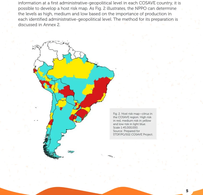
Fig. 2. Host risk map—citrus in the COSAVE region. High risk in red, medium risk in yellow and low risk in light blue. Scale 1:45,000,000. Source: Prepared for
STDF/PG/502 COSAVE Project.
5.2. Host area in the region
Bactrocera dorsalis is a very polyphagous pest with many hosts mentioned in its
datasheet (Annex 1). In order to explain the details of the surveillance, citrus is selected as the target host. citrus production is growing in all countries of the region and is a highly important activity. It accounts for about 134,034 hectares in Argentina, 51,211 in Bolivia, 766,085,227 in Brazil, 19,324 in Chile, 51,786 in Peru, 18,324 in Paraguay, and 15,394 hectares in Uruguay. Based on citrus production information at a first administrative-geopolitical level in each COSAVE country, it is possible to develop a host risk map. As Fig. 2 illustrates, the NPPO can determine the levels as high, medium and low based on the importance of production in each identified administrative-geopolitical level. The method for its preparation is discussed in Annex 2.
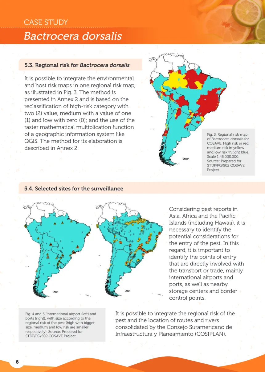
5.4. Selected sites for the surveillance
Fig. 4 and 5. International airport (left) and ports (right), with size according to the regional risk of the pest (high with bigger size, medium and low risk are smaller
Fig. 3. Regional risk map of Bactrocera dorsalis for COSAVE. High risk in red, medium risk in yellow and low risk in light blue. Scale 1:45,000,000. Source: Prepared for STDF/PG/502 COSAVE Project.
5.3. Regional risk for Bactrocera dorsalis It is possible to integrate the environmental and host risk maps in one regional risk map, as illustrated in Fig. 3. The method is
presented in Annex 2 and is based on the reclassification of high-risk category with two (2) value, medium with a value of one (1) and low with zero (0); and the use of the raster mathematical multiplication function of a geographic information system like QGIS. The method for its elaboration is described in Annex 2.
It is possible to integrate the regional risk of the pest and the location of routes and rivers
consolidated by the Consejo Suramericano de Considering pest reports in Asia, Africa and the Pacific Islands (including Hawaii), it is necessary to identify the potential considerations for the entry of the pest. In this regard, it is important to identify the points of entry that are directly involved with the transport or trade, mainly international airports and ports, as well as nearby storage centers and border control points.
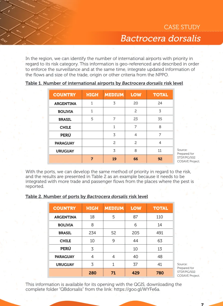
ARGENTINA 1 3 20 24 BOLIVIA 1 2 3 BRASIL 5 7 23 35 CHILE 1 7 8 PERÚ 3 4 7 PARAGUAY 2 2 4 URUGUAY 3 8 11 7 19 66 92
COUNTRY HIGH MEDIUM LOW TOTAL
In the region, we can identify the number of international airports with priority in regard to its risk category. This information is geo-referenced and described in order to enforce the surveillance and at the same time, integrate updated information of the flows and size of the trade, origin or other criteria from the NPPO.
Table 1. Number of international airports by Bactrocera dorsalis risk level
With the ports, we can develop the same method of priority in regard to the risk, and the results are presented in Table 2 as an example because it needs to be integrated with more trade and passenger flows from the places where the pest is reported.
Table 2. Number of ports by Bactrocera dorsalis risk level
ARGENTINA BOLIVIA BRASIL CHILE PERÚ PARAGUAY URUGUAY
COUNTRY HIGH MEDIUM LOW TOTAL
18 5 87 110 8 6 14 234 52 205 491 10 9 44 63 3 10 13 4 4 40 48 3 1 37 41 280 71 429 780
This information is available for its opening with the QGIS, downloading the complete folder “QBdorsalis” from the link: https://goo.gl/WYFe6a.
Source: Prepared for STDF/PG/502 COSAVE Project. Source: Prepared for STDF/PG/502 COSAVE Project.
6.
PLANNING
6.1. Preliminary activities
For a better operational organization, it is necessary to recognize the national characteristics of the risk, places and supplies for surveillance implementation. This allows the NPPO to evaluate, manage and systematize the activity. In this regard, it is important to include the following:
• The annual operating plan with the inclusion of the budget,
geographical distribution, task schedule and the implementation time. • Coordination with the diagnostic laboratory, including the protocol and
the number of samples to be submitted. • International airport and port maps.
• Trade and passenger flows from pest-reporting countries.
• Hosts area and production at the administrative-geopolitical level as detailed as possible.
• Phenology of the involved hosts.
• Collate pest information in a datasheet like Annex 1. • Manage permissions to enter private property in advance. • Ensure the required supplies and resources for the surveillance. • Training for directly involved staff.
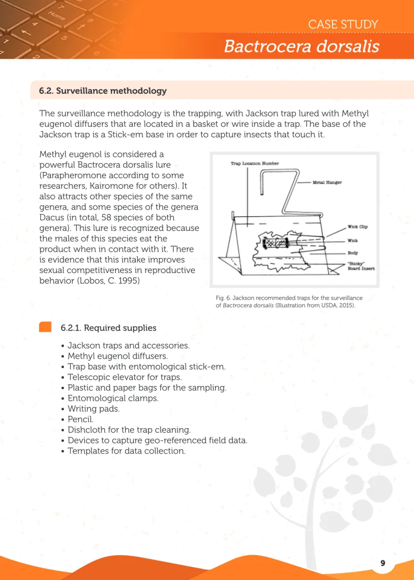
6.2. Surveillance methodology
The surveillance methodology is the trapping, with Jackson trap lured with Methyl eugenol diffusers that are located in a basket or wire inside a trap. The base of the Jackson trap is a Stick-em base in order to capture insects that touch it.
Methyl eugenol is considered a powerful Bactrocera dorsalis lure (Parapheromone according to some researchers, Kairomone for others). It also attracts other species of the same genera, and some species of the genera Dacus (in total, 58 species of both
genera). This lure is recognized because the males of this species eat the
product when in contact with it. There is evidence that this intake improves sexual competitiveness in reproductive behavior (Lobos, C. 1995)
Fig. 6. Jackson recommended traps for the surveillance of Bactrocera dorsalis (Illustration from USDA, 2015).
6.2.1. Required supplies
• Jackson traps and accessories. • Methyl eugenol diffusers.
• Trap base with entomological stick-em. • Telescopic elevator for traps.
• Plastic and paper bags for the sampling. • Entomological clamps.
• Writing pads. • Pencil.
• Dishcloth for the trap cleaning.
• Devices to capture geo-referenced field data. • Templates for data collection.
6.2.2. Trap density
The density implemented is 1 to 3 traps per selected surveillance site. The traps should be separated from one another for more than 50 meters.
In order to improve the sensibility of the system, these traps should be relocated in a radius of 200 meters from the original place where they were located.
6.2.3. Trap codification
The traps should be identified with a code that includes:
• Two (2) letters for the type of trap: JM means Jackson trap with Methyl eugenol.
• Two (2) numbers that correspond to each region.
• Three (3) numbers that correspond to the serial numbers per region. Code example: JM-02-150
The code should be written in permanent ink, in a visible part of the trap.
6.2.4 Trap services
The traps should be surveyed biweekly and during the fruiting season. And one month before the change of fruit color, the visit frequency should be weekly. In each survey, the trap information sheet at the bottom of the trap should be completed, with the date, name and signature.
The surveys and maintenance, reloading, cleaning activities made in each tramp, should include:
• Reloading the Methyl eugenol diffuser every 30 days.
• Checking the sticky base area for the possible presence of target pests. • It is possible to reuse the sticky base, without pest captures and
ensuring its sticky strength. In case of deterioration, it is replaced with a new basement.
• If any suspected Tephritidae is captured, all the basement area should be submitted for a proper diagnosis.
• The trap change should be done every three months depending on its general conditions.
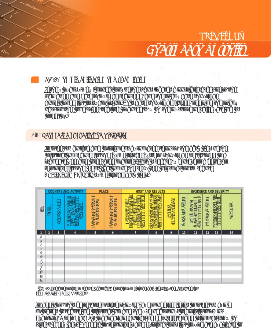
COUNTRY AND ACTIVITY PLACE HOST AND RESULTS INCIDENCE AND SEVERITY
Item
Countr
y
Date (dd/mm/aaaa) Actividad de Vigilancia Inspección, muestreo, trampeo, otro _______ (especificar)
Coordenadas geográficas decimales: LA
TITUD
Coordenadas geográficas decimales: LONGITUD Hospedante (Citrus sinensis, Citrus reticulata, Citrus unshiu, Citrus aurantifolia, Or
yza sativa,
otro_______ (especificar) Tipo de Predio (Comer
cial,
vivero, traspatio, aislado, otro________(especificar)
Resultado
(Ausente o Presente) Incidencia encontrada Descripción de la
incidencia evaluada(% u otro______ (especificar) Severidad encontrada Severidad (Grados u otro ________(especificar)
Obser vación 1 2 3 4 5 6 7 8 9 10 11 12 13 14 1 2 3 4 5 6 7 8 9 10 11 12
In addition, this general template should have modeled fields in order to avoid mistakes in recording information and the use of computing platforms. For example, Open Data Kit is capable of collecting geo-referenced information with Android devices. The details, templates and explanations for its use are available in the ODK folder in the link: https://goo.gl/WYFe6a.
Fig. 7 - General template to record Bactrocera dorsalis surveillance activities. Source: Prepared for STDF/PG/502 COSAVE Project.
6.2.5. Sample collection and submission
If the visual survey (inspection) of the traps locates a possible target pest, the trap code and date should be recorded, and the sticky base should be
conditioned for its submission. This base should be folded, keeping the sticky part on the inner side, sealing its borders, with the purpose of safeguarding its integrity.
6.3. Recording surveillance activities
In order to collate and implement automated reports, the activities of the information record for the Surveillance System should be performed in a standardized and integrated manner. In this regard, we present a general template for the identification of the required information to record
7.
COMMUNICATION
8.
AUDIT
It is important to produce reports with the results of the various level of decision making.
6.4. Biosafety
To achieve biosecurity in surveillance activities, it is necessary to include:
• The handling of traps should be done with gloves to avoid contaminating the inside of the trap or nearby locations.
• Lure diffusers should be properly identified and kept sealed in their original bags.
• Any waste material should follow NPPO waste recommendations.
Through the central coordination, each NPPO will perform auditing activities at any stage of the process, analyzing the data in the system, and monitoring the quality of the field tasks performance, among others.
9.
REFERENCES
CABI, 2017. Crop Protection Compendium. Online database. Wallingford, Reino Unido.
Costa P., Holtz V. 2011. Impacto das mudancas climáticas globais sobre a distribuicao geográfica da soja Brs valiosa RR no Brasil central. Anais do IX Seminário de Iniciação Científica, VI Jornada de Pesquisa e Pós-Graduação e Semana Nacional de Ciência e Tecnologia. Universidade Estadual de Goiás. Available on January 5, 2018.
EPPO, 1996. Quarantine Pests for Europe. Bactrocera dorsalis. European and Mediterranean Plant Protection Organization (EPPO), P Scott, CAB International. Available on October 27, 2017, at:
10.
ANNEXES
Annex 1. Data sheet of the pest
Annex 2. Modeling for Bactrocera dorsalis
Lobos, C. 1995. “Guía para la Detección de Moscas de la Fruta. Diptera:Tephritidae.” Ministerio de Agricultura de Chile, Servicio Agrícola y Ganadero. Departamento de Protección Agrícola, Proyecto Moscas de la Fruta. Chile.
Morales N., Fernandez I., Baca-Gonzales V. 2017. MaxEnt's parameter configuration and small samples: are we paying attention to recommendations? A systematic review. PeerJ 5:e3093; DOI 10.7717/peerj.3093. Available on October 27, 2017, at: https://peerj.com/articles/3093/
USDA 2015. National Exotic Fruit Fly Detection Trapping Guidelines. Available on October 27, 2017, at:
https://www.aphis.usda.gov/plant_health/plant_pest_info/fruit_flies/downloads/frui tfly-trapping-guidelines.pdf
Wang R, Li Q, He S, Liu Y, Wang M, Jiang G. 2018. Modeling and mapping the current and future distribution of Pseudomonas syringae pv. actinidiae under climate change in China. PLoS ONE 13(2): e0192153. Available on February 26, 2018, at: https://doi.org/10.1371/journal.pone.0192153
ANNEX 1
DATA SHEET OF THE PEST
Bactrocera dorsalis (Hendel, 1912)
Synonyms
Bactrocera (Bactrocera) dorsalis Drew & Hancock, 1994; Bactrocera (Bactrocera) invadens Drew et al., 2005; Bactrocera (Bactrocera) papayae Drew & Hancock, 1994; Bactrocera (Bactrocera) philippinensis Drew & Hancock, 1974; Bactrocera (Bactrocera) variabilis Lin & Wang; Bactrocera ferruginea Bezzi, 1913; Bactrocera invadens Drew, Tsuruta & White; Bactrocera papayae Drew & Hancock; Bactrocera philippinensis; Chaetodacus ferrugineus Bezzi, 1916; Chaetodacus ferrugineus dorsalis Bezzi, 1916; Chaetodacus ferrugineus var. dorsalis Hendel, 1915;
Chaetodacus ferrugineus var. okinawanus Shiraki, 1933; Dacus (Bactrocera) dorsalis Hardy, 1977; Dacus (Bactrocera) semifemoralis Tseng et al., 1992; Dacus
(Bactrocera) vilanensis Tseng et al., 1992; Dacus (Strumeta) dorsalis Hardy & Adachi, 1956; Dacus dorsalis Hendel, 1912; Dacus ferrugineus (Fabricius, 1805); Musca ferruginea Fabricius, 1794, preocc. ; Strumeta dorsalis Hering, 1956; Strumeta dorsalis okinawa Shiraki, 1968; Strumeta ferruginea Hering, 1956. Taxonomic rank Phylum: Artropoda Class: Insecta Order: Diptera Family: Tephritidae Genus: Bactrocera
Species: Bactrocera dorsalis (Hendel, 1912) Common names
Mosca oriental de la fruta (Spanish), mosca oriental das frutas (Portuguese),
oriental fruit fly (English), mango fly (English), mouche orientale des arbres fruitiers (French), Mouche des fruits asiatique (French), orientalische fruchtfliege (German). Hosts
With over 300 species of commercial/edible and wild hosts, including: Annona cherimola, Capsicum annuum, Capsicum frutescens, Carica papaya, Citrullus lanatus, Citrus aurantifolia, Citrus aurantium, Citrus limon, Citrus reticulata, Citrus sinensis, Coffea arabica, Coffea canephora, Cucumis melo, Cucurbita maxima, Cucurbita pepo, Malus domestica, Mangifera indica, Musa spp., Passiflora edulis,
Geographic distribution:
America: United States (Hawaii),
Asia: Bangladesh, Bhutan, Cambodia, China, Hong Kong, India, Laos, Malaysia, Myanmar, Nepal, Pakistan, Philippines, Singapore, Sri Lanka, Taiwan, Thailand, Vietnam
Africa: Angola, Cameroon, Congo, Ivory Coast, Ethiopia, Gabon, Ghana, Kenya, Mali, Nigeria, Senegal, South Africa, Sudan, Tanzania, Togo, Zambia, Zimbabwe (CABI, 2017).
Bactrocera dorsalis is a not present quarantine pest in COSAVE region.
Biology:
Egg to adult development of this pest at an optimum temperature of 80°F and a relative humidity of 70 percent takes approximately 22 days. The adult usually
becomes sexually mature 8 to 12 days after emergence. The minimum period of time for one generation is approximately 30 days. A mated female Bactrocera dorsalis may oviposit as many as 136 eggs per day, usually about 10 per oviposition site (USDA, 2015). Under optimum conditions, a female can lay more than 3,000 eggs during her lifetime, but under field conditions from 1,200 to 1,500 eggs per female is considered to be the usual production (Weems & Heppner, 2017). Eggs may take only 24 hours to hatch, but at cooler temperatures, they may take up to 20 days. The larval stage may last from 6 to 35 days depending on the temperature. At optimum temperatures, the larval stage can be as short as 6 to 7 days. Third instar larvae can exit fruit by a
flipping motion before or after the fruit drops to the ground. They then pupate 2-5 cm below the soil surface. Soil conditions may compel the larvae to move up to 90 cm away from fallen fruit in search of a suitable pupation site. The pupal stage usually takes 10 to 12 days to complete. This can be extended to 120 days by extremely cool temperatures. Bactrocera dorsalis usually overwinters in this stage. Newly emerged females normally require about 8-12 days to mature before they can begin to oviposit. Adults usually live for about 1 to 3 months but have survived a year in cool mountain localities. The species has been able to survive frosts and slight snowfall (USDA, 2015). The adults are best able to survive low temperatures, with a normal torpor threshold of 7°C, dropping as low as 2°C in winter (EPPO, 1996). Morphology of the pest:
The adult, which is noticeably larger than a house fly, has a body length of about 8.0 mm; the wing is about 7.3 mm in length and is mostly hyaline. The color of the fly is very variable, but there are prominent yellow and dark brown to black markings on the thorax. Generally, the abdomen has two horizontal black stripes and a
longitudinal median stripe extending from the base of the third segment to the apex of the abdomen. These markings may form a T-shaped pattern, but the pattern varies considerably (Weems H.V., Heppner J.B. 2017).
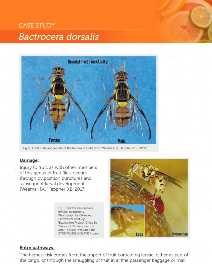
Fig. 8. Adult male and female of Bactrocera dorsalis (from Weems H.V., Heppner J.B., 2017).
Damage:
Injury to fruit, as with other members of this genus of fruit flies, occurs through oviposition punctures and subsequent larval development (Weems H.V., Heppner J.B. 2017).
Fig. 9. Bactrocera dorsalis female, ovipositing. Photograph by Okinawa Prefectural Fruit Fly Eradication Project Office in “Weems H.V., Heppner J.B. 2017”. Source: Prepared for STDF/PG/502 COSAVE Project.
Entry pathways:
The highest risk comes from the import of fruit containing larvae, either as part of the cargo, or through the smuggling of fruit in airline passenger baggage or mail. In New Zealand records 7-33 interceptions of fruit flies per year in cargo and 10-28 per year in passenger baggage (CABI, 2017). When forced, such as flying over water, movement can be as much as 40 miles. There are normally two daily peaks
Survey (inspection) and detection:
The surveillance method includes the use of Jackson traps with a diffuser of Methyl eugenol as a lure. The diffuser is held with a small basket or a wire inside the trap. The base of the Jackson trap is a sticky floor with stick-em in order to capture the insects that touch it.
The adult, which is noticeably larger than a house fly, has a body length of about 8.0 mm; the wing is about 7.3 mm in length and is mostly hyaline. The color of the fly is very variable, but there are prominent yellow and dark brown to black
markings on the thorax. Generally, the abdomen has two horizontal black stripes and a longitudinal median stripe extending from the base of the third segment to the apex of the abdomen. These markings may form a T-shaped pattern, but the pattern varies considerably. The ovipositor is very slender and sharply pointed (Weems & Heppner, 2017).
Pest impact:
Oriental fruit fly (Bactrocera dorsalis complex; Bactrocera papayae, Bactrocera philippinensis, Bactrocera invadens, and others) is one of the world's most destructive pests of soft fruits, was introduced into the Hawaiian Islands about 1945, and by 1948 had increased to high population numbers. Pakistan recorded a 70 percent infestation of peaches and pears in one area. In a second area 50-80 percent of loquat, apricot, guava, and, fig crops (USDA, 2015).
B. dorsalis is one of the five most important pests in South East Asia (EPPO, 1996). B. dorsalis is a very serious pest of a wide variety of fruits and vegetables, and damage levels can be anything up to 100% of unprotected fruit (CABI, 2017). Pest control and mitigation measures:
• Regulatory control in international trade, involving: fumigation, heat treatment (hot vapor or hot water), cold treatments, insecticidal dipping, or irradiation (CABI, 2017).
• Fruit wrapping, as a simple physical barrier to oviposition (CABI, 2017). • Removal and destruction of fallen fruit. Destruction can be by burning,
deep burrowing, feeding pigs, or placement in dark-colored plastic bags in the sun (CABI, 2017).
• A bait spray of a suitable insecticide (e.g. malathion, spinosad, fipronil) mixed with a protein bait (CABI, 2017).
• Sterile insect technique (CABI, 2017).
• Male suppression with methyl eugenol (4-allyl-1,2-dimethoxybenzene) (CABI, 2017).
• Early warning systems with a grid of methyl eugenol and cue-lure traps, at least in high-risk areas (ports and airports) (CABI, 2017).
ANNEX 2
Modeling for Bactrocera dorsalis
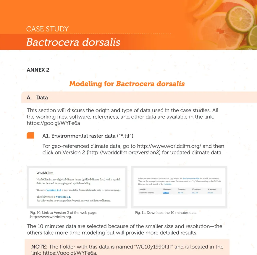
A. Data
This section will discuss the origin and type of data used in the case studies. All the working files, software, references, and other data are available in the link: https://goo.gl/WYFe6a
A1. Environmental raster data (“*.tif”)
For geo-referenced climate data, go to http://www.worldclim.org/ and then click on Version 2 (http://worldclim.org/version2) for updated climate data.
Fig. 10. Link to Version 2 of the web page: http://www.wordclim.org.
Fig. 11. Download the 10 minutes data.
NOTE: The ffolder with this data is named “WC10y1990tiff” and is located in the link: https://goo.gl/WYFe6a.
NOTE: The available variables are: BIO1 = Annual Mean Temperature, BIO2 = Mean Diurnal Range (Mean of monthly (max temp - min temp)), BIO3 = Isothermality (BIO2/BIO7) (* 100), BIO4 = Temperature Seasonality (standard deviation *100), BIO5 = Max Temperature of Warmest Month, BIO6 = Min Temperature of Coldest Month, BIO7 = Temperature Annual Range
(BIO5-BIO6), BIO8 = Mean Temperature of Wettest Quarter, BIO9 = Mean Temperature of Driest Quarter, BIO10 = Mean Temperature of Warmest Quarter, BIO11 = Mean Temperature of Coldest Quarter, BIO12 = Annual Precipitation, BIO13 = Precipitation of Wettest Month, BIO14 = Precipitation of Driest Month, BIO15 = The 10 minutes data are selected because of the smaller size and resolution—the others take more time modeling but will provide more detailed results.
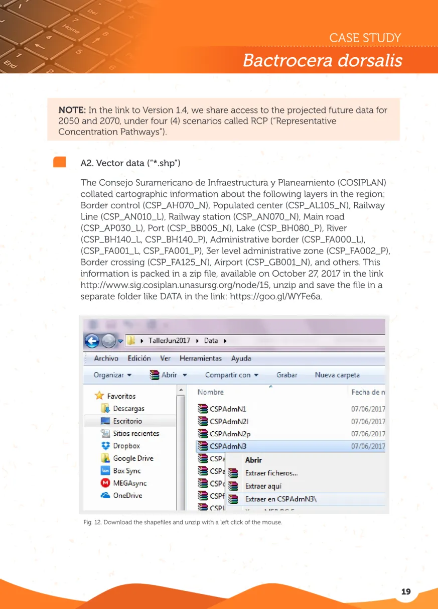
NOTE: In the link to Version 1.4, we share access to the projected future data for 2050 and 2070, under four (4) scenarios called RCP (“Representative
Concentration Pathways”).
Fig. 12. Download the shapefiles and unzip with a left click of the mouse.
A2. Vector data (“*.shp”)
The Consejo Suramericano de Infraestructura y Planeamiento (COSIPLAN) collated cartographic information about the following layers in the region: Border control (CSP_AH070_N), Populated center (CSP_AL105_N), Railway Line (CSP_AN010_L), Railway station (CSP_AN070_N), Main road
(CSP_AP030_L), Port (CSP_BB005_N), Lake (CSP_BH080_P), River (CSP_BH140_L, CSP_BH140_P), Administrative border (CSP_FA000_L), (CSP_FA001_L, CSP_FA001_P), 3er level administrative zone (CSP_FA002_P), Border crossing (CSP_FA125_N), Airport (CSP_GB001_N), and others. This information is packed in a zip file, available on October 27, 2017 in the link http://www.sig.cosiplan.unasursg.org/node/15, unzip and save the file in a separate folder like DATA in the link: https://goo.gl/WYFe6a.
B. Software B1. QGIS
QGIS (anteriormente llamado también Quantum GIS) es un Sistema de Información Geográfica (SIG) de código libre para plataformas GNU/Linux, Unix, Mac OS y Microsoft, soporta numerosos formatos y funcionalidades de datos vector, datos raster y bases de datos. Además, cuenta con extensiones específicas, disponibles en <http://plugins.qgis.org/plugins/ >, que lo hace
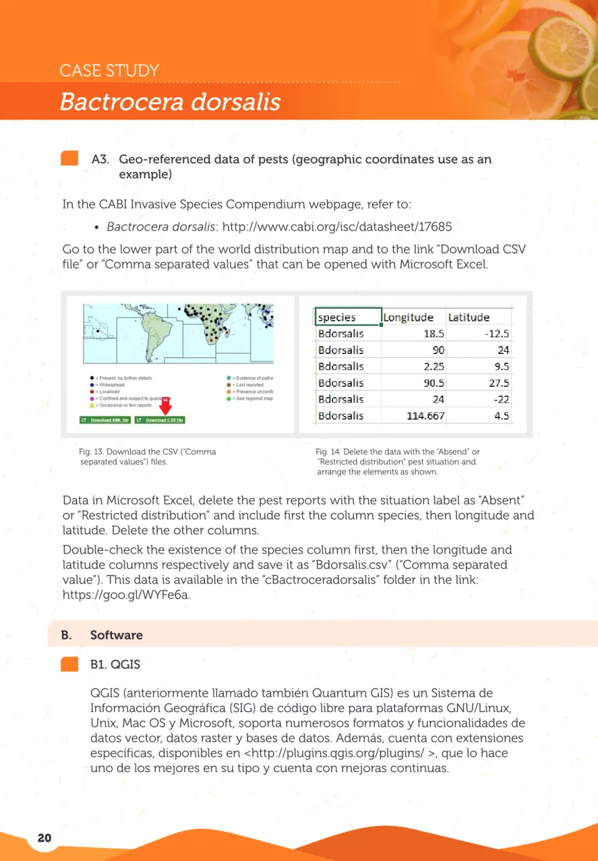
A3. Geo-referenced data of pests (geographic coordinates use as an example)
In the CABI Invasive Species Compendium webpage, refer to:
• Bactrocera dorsalis: http://www.cabi.org/isc/datasheet/17685
Go to the lower part of the world distribution map and to the link “Download CSV file” or “Comma separated values” that can be opened with Microsoft Excel.
Fig. 13. Download the CSV (“Comma separated values”) files.
Fig. 14. Delete the data with the “Absend” or “Restricted distribution” pest situation and arrange the elements as shown.
Data in Microsoft Excel, delete the pest reports with the situation label as “Absent” or “Restricted distribution” and include first the column species, then longitude and latitude. Delete the other columns.
Double-check the existence of the species column first, then the longitude and latitude columns respectively and save it as “Bdorsalis.csv” (“Comma separated value”). This data is available in the “cBactroceradorsalis” folder in the link: https://goo.gl/WYFe6a.
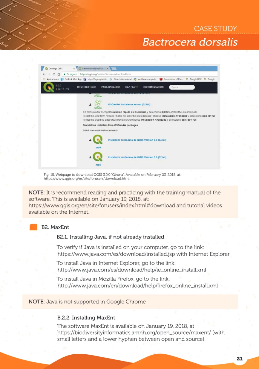
Fig. 15. Webpage to download QGIS 3.0.0 “Girona”. Available on February 23, 2018, at: https://www.qgis.org/es/site/forusers/download.html
NOTE: It is recommend reading and practicing with the training manual of the software. This is available on January 19, 2018, at:
https://www.qgis.org/en/site/forusers/index.html#download and tutorial videos available on the Internet.
B2. MaxEnt
B2.1. Installing Java, if not already installed
To verify if Java is installed on your computer, go to the link:
https://www.java.com/es/download/installed.jsp with Internet Explorer To install Java in Internet Explorer, go to the link:
http://www.java.com/es/download/help/ie_online_install.xml To install Java in Mozilla Firefox, go to the link:
http://www.java.com/en/download/help/firefox_online_install.xml NOTE: Java is not supported in Google Chrome
B.2.2. Installing MaxEnt
The software MaxEnt is available on January 19, 2018, at
https://biodiversityinformatics.amnh.org/open_source/maxent/ (with small letters and a lower hyphen between open and source).
Fig. 18. Search for the DATA folder and unzip *.shp files. Fig. 19. Locate the shapefile (*.shp) and click on “Open”.
NOTE: Check the right lower edge for the CRS “Coordinate Reference System” in World Geodetic System 1984 - WGS84 with the code: 4326, recommended because
Fig. 16. Link to download MaxEnt software and optional requirement of user personal data.
Fig. 17. Download Version 3.4.1. and the cited reference of the MaxEnt software.
C. Activities:
C1. Opening a shapefile (or vector layer) and converting the raster data files (“*.tiff” to “*.asc”) for the use of MaxEnt software in the modeling.
C1.1. Opening a shapefile in QGIS:
A shapefile has (at least) three files with the same name but with a different extension. The file with the SHP (“*.shp”) extension is the main file and includes spatial features.
Open the QGIS with the short option: add vector layer (left side) or the “Layer” tab, as shown in the below figure:
Figura 20. Correspondencia aproximada entre grados y
kilómetros en el Ecuador (de: Sheldeman y van Zonneveld, 2011).
For the conversion, select the “Raster/Conversion/Translate” option, as shown in Fig. 20, in the box “Input Layer” select each file “*.tif” and in the box “Output file” the location of the “*.asc” files in a folder like WC10y1990asc (not the
WC10y1990tiff folder) and select the Spatial Reference System (SRS) EPSG:4326, as illustrated in Fig. 23.
Fig. 22. Command “Translate” to convert raster “*.tif” files to “*.asc”.
Fig. 23. Details of the conversion, specifying the “*.asc” extension.
Approximate size of geographic units (at the Equator), rounded (in km)
Degrees 1 degree 10 minutes 5 minutes 2.5 minutes 30 seconds Size 111 km 18 km 9 km 5 km 1 km
C.1.2. Converting raster data (“*.tif” to “*.asc”):
A raster is a set of pixels with the same size; each pixel has a different value for a variable (including
temperature, type of soil). The size of the pixel is called “resolution”, and its selection depends on the
geographical scope and the objective of the project.
To open the raster file, choose the “Add Raster Layer” option on the left side, as shown in the figure below. Locate, select and open files like “bio10m01.tif” from the “WC10y1990tiff” file.
Fig. 21. Command to open raster (“*.tif”) files, indicated with the red arrows in the Layer/Add layer/Add Raster Layer tab.
Check the “*.asc” extension in the output file and the selection of the Spatial Reference System.
Repeat the same procedure with the 19 layers of the bioclimatic variables
downloaded in section A1, which are available in the link: https://goo.gl/WYFe6a and the WC10y1990tiff folder.
NOTA: The raster “*.asc” files are also available in the WC10y1990asc folder in the link: https://goo.gl/WYFe6a.
C2. Using MaxEnt for the modeling.
To open the MaxEnt software, click on the “maxent.jar” file. Then open the “Settings” option, select “Basic” and include the standard option and the box “Random test percentage” write 25 for an additional software test with 25% of the samples. Then close the window.
Fig. 24. In “Settings” and “Basic”, include the standard options, as illustrated here.
Fig. 25. Main screen where geo-referenced data and bioclimatic variables are included in “*.asc” format.
In the main screen, in the samples option, select the “*.csv” (“Comma separated values” not “*.xls”) file with the geo-referenced pest data. This was discussed in section A3. Next, select "Auto features", "Create response curves", "Make pictures of predictions", "Do jackknife to measure variable importance", "Logistic format" and "asc file type", and select a folder for the output of the files, thus ordering a complete modeling, with figures like “Do jackknife” that visually describe the contribution of each bioclimatic variable to the final model. In the other part with the environmental layers option, choose the folder with the converted variables to the “*. asc” format, i.e. a raster file like the one described in section A1.
For practical purposes, record warning messages like “Unused field” or “Missing environmental data” and click “Ok”.
Fig. 26. Record messages like “Unused field” o “Missing environmental data”.
Fig. 27. After checking the repetition of messages, you can select the “Suppress similar visual warnings” option.
The results of the environmental modeling are available in the Bdorsalis.html file, which can be opened with any web browser. The raster file of the map is available in the Bdorsalis.asc file, as illustrated in the figure below.
Fig. 28. File with the results of the MaxEnt modeling.
Fig. 29. Opening the “*.html” file with the modeling. The “*.asc” file is a raster, as those described in section A1.
C3. Open a map in geographical coordinates, creating a 100 Km reference grid and a centroid in each grid.
Develop a grid with a reference size of 100 Km or 0.9 decimal degrees, based on the equivalences of grades and kilometers from Sheldeman X. & van Zonneveld M. 2011, shown in Fig. 20.
First, open a shape vector layer from COSIPLAN (http://www.sig.cosiplan.unasursg.org/node/15).
Fig. 30. Open a reference vector layer with the “*.shp” extension.
Fig. 31. Find the “Create Grid” function in the “Processing toolbox” (see the note below) and click it.
NOTE: If the “Processing toolbox”.is not available, please select it in tab “View”, “Panels” and then “Processing toolbox”.
In the “Grid type” choose the “Rectangle (polygon)” option in the “Grid extent” choose “select extent on canvas” dragging the mouse on the map to create the grid. Complete “Vertical spacing” and “Horizontal spacing” with the 0.9 data. Check that EPSG 4326 – WGS84 is in “Grid CRS” and provide a route to save the grid file. Finally, click on “Run in Background” as illustrated in the figure below.
Fig. 34. To make the grid transparent, select “Single symbol”, “Fill Style”, then “No brush”.
Fig. 35. To obtain centroids in each grid, find the “Centroids” function (“Vector geometry” set) in “Processing Toolbox”.
In the “Layers” panel, you can change the grid file appearance and its location in the map with a right click on its name. To make it transparent, select “Options”, “Style”, “Single symbol”, “Fill”, “Simple fill”, and in “Fill style” select “No Brush”. Front or background movement on the map is commanded with a change in file position in the “Layers” panel.
NOTE: If the Processing toolbox is not available, please select it in tab “View”, “Panels” and then “Processing toolbox”.
Using this vector “*.shp” file of centroids, you can extract values from the modeling.
Fig. 36. Details of the use of the “Centroids” function (“Vector geometry”).
C4. Integrating information with QGIS
C4.1. Develop a vector shapefile with crop production information in the administrative geopolitical units of each country:
First, open the file for the second level administrative geopolitical unit "CSP_FA001_P.shp" downloaded in section A2. Then with the right click on the file, select “Open attribute table” and “Toggle edition tool” by clicking on the pencil in the top left corner of the screen.
Fig. 38. Open the “CSP_FA001_P.shp” shapefile downloaded in section A2 and with a right click on the “Open attribute table” option.
Fig. 39. Select the “Conmutar edición” with the pencil in the top left corner of the screen.
The vector file “CSP_FA001_P.shp” can include an additional column, where you can record the host area or a host risk index value like 0, 1 or 2 (2 as the
maximum value). The host area can be also a “Whole number (Integer)” having as many digits as the largest production area record. Both files are available in the https://goo.gl/WYFe6a folder.
C4.2. Converting a vector shapefile in a raster.
In order to integrate the host risk index, first convert the vector “*.shp” file to raster with a function in the tap “Raster”, “Conversions” and then “Rasterize (vector to raster)”. To do this, use the column with the host risk index for the value of the raster. The illustration of this function is shown in the figure below.
For a better view of model raster values, with a right click on the layer, open the “Properties” then “Style”, “Singleband pseudocolor” with the “Spectral” option. Include the modification of the label as HIGH, MEDIUM or LOW, as illustrated in the figure below.
Fig. 42. With the “Rasterize” function, convert the “CSP_FA001_P.shp” file using the host risk index as a value.
Fig. 43. For a better presentation of the bioclimatic risk model, change the properties with a right click on the layer.
Moreover, it is possible to integrate the environmental risk with the host risk index or others with the “Raster calculator” function, which develops math between raster layers. With this tool, you can also integrate information on land cover or Normalized Vegetation Index (NDVI), which are raster files too. When raster layers are multiplied, the grids with a lower value are integrated with the zero (0) value, while higher categories are integrated with maximum values, as shown in Table 3.
C4.3. Reclassifying the raster of the model for its integration. Similarly to the host risk index, index 0, 1 or 2 is required in the environmental modeling. For this purpose, use the “Reclassify values
(simple)” function from SAGA (System for Automated Geoscientific Analysis) in the “Processing toolbox” on the right side of QGIS. In the function, select the “Fixed Table 3x3” option with the values 0, 1 or 2. These details are illustrated in the figures below.
Fig. 44. Location of the “Reclassify values (simple)” function in SAGA.
Fig. 45. Details of the “Reclassify values” function and the “Fix table 3x3”.
Table 3. Integrating raster files with the reclassification of the value in the grid and the multiplication function in the “Raster calculator”.
RASTER
INTEGRATION LOW INDEX B = 0 MEDIUM INDEXB = 1 HIGH INDEX B = 2 LOW INDEX
A = 0 LOW = 0 LOW = 0 LOW = 0
MEDIUM INDEX
A = 1 LOW = 0 MEDIUM = 1 MEDIUM = 2
HIGH INDEX
The figure below illustrates the use and results of the “Raster calculator” function:
Fig. 46. Details in the “Raster calculator” function for the integration of raster layers.
Fig. 47. Regional Risk map. Higher risk in red, medium risk in yellow and lower risk in light blue. Scale 1:45,000,000.
C4.4. Obtaining risk values with a vector shapefile
Open the ports layer “CSP_BB005_N.shp” and the airports layer
“CSP_GB001_N.shp” as explained in section A2, to extract risk values to a vector (point) layer. You can also change their names with the right click. This vector file can also be a centroid in a grid like that in C3.
To include geographical coordinates, make a right click on the vector file and select “Open attributes table”. Then use the “Field calculator” as shown with the red arrow in the figure below and the “Geometry” option selecting $x for the field “longitude” and $y for the field “latitude”. It is important to check that the format of the field is “Decimal number (real)” and with 5 decimals of precision.
In the “Processing toolbox” on the right side, find the “v.sample” function and obtain raster values from the results of sections C2 or C4.3, as illustrated in the figures below.
This layer “Sampled” can be integrated with another vector shapefile, like the 100 km grid that created the centroids. For this, find the “Join attributes by location” function in the “Processing toolbox”. Select the “Sampled” layers and the “Grid” shapefile and save it, as illustrated in the figure below.
Fig. 48. With a right click on the vector shapefile, open the “Attributes table” and the “Field calculator”, as indicated by the red arrow.
Fig. 49. Create a field called “longitude” as a “Decimal number (real)” with 5 decimals and the “Geometry” function, then “$x” and similarly with “$y” for the “latitude”.
Fig. 50. Sampling risk values with a vector shapefile in a new file “Sampled” in a new route for the file.
Fig. 51. The developed shapefile has points and values that can be graphically shown, changing layer properties.
Figura 54. Con la función Propiedades de la capa se cambia la presentación de estilo en la capa de aeropuertos o puertos
Figura N° 55. Presentación personalizada de la capa de aeropuertos en concordancia con el valor de riesgo (riesgo: alto en rojo y de mayor tamaño, medio de amarillo y bajo en celeste de tamaño pequeño)
The resulting vector shapefile layer contains origin and modeled risk information. This information can be exported with the right click on the layer, as illustrated in the figures below:
This integrated information can be shown in a map, selecting with a right click the “Layer properties”, “Style” and “Categorize” in reference to the values of the modeling, as shown in the figures below.
It is also feasible to integrate other geo-referenced information, like the river layer “CSP_BH140_L.shp”, available in https://goo.gl/WYFe6a using the
“Intersection” function in the “Vector” tab and “Geoprocessing tools” group.
Fig. 56. To collect the information in another format, you can select the layer with a right click and choose “Save as”.
Fig. 57. Save the information in CSV (“Comma separated values”) format, which can be opened in Microsoft Excel.
NOTE: All this case study information is available in the Bactrocera dorsalis folder in the link: https://goo.gl/WYFe6a.
Fig. 58. Extracted raster values and the airport identification, for further analysis.
In Microsoft Excel, the NPPO can assess the risk parameters in based on expert criteria. The figure below provides an example.
References
ISPM 26. Establishment of pest free areas for fruit flies (Tephritidae). 2016 Sheldeman X & van Zonneveld M. 2011. Manual de Capacitación en Análisis Espacial de Diversidad y Distribución de Plantas. Bioversity International, Rome, Italy. 186 pp. Available on October 27, 2017, at:
http://www.bioversityinternational.org/e-library/publications/detail/manual-de-capacitacion-en-analisis-espacial-de-diversidad-y-distribucion-de-plantas/ Weems H.V., Heppner J.B. 2017. Bactrocera dorsalis (Hendel) (Insecta: Diptera: Tephritidae). University of Florida, and Gary Steck, Florida Department of Agriculture and Consumer Services. Available on October 27, 2017, at: http://entnemdept.ufl.edu/creatures/fruit/tropical/oriental_fruit_fly.htm