1
Mapping the global design space of integrated
photonic components using machine learning
pattern recognition
Daniele Melati
1,†, Yuri Grinberg
2,†, Siegfried Janz
1, Pavel Cheben
1,
Jens H. Schmid
1, Alejandro Sánchez-Postigo
3and Dan-Xia Xu
1,*1
Advanced Electronics and Photonics Research Centre, National Research Council Canada, 1200 Montreal Rd., Ottawa, ON K1A 0R6, Canada
2
Digital Technologies Research Centre, National Research Council Canada, 1200 Montreal Rd., Ottawa, ON K1A 0R6, Canada
3
Universidad de Málaga, Departamento de Ingeniería de Comunicaciones, ETSI Telecomunicación, Campus de Teatinos s/n, 29071 Málaga, Spain
*e-mail: [email protected]
†
These authors contributed equally to this work.
1. Uncertainty analysis with polynomial chaos expansion
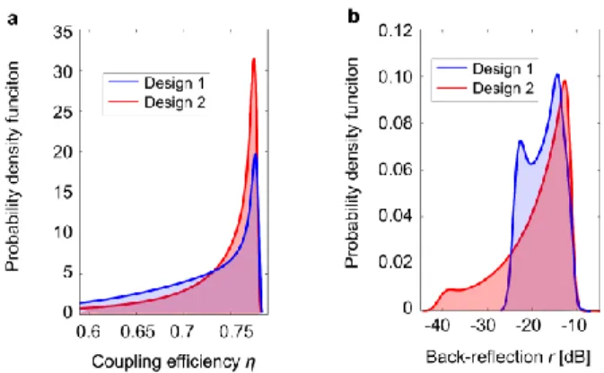
In order to verify the results of the uncertainty analysis described in the manuscript, we compute the probability density functions of the coupling efficiency and back-reflections for designs 1 and 2 (see Fig. 3 in the manuscript). Width deviations δ are assumed to be normally distributed with zero mean and a standard deviation of 5 nm2. Probability density functions are efficiently calculated using 2D-FDTD in combination with a polynomial chaos model3,4. Eighty different values for δ are sampled according to their distribution. Corresponding designs are generated and simulated with 2D-FDTD to obtain the coupling efficiency and back-reflection for each of them. For both quantities a corresponding stochastic surrogate model describing their dependence on δ (polynomial chaos model) is realized with fifteenth-order Hermite polynomials as the orthonormal basis. The coefficients of the polynomials are estimated from the 80 simulations with a compressed sensing technique solving a corresponding basis pursuit denoise problem with the freely available spgl1 solver5. Details on how to compute the polynomial chaos surrogate model can be found in ref 4. Finally, the two probability density functions are obtained with a standard Monte Carlo simulation by sampling the surrogate models 5000 times (which only takes few seconds) and using a Gaussian kernel density estimator.
Although the polynomial chaos model allows to accurately compute the required stochastic properties with a limited number of 2D-FDTD simulations, the previous analysis based on PCA is of fundamental importance to first identify the possible design candidates deserving further analysis. Regarding coupling efficiency (Fig. 1a), the probability density functions of both designs are right-bounded by the value obtained without considering uncertainty (about 0.76 in both cases) but design 1 shows a longer tail towards lower values of η. This means that the probability to obtain a high coupling efficiency is lower compared to design 2 and therefore a lower fabrication yield is expected for design 1. As shown in Fig.
2
1b, also the lower value of the two back-reflection probability density functions is limited by the performance obtained without uncertainty. As discussed in the manuscript, without uncertainty design 2 has substantially smaller back-reflections (smaller than -40 dB) but as predicted by the map of Fig. 4b in the manuscript the region of low back-reflection is highly localized, and back-reflection quickly grows when width variations are introduced (longer tail of the function). In contrast, the minimum back-reflection achievable by design 1 is much higher but its variability is considerably smaller, as demonstrated by the narrower probability density function. In both cases backreflections do not exceed -10 dB (worst-case-scenario) with the considered uncertainty.
2. Evaluating the generality of hyperplanes
The hyperplanes described in the manuscript provide a comprehensive characterization of the grating design space for C band. It is natural to question whether this finding can be extended to other scenarios. The optical communication O band (1260 nm to 1360 nm) is another important wavelength range particularly for data centers6. We thus apply the approach described in the manuscript to design vertical grating couplers at a wavelength λ = 1310 nm, using the same grating structure and adjusting material indices (3.50 and 1.45 for silicon and silica, respectively) and SMF-28 fiber mode (MFD 9.2 μm) for the reduced wavelength. We execute the optimization stage until it generates 5 different designs with a coupling efficiency of η > 0.75. The highest value was found to be η = 0.77. Following the analysis for λ = 1550 nm, 5 designs are speculated to be sufficient to define the reduced parameter space through PCA as long as the approximation errors are small. Indeed, our results confirm that the sub-space of high performance designs can be accurately represented on a 2-D hyperplane incurring an average approximation error smaller than 2 nm.
Fig. 1 Tolerance to fabrication uncertainty. Probability density functions for (a) coupling efficiency and (b) back-reflections for
designs 1 and 2 described in the manuscript. Design 1 shows a longer tail towards lower values of η, slightly reducing the probability to obtain a high coupling efficiency. Design 2 has a much smaller value of back-reflection that quickly grows when width variations are introduced (longer tail of the function). On the contrary, the variability of back-reflections for design 1 is considerably smaller as demonstrated by the narrower probability density function, but a reflection less than -25 dB is never obtained.
3
The vectors defining the α-β hyperplane are V1αβ = [11.50, -7.76, 32.60, 22.59, -28.46] nm, V2αβ = [11.18,
3.91, 34.07, -52.56, 0.76] nm and Cαβ = [59.40, 63.2, 50, 105.6, 238] nm (see equation (2) in the
manuscript).
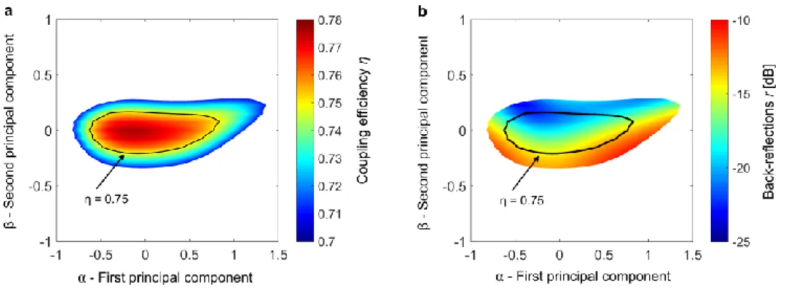
Figures 2a and 2b report the results of the exhaustive exploration of the sub-space on the α-β hyperplane limited to the region defined by η > 0.70. The same unit (100 nm per division) in α or β is used as in Figs. 3a and 3b in the manuscript. Identifying the region of top performing designs through an exhaustive brute force search in a five-dimensional space would incur an increase of several orders of magnitude in computation time, making it practically infeasible to implement.
Considering that the basic grating structure is unchanged, the sub-space of good designs looks remarkably different compared to that found for λ = 1550 nm. For the latter, good designs occupied a sub-space with approximately the same size in α and β (about 3 units, Figs. 3a and 3b). In the case for λ = 1310 nm the range allowed on α is similar (about 2 units) while a tighter choice is available along β (about 0.6 units). Nonetheless a design area with η > 0.75 can still be identified with designs ensuring similar fiber coupling efficiency but different back-reflections, ranging from -22 dB to -13 dB. Within this area the minimum feature size ranges between 30 nm and 60 nm, depending on the selected design.
References
1. Melati, D., Waqas, A., Xu, D.-X. & Melloni, A. Genetic algorithm and polynomial chaos modelling for performance optimization of photonic circuits under manufacturing variability. in Optical Fiber
Communication Conference M3I.4 (Optical Society of America, 2018). doi:10.1364/OFC.2018.M3I.4
2. Xu, D. et al. Silicon Photonic Integration Platform—Have We Found the Sweet Spot? IEEE J. Sel.
Top. Quantum Electron. 20, 189–205 (2014).
Fig. 2 Design of vertical grating couplers at λ = 1310 nm. The two maps show the coupling efficiency (a) and back-reflection (b)
across the sub-space of good designs for a grating with the same structure shown in Fig. 2a but operating at λ = 1310 nm. PCA allows again to efficiently represent the design space using a 2-D hyperplane.
4
3. Xiu, D. Fast Numerical Methods for Stochastic Computations: A Review. Commun Comput Phys 31 (2009).
4. Weng, T.-W., Melati, D., Melloni, A. & Daniel, L. Stochastic simulation and robust design optimization of integrated photonic filters. Nanophotonics 6, 299–308 (2017).
5. van den Berg, E. & Friedlander, M. Probing the Pareto Frontier for Basis Pursuit Solutions. SIAM J.
Sci. Comput. 31, 890–912 (2008).