HAL Id: hal-01817742
https://hal.archives-ouvertes.fr/hal-01817742
Submitted on 18 Jun 2018
HAL is a multi-disciplinary open access
archive for the deposit and dissemination of
sci-entific research documents, whether they are
pub-lished or not. The documents may come from
teaching and research institutions in France or
abroad, or from public or private research centers.
L’archive ouverte pluridisciplinaire HAL, est
destinée au dépôt et à la diffusion de documents
scientifiques de niveau recherche, publiés ou non,
émanant des établissements d’enseignement et de
recherche français ou étrangers, des laboratoires
publics ou privés.
A 1D Continuum Model for Beams with Pantographic
Microstructure: Asymptotic Micro-Macro Identification
and Numerical Results
Emilio Barchiesi, Francesco Dell’Isola, Marco Laudato, Luca Placidi, Pierre
Seppecher
To cite this version:
Emilio Barchiesi, Francesco Dell’Isola, Marco Laudato, Luca Placidi, Pierre Seppecher. A 1D
Con-tinuum Model for Beams with Pantographic Microstructure: Asymptotic Micro-Macro Identification
and Numerical Results. Advances in Mechanics of Microstructured Media and Structures , 87, pp
43-74, 2018, Advanced Structured Materials book series (STRUCTMAT), volume 87. �hal-01817742�
with Pantographic Microstructure:
Asymptotic Micro-Macro Identification
and Numerical Results
Emilio Barchiesi, Francesco dell’Isola, Marco Laudato, Luca Placidi and Pierre Seppecher
Abstract In the standard asymptotic micro-macro identification theory, starting from a De Saint-Venant cylinder, it is possible to prove that, in the asymptotic limit, only flexible, inextensible, beams can be obtained at the macro-level. In the present paper we address the following problem: is it possible to find a microstructure pro-ducing in the limit, after an asymptotic micro-macro identification procedure, a con-tinuum macro-model of a beam which can be both extensible and flexible? We prove that under certain hypotheses, exploiting the peculiar features of a pantographic microstructure, this is possible. Among the most remarkable features of the result-ing model we find that the deformation energy is not of second gradient type only because it depends, like in the Euler beam model, upon the Lagrangian curvature, i.e. the projection of the second gradient of the placement function upon the normal vector to the deformed line, but also because it depends upon the projection of the second gradient of the placement on the tangent vector to the deformed line, which is the elongation gradient. Thus, a richer set of boundary conditions can be prescribed
E. Barchiesi ⋅ F. dell’Isola (
✉
)Dipartimento di Ingegneria Strutturale e Geotecnica, Università degli Studi di Roma “La Sapienza”, Via Eudossiana 18, 00184 Roma, Italy
e-mail: [email protected]
E. Barchiesi ⋅ F. dell’Isola ⋅ M. Laudato ⋅ L. Placidi ⋅ P. Seppecher
International Research Center M&MoCS, Università degli Studi dell’Aquila, Via Giovanni Gronchi 18 - Zona industriale di Pile, 67100 L’Aquila, Italy
L. Placidi
Facoltà di Ingegneria, Università Telematica Internazionale UNINETTUNO, Corso Vittorio Emanuele II 39, 00186 Roma, Italy
F. dell’Isola
Dipartimento di Ingegneria Civile, Edile, Ambientale e Architettura, Università degli Studi dell’Aquila, Via Giovanni Gronchi 18 - Zona industriale di Pile, 67100 L’Aquila, Italy M. Laudato
Dipartimento di Ingegneria e Scienze dell’Informazione e Matematica, Università degli Studi dell’Aquila, Via Vetoio 1, 67100 L’Aquila, Coppito, Italy P. Seppecher
Institut de Mathématiques de Toulon, Universitè de Toulon et du Var, Avenue de l’Université, BP 132, Cedex, 83957 La Garde, France
for the pantographic beam model. Phase transition and elastic softening are exhibited as well. Using the resulting planar 1D continuum limit homogenized macro-model, by means of FEM analyses, we show some equilibrium shapes exhibiting highly non-standard features. Finally, we conceive that pantographic beams may be used as basic elements in double scale metamaterials to be designed in future.
Keywords Micro-macro identification
⋅
Asymptotic expansion⋅
Pantographic beams⋅
Continuum models1
Introduction
Customarily, the theory of nonlinear beams is either postulated by means of a suit-able least action principle in the so called “direct way” or is deduced, by means of a more or less rigorous procedure, starting from a three-dimensional elasticity theory. The first example of direct model can be found in the original paper by Euler [1]. Many epigones of Euler used this approach: a comprehensive account for this proce-dure can be found in e.g. Antman [2]. On the other hand, by following the procedure described by De Saint-Venant, one can try to identify the constitutive equation of an Euler type (1D) model in terms of the geometrical and mechanical properties, at micro-level, of the considered mechanical systems. This is done, in more mod-ern textbooks, by using a more or less standard asymptotic micro-macro identifica-tion procedure, which generalizes the one used by De Saint-Venant for bodies with cylindrical shape (see for instance [3]). It can be rigorously proven, under a series of well-precised assumptions, that only flexible and inextensible beams can be obtained [4–9]. In the present paper we address the following problem: is it possible to find a microstructure producing, at the macro level and under loads of the same order of magnitude, a beam which can be both extensible and flexible? Using an asymp-totic expansion and rescaling suitably the involved stiffnesses, we prove that a panto-graphic microstructure does induce, at the macro level, the aforementioned desired mechanical behaviour. In this paper, in an analogous fashion to that of variational asymptotic methods, and following a mathematical approach resembling that used by Piola, we have employed asymptotic expansions of kinematic descriptors directly into the postulated energy functional. Using the so obtained 1D continuum model, we show some equilibrium shapes exhibiting highly non standard features, essen-tially related to the complete dependence of the homogenized continuum energy density functional on the second gradient of the placement field. While in the stan-dard finite deformation Euler beam theory the energy functional depends only on the material curvature, i.e. the normalized projection of the second gradient of the placement on the normal vector to the current configuration, the energy functional for the nearly-inextensible pantographic beam model depends also on the projection of the second gradient of the placement on the tangent vector to the current con-figuration. Thus, the full decomposition of the second gradient of the placement is present in the latter model. Generalized continua [10–14], and in particular higher
gradient theories, see [15] or [16] for a comprehensive review, are able to describe behaviours which cannot be accounted for in classical Cauchy theories [17–24]. In the literature, several examples can be found motivating the importance of gener-alized continua: electromechanical [25] and biomechanical [26–29] applications, elasticity theory [30–35], capillary fluids analysis [36], granular micromechanics [37–39], robotic systems analysis [40,41], damage theory [42–47], and wave prop-agation analysis [48–52]. Furthermore, second gradient continuum models always appear when the considered micro-system is a pantographic structure [53–60]. A comprehensive review on the modeling of pantographic structures can be found in [61, 62]. Several results of numerical investigations can be found in [30, 63–71], while for an outline of recent experimental results we refer to [72, 73]. The work is organized in the following way. In Sect.2, we discuss the geometry of the panto-graphic beam micromechanical model. Once the general expression for the micro-model energy is given, we restrict to the quasi-inextensibility case, where small elon-gation of oblique fibers is assumed. The micro-model energy is then represented as a function of the macroscopic kinematical descriptors and the further specializa-tion to the (complete) inextensibility of the oblique fibers is considered. In Sect.3
we perform a heuristic homogenization procedure and we discuss the feature of the 1D continuum model. In particular, we show that such a homogenization procedure gives rise to a full second gradient theory. In Sect.4we show results of numerical simulations in order to better highlight some non-standard features of the nearly-inextensible pantographic beam model. Finally, in Sect.5we postulate a generalized strain energy density which includes both the quasi-inextensible pantographic beam model and the standard Euler beam theory. Euler-Lagrange equations for this gen-eralized strain energy density are derived together with the corresponding boundary conditions and the specializations to the two models are performed.
2
Discrete Micro-model
In this section we discuss the discrete micro-mechanical model which is employed throughout this paper. We begin giving a geometrical description and then we give a mechanical characterization, by choosing a deformation energy. It is a Hencky-type spring model with the geometrical arrangement of a pantographic strip. Once the energy of the micro-model is chosen in its general form, we assume a particular asymptotic behaviour for some relevant kinematic quantities, i.e. the elongation of oblique springs, as will be clear in the sequel. We consider the quasi-inextensibility case, i.e. the relative elongation of the oblique springs is small. As a further spe-cialisation, the inextensibility case is considered. Finally, after having defined a micro-macro identification, we express the energy of the micro-system in terms of macroscopic kinematic descriptors to prepare the field to the homogenization pro-cedure which will be discussed in details in the next section.
2.1 Geometry
In the spirit of [55, 59, 74], in this section we introduce a discrete-spring model (also referred to as the micro-model, since it resembles the features of a specific microstructure). The topology and features of the undeformed and deformed discrete-spring system are summarized in Figs.1and2, respectively. In the undeformed con-figuration N + 1 material particles are arranged upon a straight line at positions Pi’s,
i ∈[0; N], with a uniform spacing 𝜀. The basic i-th unit cell centered in Piis formed
by four springs joined together by a hinge placed at Pi. Between two oblique springs,
belonging to the same cell and lying on the same diagonal, a rotational spring oppos-ing to their relative rotation is placed. Rotational sproppos-ings are colored in Fig.1in blue and red.
We denote with pithe position in the deformed configuration corresponding to
position Piin the reference one. In order to completely describe the kinematics of
the micro-model we have to introduce other descriptors. At this end, the length of the oblique deformed springs, indicated with l𝛼𝛽i , is introduced, the indices𝛼 and 𝛽 belonging respectively to the sets {1, 2} and {D, S} and referring to the first and
Fig. 1 Undeformed spring system resembling the micro-structure
second diagonal and left and right, respectively. Referring to Fig.2, we consider the i-th node, notwithstanding that the same quantities can be defined for each node. We define𝛼ias the angle between the vectors pi− pi−1 and pi− pi+1, respectively. We
define as𝜗𝛼i the angle measuring the deviation of two opposite oblique springs from being collinear. In order to illustrate the definition of𝜑𝛼𝛽i , we consider the case𝛼 = 1 and𝛽 = D. The quantity 𝜑1Di is the angle between the vector pi+1− piand the upper
oblique spring hinged at pi. By means of elementary geometric considerations, we
have that
𝜗1
i = 𝛼i+ 𝜑1Di − 𝜑1Si
𝜗2
i = 𝛼i+ 𝜑2Si − 𝜑2Di , i ∈ [0; N] . (1)
In the undeformed configuration, see Fig.1, we have:
l𝛼𝛽i = √ 2 2 𝜀, 𝛼 = 1, 2 𝛽 = D, S i ∈ [0; N] 𝜗1 i = 𝜗2i = 0 ‖pi− pi−1‖ = 𝜀, i ∈ [0; N] . (2)
Considering that𝜑𝛼Di , 𝜑𝛼Si ∈ [0, 𝜋], by means of the law of cosines, we get:
𝜑1D i = cos−1 ⎛ ⎜ ⎜ ⎝ ‖pi+1− pi‖2+(l1D i )2 −(l2Si+1)2 2l1D i ‖pi+1− pi‖ ⎞ ⎟ ⎟ ⎠ 𝜑2D i = cos−1 ⎛ ⎜ ⎜ ⎝ ‖pi+1− pi‖2+(l2D i )2−( l1Si+1)2 2l2D i ‖pi+1− pi‖ ⎞ ⎟ ⎟ ⎠ 𝜑1S i = cos−1 ⎛ ⎜ ⎜ ⎝ ‖pi− pi−1‖2+(l1S i )2−( l2Di−1)2 2l1S i ‖pi− pi−1‖ ⎞ ⎟ ⎟ ⎠ 𝜑2S i = cos−1 ⎛ ⎜ ⎜ ⎝ ‖pi− pi−1‖2+ ( l2Si )2−(l1Di−1)2 2l2S i ‖pi− pi−1‖ ⎞ ⎟ ⎟ ⎠ . (3)
2.2 Mechanical Model
The micro model energy, written as a combination of the elastic energy contributions of the springs, is defined as:
= ∑ i ∑ 𝛼,𝛽 ke 𝛼𝛽,i 2 ( li𝛼𝛽− √ 2 2 𝜀 )2 +∑ i ∑ 𝛼 kf𝛼,i 2 ( 𝜗𝛼 i )2+ +∑ i kmi 2 ( ‖pi+1− pi‖ − 𝜀 )2= (4)
Reminding that𝜗𝛼i = 𝛼i+ (−1)𝛼(𝜑𝛼Si − 𝜑𝛼Di ), then (4) recasts as: = ∑ i ∑ 𝛼,𝛽 ke 𝛼𝛽,i 2 ( l𝛼𝛽i − √ 2 2 𝜀 )2 +∑ i ∑ 𝛼 kf𝛼,i 2 [ 𝛼i+ (−1)𝛼(𝜑𝛼S i − 𝜑𝛼Di )]2 + +∑ i km i 2 ( ‖pi+1− pi‖ − 𝜀)2. (5)
In the next subsections we will specialize this form of the energy by means of assumptions on the properties of the micro-system. In particular, we will discuss in detail the representation of the micro-energy for the quasi-inextensibility assump-tion that will be made clear next and, subsequently, for the (complete) inextensibility cases.
2.3 Asymptotic Expansion and Quasi-inextensibility
Assumption
We postulate that the following asymptotic expansion holds for l𝛼𝛽i
l𝛼𝛽i = 𝜀̃l𝛼𝛽i1 + 𝜀2̃l𝛼𝛽i2 + o(𝜀2), (6) where the constant (with respect to𝜀) term is not present. We now turn to what we refer to as the quasi-inextensibility case. It consists in fixing the value of the first-order term in (6) as ̃l𝛼𝛽i1 =
√ 2
2 . Moreover, to lighten the notation, we drop the subscript
l𝛼𝛽i = √ 2 2 𝜀 + 𝜀2̃l𝛼𝛽i + o ( 𝜀2). (7)
2.4 Piola’s Ansatz
The reference shape of the macro-model is a one-dimensional straight segment and we introduce on it an abscissa s ∈ [0, B]—where B = N𝜀 is the length of which labels each position in. Proceeding as in the pioneering works of Gabrio Piola, an Italian mathematician and physicist who lived in the 1800s (see [75] for a historical review), we introduce the so-called kinematical maps, i.e. some fields in the macro-model that uniquely determine piand ̃l𝛼𝛽i :
𝜒 ∶ [0, B] →
̃l𝛼𝛽∶ [0, B] → ℝ+, (8)
with the Euclidean space on 𝕍 ≡ ℝ2. We choose𝜒 to be the placement function of the 1D continuum and, hence, it has to be injective. The current shape can be regarded as the image of the (sufficiently smooth) curve𝝌 ∶ [0, B] → and, unlike the reference shape, it is not parameterized by its arc-length and it is not a straight line in general. In order for these fields to uniquely determine the kinematical descriptors of the micro-model (i.e. piand ̃l𝛼𝛽i ), we use the Piola’s ansatz and impose
𝜒(si ) = pi ̃l𝛼𝛽(s i ) = ̃l𝛼𝛽i , ∀i ∈ [0; N] . (9)
2.5 Micro-model Energy as a Function of Macro-model
Descriptors
In this subsection we obtain the micro-model energy for the quasi-inextensibility case in terms of the macroscopic kinematical maps. Assuming that𝜒 is at least twice continuously differentiable with respect to the space variable in si’s, we have
𝜒(si+1 ) = 𝜒(si ) + 𝜀𝜒′(s i ) + 𝜀22𝜒′′(s i ) + o(𝜀2) 𝜒(si−1 ) = 𝜒(si ) − 𝜀𝜒′(s i ) + 𝜀2 2𝜒′′ ( si ) + o(𝜀2). (10)
Plugging (9) in (7) and (10), we get the following expressions: l𝛼𝛽i = √ 2 2 𝜀 + 𝜀2̃l𝛼𝛽 ( si ) + o(𝜀2) pi+1− pi= 𝜀𝜒′ ( si ) + 𝜀22𝜒′′(s i ) + o(𝜀2) pi−1− pi= −𝜀𝜒′ ( si ) + 𝜀2 2𝜒′′ ( si ) + o(𝜀2). (11)
Substituting (11) into (3) and expanding𝜑𝛼Si − 𝜑𝛼Di up to first-order with respect to 𝜀, we get 𝜑𝛼S i − 𝜑𝛼Di = √ 2 4 [ ‖𝜒′(s i ) ‖2]′+[̃l(3−𝛼)D(s i−1 ) − ̃l(3−𝛼)S(s i+1 )] ‖𝜒′(s i ) ‖√1 − ‖𝜒′(si)‖2 2 𝜀 + + [ ‖𝜒′(s i ) ‖2− 1] [̃l𝛼S(s i ) − ̃l𝛼D(s i )] ‖𝜒′(s i ) ‖√1 −‖𝜒′(si)‖2 2 𝜀 + o (𝜀) . (12) Finally, substituting (12) in (5) yields the micro-model energy as a function of the kinematical descriptors𝜒 and ̃l𝛼𝛽of the macro-model
= ∑ i ∑ 𝛼,𝛽 ke 𝛼𝛽,i𝜀4 2 ( ̃l𝛼𝛽 i )2 +∑ i km i𝜀2 2 ( ‖𝜒′ i‖ − 1 )2+ +∑ i ∑ 𝛼 kf𝛼,i𝜀2 2 { 𝜗′(s i ) + (−1)𝛼 √ 2 4 [ ‖𝜒′(s i ) ‖2]′+[̃l(3−𝛼)D i ( si−1 ) − ̃li (3−𝛼)S( si+1 )] ‖𝜒′(s i ) ‖√1 −‖𝜒′(si)‖2 2 + + (−1)𝛼 [ ‖𝜒′(s i ) ‖2− 1] [̃l𝛼S i ( si ) − ̃li 𝛼D( si )] ‖𝜒′(s i ) ‖ √ 1 −‖𝜒′(si)‖2 2 }2 , (13) where𝛼i= 𝜀𝜗′(si )
has been used and
𝜗′= 𝜒⟂′ ⋅ 𝜒′′
with 𝜒⟂′ the 90° anti-clockwise rotation of 𝜒′, is the material curvature i.e. rate of change with respect to the reference abscissa of the orientation of the tangent 𝜒′(s) = 𝜌 (s)[cos 𝜗 (s) 𝐞
1+ sin 𝜗 (s) 𝐞2
]
to the deformed centerline. We remark that the micro-model energy, when written in terms of macroscopic fields, contains already a contribution from the second gradient of𝜒(s). Finally, it is worth to be noticed that, for a fixed𝜀, Eq. (13) provides an upper bound for||𝜒′||, i.e. ‖𝜒′‖ <√2 , even if no kinematic restrictions directly affect||𝜒′||.
2.6 The Inextensibility Case
We consider now the case of inextensible oblique springs. This translates in con-sidering ̃l𝛼𝛽i = 0 and it is referred as the inextensibility case. Moreover, for the sake of simplicity we consider the elastic constants of the rotational springs to satisfy kf1,i= kf2,i∶= kfi,∀i ∈ [1; N] . We remark that ̃l𝛼𝛽i = 0 implies, through a purely geo-metric argument, that𝜑S1i+1= 𝜑S2i+1 = 𝜑D1i = 𝜑D2i ∶= 𝜑i. Once the kinematic restric-tions implied by the inextensibility assumption have been presented, we are ready to define the micro-model energy (5) as
= ∑ i kfi∑ 𝛼 [ 𝛼i+ (−1)𝛼(𝜑 i− 𝜑i−1 )]2 2 + ∑ i kim 2 ( ‖pi+1− pi‖ − 𝜀)2. (14)
Proceeding in analogy with the previous construction, we introduce the kinematical map
𝜑 ∶ [0, B] →[0, 𝜋 2 ] and, then, we perform the Piola’s ansatz by imposing
𝜑(si
)
= 𝜑i, ∀i ∈ [0; N] . (15)
Assuming both 𝜒 and 𝜑 to be at least one time continuously differentiable with respect to the space variable in siand taking into account the Piola’s ansatz (15),
we have pi+1− pi= 𝜀𝜒′ ( si ) + o(𝜀) 𝜑i−1− 𝜑i= −𝜀𝜑′ ( si ) + o(𝜀). (16)
Substituting (16) into (14) yields the micro-model energy for the inextensibility case in terms of the kinematical quantities of the macro-model
= ∑ i kfi𝜀2[𝜗′2(si ) + 𝜑′ i2 ( si )] +∑ i km i 𝜀2 2 ( ‖𝜒′ i‖ − 1 )2. (17)
We now impose the so-called internal connection constraint: √ 2𝜀 cos 𝜑(si ) = ‖𝜒(si+1 ) − 𝜒(si ) ‖, (18)
which, up to𝜀-terms of order higher than one, reads: √
2 cos 𝜑 = ‖𝜒′‖. (19)
This constraint ensures that, in the deformed configuration, the upper-left spring of the i-th cell is hinge-joint with the upper-right spring of the (i − 1)-th cell, and the lower-left spring of the i-th cell is hinge-joint with lower-right spring of the (i − 1)-th cell. Due to this constraint, the maps𝜑 and 𝜒 are not independent and it is possible to rewrite the expression of the micro-model energy in terms of the placement field 𝜒(s) only. Indeed, deriving (19) with respect to the space variable yields
−√2𝜑′(s i ) sin 𝜑(si ) = ‖𝜒′(s i ) ‖′, (20)
which, in turn, implies
𝜑′(s i ) = − ‖𝜒′ ( si ) ‖′ √ 2 sin 𝜑(si ). Reminding𝜑 ∈ [0, 𝜋] and taking into account (19), we get:
𝜑′ i = − ‖𝜒′ i‖′ √ 2√1 − cos2𝛾 i = = −√‖𝜒i′‖′ 2 − ‖𝜒′ i‖2 .
Hence, in the inextensibility case, the micro-model energy (17) can be recast, as a function of the macro-model descriptor𝜒 only, as
= ∑ i kfi𝜀2 ⎡ ⎢ ⎢ ⎢ ⎣ [ 𝜗′(s i )]2+ ⎛ ⎜ ⎜ ⎜ ⎝ ‖𝜒′(s i ) ‖′ √ 2 − ‖𝜒′(s i ) ‖2 ⎞ ⎟ ⎟ ⎟ ⎠ 2⎤ ⎥ ⎥ ⎥ ⎦ +∑ i km i 𝜀2 2 ( ‖𝜒′(s i ) ‖ − 1)2 (21) Clearly, since the inextensibility case is just a special case of the quasi-inextensibility case, it is possible to show that this expression can be also obtained in a more direct way from (13) by setting ̃l𝛼S(si
)
= 0 and kf
1,i= kf2,i∶= kfi.
3
Continuum-Limit Macro-model
In this section, by performing the final steps of the heuristic homogenization proce-dure presented throughout this paper, we derive a 1D continuum model, also referred to as the macro-model, associated to the aforementioned micro-structure. Besides, we analyse the quasi-inextensibility and inextensibility cases and we obtain the cor-responding macro-model energies in terms of the displacement field𝜒.
3.1 Rescaling of Stiffnesses and Heuristic Homogenization
The preliminary step to perform the homogenization procedure consists into the definition of the quantities𝕂e
𝛼𝛽,i,𝕂f𝛼,i and𝕂mi. These quantities are scale invariant,
meaning that they do not depend on𝜀. Their role is to keep track of the asymp-totic behaviour of the stiffnesses ke
𝛼,𝛽,i, kf𝛼,i, and kmi of the micro-model springs. More
explicitly, we assume: ke𝛼𝛽,i(𝜀) =𝕂 e 𝛼𝛽,i 𝜀3 ; k f 𝛼,i(𝜀) = 𝕂f 𝛼,i 𝜀 ; kmi (𝜀) = 𝕂m i 𝜀 . (22) We remark that in this rescaling, as𝜀 approaches zero, the ratio between the stiffness ke
𝛼𝛽,iof the oblique springs and the stiffness kf𝛼,iwill approach infinity with a rate of
divergence in𝜀 equal to two, i.e.k
e 𝛼𝛽,i
ke 𝛼,i ∼ 𝜀
2. Now, we are ready to perform the
homog-enization procedure. Firstly, we consider the more general quasi-inextensibility case. For simplicity, let us set
𝕂e
1D,i= 𝕂e1S,i= 𝕂e2D,i= 𝕂e2S,i∶= 𝕂ei; 𝕂 f
1,i= 𝕂f2,i∶= 𝕂fi. (23)
𝕂e∶ [0, B] → ℝ+; 𝕂f ∶ [0, B] → ℝ+; 𝕂m∶ [0, B] → ℝ+
such that they satisfy the following Piola’s ansatz: 𝕂e(s i ) = 𝕂e i; 𝕂f ( si ) = 𝕂f i; 𝕂m ( si ) = 𝕂m i. (24)
Substituting (22) in (13), taking into account (23) and (24), and letting𝜀 → 0 yield = ∫ 𝕂 e 2 (̃l1S )2 ds+ ∫ 𝕂e 2 (̃l1D )2 ds+ ∫ 𝕂e 2 (̃l2S )2 ds+ ∫ 𝕂e 2 (̃l2D )2 ds+ + ∫ 𝕂2f { 𝜗′+− √ 2(‖𝜒′‖2)′− 4[(̃l2D− ̃l2S)−(‖𝜒′‖2− 1) (̃l1D− ̃l1S)] ‖𝜒′‖√2 − ‖𝜒′‖2 }2 ds+ + ∫ 𝕂2f { 𝜗′+ √ 2(‖𝜒′‖2)′+ 4[(̃l1D− ̃l1S)+(‖𝜒′‖2− 1) (̃l2S− ̃l2D)] ‖𝜒′‖√2 − ‖𝜒′‖2 }2 ds+ + ∫ 𝕂2m ( ‖𝜒′‖ − 1)2 ds. (25)
which is the continuum-limit macro-model energy for a 1D pantographic beam under the hypothesis of quasi-inextensible oblique micro-springs. It is worth to remark that, when𝕂m= 0, ̃l𝛼𝛽= 0 and 𝜒 (s) = Cs𝐞1, with C ∈ ℝ, the beam undergoes a floppy mode i.e. (25) vanishes. Thus, under the above conditions, the configuration 𝜒 (s) = Cs𝐞1is isoenergetic to the undeformed configuration for any C. For a fixed
𝜀, considering km
i = 0 and ̃li
𝛼𝛽 = 0 in the micro-model energy (
13), we have that 𝜒(si) = Csie1 is a floppy mode for the micro-model as well. This means that the homogenization procedure that we have carried out has preserved a key feature of the micro-model. Up to now, the expression of the continuum limit homogenized energy depends both on the kinematical maps𝜒 and ̃l. In the next section we show that, at equilibrium, it is possible to write the macro-energy in terms of the placement field only.
3.2 Macro-model Energy as a Function of the Placement
field
We now equate to zero the first variations of (25) with respect to ̃l𝛼𝛽’s, i.e. we look for stationary points, with respect to ̃l𝛼𝛽, of (25). This is a necessary first order condition
for optimality. In the continuum limit homogenized energy no spatial derivatives of ̃l𝛼𝛽 appear. Such energy depends only by linear and quadratic contributions in ̃l𝛼𝛽. Hence, this process yields four algebraic linear equations in ̃l𝛼𝛽. Solving these
equations gives ̃l𝛼𝛽at equilibrium
̃l1D= √ 2 2 𝕂f ( 𝜒′′⋅ C + 𝜗′D) ̃l2D= √ 2 2 𝕂f ( 𝜒′′⋅ C − 𝜗′D) ̃l1S= √ 2 2 𝕂f ( −𝜒′′⋅ C − 𝜗′D) ̃l2S= √ 2 2 𝕂f ( −𝜒′′⋅ C + 𝜗′D) (26) with C = 𝜒 ′ 2𝕂f‖𝜒′‖2−1 2 ( 𝕂e‖𝜒′‖2+ 8𝕂f) D = ‖𝜒 ′‖√4̃L2− ‖𝜒′‖2 𝕂ẽL2(‖𝜒′‖2− 2)− 2𝕂f‖𝜒′‖2.
From (26) we can get, in some particular cases, interesting information about the properties of the pantographic beam. Firstly, let us notice that ̃l1D= −̃l1Sand ̃l2D= −̃l2S. Moreover, we also notice that when 𝜒′= 𝜌𝐞
1, with 𝜌 independent of the
abscissa s, then, as 𝜒′′ vanishes, ̃l𝛼𝛽= 0 i.e. the fibers undergo no elongation. Instead, when𝜒′(s) = 𝜌 (s) 𝐞1, with𝜌 depending on s, then ̃l1D= ̃l2D= −̃l1S= −̃l2S. This remarkable and counter-intuitive feature can be used as a possible benchmark test to validate, as 𝜀 approaches zero, a numerical scheme based on the discrete micro-model. Let us consider the case of non-zero bending curvature, i.e. 𝜗′≠ 0, when 𝜒′′⋅ C << 𝜗′D, which implies that ̃l1D= −̃l2D= −̃l1S= ̃l2S. If 𝜗′> 0 then ̃l1D, ̃l2S > 0 and ̃l2D, ̃l1S< 0 while, if 𝜗′< 0 then ̃l1D, ̃l2S < 0 and ̃l2D, ̃l1S > 0. We are
now ready to express the macro-model energy (𝜒) as a function of the placement 𝜒 only, by substituting (26) in (25):
(𝜒 (⋅)) = miñl𝛼𝛽 (⋅) = ∫𝕂 e𝕂f { ( 𝜌2− 2) 𝜌2(𝕂e− 4𝕂f)− 2𝕂e𝜗 ′2+( 𝜌2 2 − 𝜌2) [𝜌2(𝕂e− 4𝕂f)+ 8𝕂f]𝜌 ′2 } ds+ + ∫ 𝕂2m(𝜌 − 1)2 ds= = ∫ 𝕂 e𝕂f(‖𝜒′‖2− 2) ‖𝜒′‖4[‖𝜒′‖2(𝕂e− 4𝕂f)− 2𝕂e] ( 𝜒′ ⟂⋅ 𝜒′′ )2 ds+ + ∫ ( 𝕂e𝕂f 2 − ‖𝜒′‖2) [‖𝜒′‖2(𝕂e− 4𝕂f)+ 8𝕂f] ( 𝜒′⋅ 𝜒′′)2 ds+ + ∫ 𝕂2m ( ‖𝜒′‖ − 1)2 ds. (27)
We observe that, for0 < 𝜌 <√2 and for any choice of the positive macro-stiffnesses 𝕂e,𝕂f and𝕂m, (27) is positive definite. Moreover, not only we can classify this
homogenized model as a second gradient theory, but we notice that the full second gradient 𝜒′′ of 𝜒 contributes to the strain energy. Indeed, beyond the usual term (
𝜒′ ⟂⋅ 𝜒′′
)
related to the Lagrangian curvature, also the term(𝜒′⋅ 𝜒′′), deriving from the presence of the oblique springs, appears. There is a remarkable feature in this model which deserves to be discussed. From (27), it is clear that in the limit||𝜒′|| → √
2 the model exhibits a so-called phase transition: it locally degenerates into the model of an uniformly extensible cable, notwithstanding that√2 is an upper bound for𝜌. Indeed, ( 𝜌2− 2) 𝜌2(𝕂e− 4𝕂f)− 2𝕂e → 0 𝜌2 ( 2 − 𝜌2) [𝜌2(𝕂e− 4𝕂f)+ 8𝕂f] → +∞,
so that no deformation energy is stored for finite bending curvature and, in order for the energy to be bounded for bounded deformations, 𝜌′ must approach zero, meaning that the elongation must be locally uniform. Further developments of this model could consist in contemplating a phase transition to a model that, for finite bending curvature, entails a non-zero stored deformation energy.
3.2.1 Non-dimensionalization
In order to handle more easily the model in the numerical implementation and in the interpretation of the corresponding results, we turn to the use of non-dimensional
quantities. Therefore, we introduce the following non-dimensional fields: s = Bs; 𝜒 = B𝜒; 𝕂e= K𝕂e; 𝕂f = K𝕂f; 𝕂m= Km𝕂m. In terms of these new quantities, we can recast (27) as
K B ∫ 1 0 𝕂e𝕂f(‖𝜒′‖2− 2) ‖𝜒′‖4[‖𝜒′‖2(𝕂e− 4𝕂f)− 2𝕂e] ( 𝜒′⟂⋅ 𝜒′′)2 ds+ +K B ∫ 1 0 𝕂e𝕂f(𝜒′⋅ 𝜒′′)2 ( 2 − ‖𝜒′‖2) [‖𝜒′‖2(𝕂e− 4𝕂f)+ 8𝕂f] ds + +Km B ∫ 1 0 𝕂m 2 ( ‖𝜒′‖ − 1)2 ds (28)
where the symbol<<′>> denotes differentiation with respect to the dimensionless abscissas.
3.3 The Inextensibility Case
Let us focus now on the inextensibility case. The homogenization procedure follows the same lines of the previous case. Indeed, keeping in mind (23) and (24), letting 𝜀 → 0 in (21) yields the continuum-limit macro-model energy for the inextensibility case ∫ { 𝕂f [ 𝜗′2+ 𝜌′2 2 − 𝜌2 ] + 𝕂2m(𝜌 − 1)2} ds= = ∫ { 𝕂f [( 𝜒⟂⋅ 𝜒′′)2 ‖𝜒′‖4 + ( 𝜒 ⋅ 𝜒′′)2 ‖𝜒′‖2(2 − ‖𝜒′‖2) ] + 𝕂m 2 ( ‖𝜒′‖ − 1)2 } ds. (29) This result is consistent with the quasi-inextensibility case. Indeed, we could have found (29) also by letting𝕂e→ +∞ in (27). Let us remark that, also in this case,
the homogenized continuum model, due to the richness of the mictrostructure, gives rise to a full second gradient theory.
3.3.1 Linearization
An interesting connection can be traced with the existing literature on the formula-tion of 1D continuum homogenized model for microstructured media and, in par-ticular, for pantographic ones. Indeed, this connection is traced by considering a linearization of the pantographic beam energy in the (complete) inextensibility case. We set𝜒 (s) =
( s 0 )
+ 𝜂̃u, with ̃u independent of 𝜂, i.e. we linearize with respect to the displacement u = 𝜒(s) −
( s 0 )
, and𝕂m= 0. By means of simple algebra manip-ulations it is possible to derive the deformation energy in Eq. (5) (with K+= K−) of [10] (see also [21]):
∫𝕂f‖u′′‖2ds. (30) We remark that in the linearized energy (30) the transverse displacement and the axial one decouple.
4
Numerical Simulations
In the sequel,𝕂m= 0 will be considered, which means that the standard quadratic
additive elongation/shortening contribution to the deformation energy will be turned off. This is made in order to better highlight some non-standard features of the nearly-inextensible pantographic beam model. In this section we show numerical results for the quasi-inextensible and inextensible pantographic beam model and for the geo-metrically non-linear Euler model. We remind that these cases stand for𝕂e< +∞
and𝕂e→ +∞, respectively. Two benchmark tests are exploited in order to illustrate
peculiar and non-standard features of the pantographic beam model. Convergence of the quasi-inextensible pantographic beam model to the completely inextensible one is shown, by means of a numerical example, as the macro-stiffness𝕂erelated to
elongation of the oblique springs approaches+∞. This is due to the fact that, as it is clear from Eq. (25), if𝕂e→ +∞ , then ̃l𝛼𝛽 → 0. Of course, the same discussion and simulations can be made for the micro-model and this could be the subject of a further investigation. For the sake of self-consistence, we recall that the deforma-tion energy of the geometrically non-linear Euler model employed in the following simulations is the following
∫ { Ke 2 ( ‖𝜒′‖ − 1)2+ Kb 2 [ 𝜒′′⋅ 𝜒′′ ‖𝜒′‖2 − ( 𝜒′⋅ 𝜒′′ ‖𝜒′‖2 )2]} ds= = ∫ { Ke 2 (𝜌 − 1)2+ K b 2 𝜗′2 } ds
and we notice that, while in the nearly-inextensible pantographic beam model both 𝜌 and 𝜗 can be enforced at the boundary, for the non-linear Euler model it can be done for𝜗 only, as no spatial derivative of 𝜌 appears in the energy.
4.1 Semi-circle Test
We consider for both the nearly-inextensible pantographic beam model and the geo-metrically non-linear Euler beam model the reference domain to be the interval [0, 2𝜋]. We enforce the following boundary conditions for both models
1. 𝜒 (0) = 𝟎; 2. 𝜒 (2𝜋) = 2𝐞1; 3. 𝜗 (0) = −𝜋2; 4. 𝜗 (2𝜋) = 𝜋2
and, for the nearly-inextensible pantographic beam model, we also have the follow-ing two additional constraints
5. 𝜌 (0) = 𝜌0; 6. 𝜌 (2𝜋) = 𝜌0.
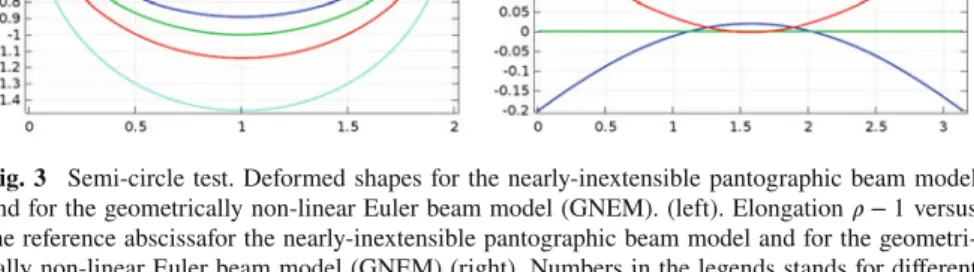
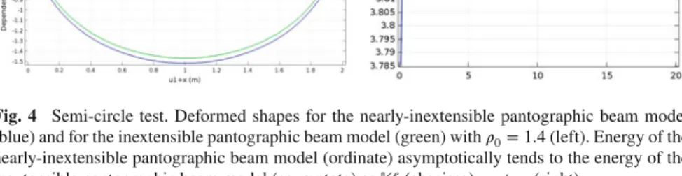
In Fig.3(up) the deformed shapes for the nearly-inextensible pantographic beam model and for the geometrically non-linear Euler beam model (GNEM) are shown for different values of𝜌0 reported in the legend. In Fig.3 (down) the elongation 𝜌 − 1 for the nearly-inextensible pantographic beam model and for the geometrically non-linear Euler beam model (GNEM) is shown for different values of𝜌0reported in the legend. It is remarkable that passing from𝜌0> 1 to 𝜌 < 1 there is a change of concavity in the elongation for the pantographic beam model. In Fig.4(up) the deformed shapes for the nearly-inextensible pantographic beam model (blue) and for the inextensible pantographic beam model (green) with𝜌0 = 1.4 are compared. Of course, the area spanned by the quasi-inextensible pantographic beam includes that
Fig. 3 Semi-circle test. Deformed shapes for the nearly-inextensible pantographic beam model and for the geometrically non-linear Euler beam model (GNEM). (left). Elongation𝜌 − 1 versus the reference abscissafor the nearly-inextensible pantographic beam model and for the geometri-cally non-linear Euler beam model (GNEM) (right). Numbers in the legends stands for different dimensionless values of𝜌0
Fig. 4 Semi-circle test. Deformed shapes for the nearly-inextensible pantographic beam model (blue) and for the inextensible pantographic beam model (green) with𝜌0= 1.4 (left). Energy of the nearly-inextensible pantographic beam model (ordinate) asymptotically tends to the energy of the inextensible pantographic beam model (asymptote) as𝕂e(abscissa)→ +∞ (right)
of the (completely) inextensible one. In Fig.4(down) it is numerically shown that the energy of the nearly-inextensible pantographic beam model (ordinate) asymptot-ically tends to the energy of the inextensible pantographic beam model (asymptote) as𝕂e(abscissa)→ +∞.
4.2 Three-Point Test
We consider for both the quasi-inextensible pantographic beam model and the geo-metrically non-linear Euler beam model the reference domain to be the interval[0, 2]. We enforce the following boundary conditions for both models:
1. 𝜒 (0) = 𝟎; 2. 𝜒 (1) ⋅ 𝐞2= u; 3. 𝜒 (2) = 𝟎; 4. 𝜗 (0) = 0; 5. 𝜗 (2) = 0.
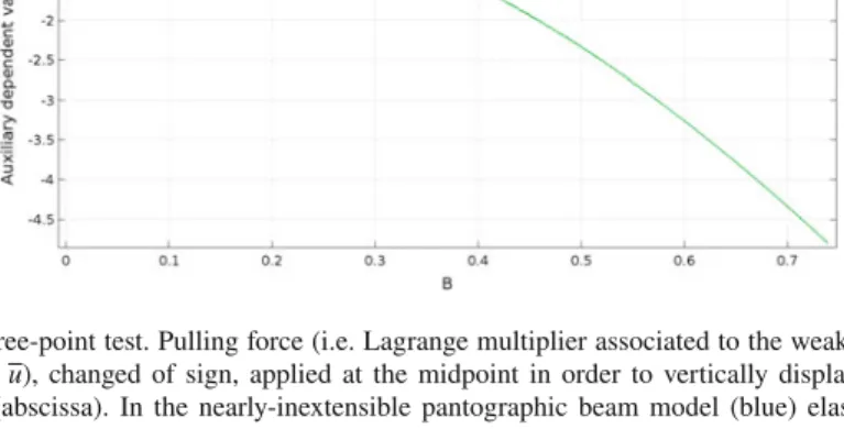
In Fig.5 the deformed shapes for the nearly-inextensible pantographic beam model (red, light blue) and for the geometrically non-linear Euler beam model (blue, green) are shown for different values ofu in the legend. Figure6shows, for different values of the parameteru, the elongation 𝜌 − 1 versus the reference abscissa for the nearly-inextensible pantographic beam model. The parameteru is increasing from bottom to top. We observe that, asu increases, at some point, there is a concavity change in the elongation plot and, increasing further the parameteru, curves start to intersect. This means that, for some points of the beam an increase of the prescribed displacementu implies a decrease in the elongation. Figure7shows the pulling force, i.e. Lagrange multiplier associated to the weak constraint𝜒 (1) ⋅ 𝐞2= u, changed of sign, applied at the midpoint in order to vertically displace it of an amountu. In the nearly-inextensible pantographic beam model (blue) negative stiffness property, also known as elastic softening, is observed, while in the geometrically non-linear Euler beam model (green) elastic softening is not observed. Figure8shows the plot of ̃l1D versus reference abscissa for different values of u in the legend. Analogous plots hold for ̃l2D, ̃l1Sand ̃l2S.
Fig. 5 Three-point test. Deformed shapes for the nearly-inextensible pantographic beam model (red, light blue) and for the geometrically non-linear Euler beam model (blue, green) for different values of u in the legend
Fig. 6 Three-point test. Elongation𝜌 − 1 versus the reference abscissa for the nearly-inextensible pantographic beam model. The parameter u is increasing from bottom to top. We observe that, While increasing u, there is a concavity change at some point. Increasing further the parameter u, curves start to intersect
4.3 Modified Three-Point Test
We consider for both the quasi-inextensible pantographic beam model and the geo-metrically non-linear Euler beam model the reference domain to be the interval[0, 2]. We enforce the three-point test boundary conditions for both models
1. 𝜒 (0) = 𝟎; 2. 𝜒 (1) ⋅ 𝐞2= u; 3. 𝜒 (2) = 𝟎; 4. 𝜗 (0) = 0; 5. 𝜗 (2) = 0
with the additional condition, at the midpoint s = 1, 6. 𝜌 (1) ≃√2.
Fig. 7 Three-point test. Pulling force (i.e. Lagrange multiplier associated to the weak constraint
𝜒 (1) ⋅ 𝐞2= u), changed of sign, applied at the midpoint in order to vertically displace it of an
amount u (abscissa). In the nearly-inextensible pantographic beam model (blue) elastic soften-ing is observed, while in the geometrically non-linear beam model (green) elastic softensoften-ing is not observed
Fig. 8 Three-point test. Plot of ̃l1Dversus reference abscissa for different values of u in the legend. Analogous plots hold for ̃l2D, ̃l1Sand ̃l2S
Fig.9 shows the deformed configuration for the nearly-inextensible pantographic beam model, while in Fig.10the elongation𝜌 − 1 versus the reference abscissa for the nearly-inextensible pantographic beam model is shown.
5
Euler-Lagrange Equations
Let us consider an internal (potential) unit line energy density of the form
W = G2(𝜌)𝜌′2+F2(𝜌)𝜗′2+ H (𝜌) (31) with𝜌 and 𝜗 such that 𝜒′= 𝜌(cos 𝜗𝐞1+ sin 𝜗𝐞2)= 𝜌𝐞 (𝜗), and G, F, H functions fromℝ+⊇ A to ℝ+. We recall that𝜌′= 𝜒′′⋅𝜒′
‖𝜒′‖,𝜗′=
𝜒′′⋅𝜒′ ⟂
Fig. 9 Modified three-point test. Deformed configuration for the nearly-inextensible pantographic beam model
Fig. 10 Modified three-point test. Elongation𝜌 − 1 versus reference abscissa for the nearly-inextensible pantographic beam model
the specialization ⎧ ⎪ ⎨ ⎪ ⎩ G(𝜌) = 0 F(𝜌) = Kb≥ 0 H(𝜌) = K2e(𝜌 − 1)2, Ke≥ 0 (32)
of (31) is considered, we find the geometrically nonlinear Euler model while, when the specialization ⎧ ⎪ ⎪ ⎨ ⎪ ⎪ ⎩ G(𝜌) = 𝕂e𝕂f 𝜌2 (2−𝜌2)[𝜌2(𝕂e−4𝕂f)+8𝕂f], 𝕂e≥ 0, 𝕂f ≥ 0 F(𝜌) = 𝕂e𝕂f (𝜌2−2) 𝜌2(𝕂e−4𝕂f)−2𝕂e, 𝕂e≥ 0, 𝕂f ≥ 0 H(𝜌) = 𝕂2m (𝜌 − 1)2, 𝕂m> 0 (33)
of (31) is considered, we find the nearly-inextensible pantographic beam model. We now consider the functional
(𝜌 (⋅) , 𝜗 (⋅) , 𝜒 (⋅) , Λ (⋅)) = = ∫{W − bext⋅ 𝜒 − 𝜇ext⋅ 𝜗 + Λ ⋅[𝜒′− 𝜌𝐞 (𝜗)]} ds+ −∑ s=0,L Rext(s) ⋅ 𝜒 (s) −∑ s=0,L Mext(s) ⋅ 𝜗 (s) , (34)
where ∫bext⋅ 𝜒 + 𝜇ext⋅ 𝜗 ds +∑
s=0,LRext(s) ⋅ 𝜒 (s) +
∑
s=0,LMext(s) ⋅ 𝜗 (s) is the
work done by external distributed and concentrated forces and couples. The first variation of the functional in (34) is
𝛿 (𝜌 (⋅) , 𝜗 (⋅) , 𝜒 (⋅) , Λ (⋅) , 𝛿𝜌 (⋅) , 𝛿𝜗 (⋅) , 𝛿𝜒 (⋅) , 𝛿Λ (⋅)) = = ∫ { 1 2𝜕G𝜕𝜌 (𝜌) 𝜌′2+ 12𝜕F𝜕𝜌(𝜌) 𝜗′2+ 𝜕H𝜕𝜌 (𝜌) − Λ ⋅ 𝐞 (𝜗) − [ G(𝜌) 𝜌′]′ } 𝛿𝜌 ds + + ∫{−[F(𝜌) 𝜗′]′− 𝜇 − Λ × 𝜒′ } 𝛿𝜗 +(−b − Λ′)⋅ 𝛿𝜒 +[𝜒′− 𝜌𝐞 (𝜗)]⋅ 𝛿Λ ds + +[G(𝜌) 𝜌′𝛿𝜌]L0+{[F(𝜌) 𝜗′− Mext]𝛿𝜗}L0+[(Λ − Rext)⋅ 𝛿𝜒]L0= = ∫ { 1 2𝜕F𝜕𝜌(𝜌) 𝜗′2+ 𝜕H𝜕𝜌 (𝜌) − 12𝜕G𝜕𝜌(𝜌) 𝜌′2− Λ ⋅ 𝐞 (𝜗) − G (𝜌) 𝜌′′ } 𝛿𝜌 ds + + ∫ { −[F(𝜌) 𝜗′]′− 𝜇 − Λ × 𝜒′ } 𝛿𝜗 +(−b − Λ′)⋅ 𝛿𝜒 +[𝜒′− 𝜌𝐞 (𝜗)]⋅ 𝛿Λ ds + +[G(𝜌) 𝜌′𝛿𝜌]L0+{[F(𝜌) 𝜗′− Mext]𝛿𝜗}L0+[(Λ − Rext)⋅ 𝛿𝜒]L0.
By applying the Fundamental Lemma of Calculus of Variations, we find the Euler-Lagrange equations: 1. 1 2 𝜕G 𝜕𝜌 (𝜌) 𝜌′2+ 12 𝜕F 𝜕𝜌 (𝜌) 𝜗′2+ 𝜕H𝜕𝜌 (𝜌) − Λ ⋅ 𝐞 (𝜗) − [ G(𝜌) 𝜌′]′= 0 2. [F(𝜌) 𝜗′]′+ 𝜇 + Λ × 𝜒′= 0 3. b + Λ′= 0 4. 𝜒′− 𝜌𝐞 (𝜗) = 0
and the corresponding boundary conditions:
G(𝜌 (0)) = 0 ∨ 𝜌′(0) = 0 ∨ Dirichlet Conditions on 𝜌 in s = 0 G(𝜌 (L)) = 0 ∨ 𝜌′(L) = 0 ∨ Dirichlet Conditions on 𝜌 in s = L
F(𝜌 (0)) 𝜗′(0) − Mext(0) = 0 ∨ Dirichlet Conditions on 𝜗 in s = 0 F(𝜌 (L)) 𝜗′(L) − Mext(L) = 0 ∨ Dirichlet Conditions on 𝜗 in s = L
Λ (0) − Rext(0) = 0 ∨ Dirichlet Conditions on 𝜒 in s = 0
Λ (L) − Rext(L) = 0 ∨ Dirichlet Conditions on 𝜒 in s = L.
We now analyze the two specializations (32) and (33) of (31). Let us first analyze (32). The Euler-Lagrange equations reduce to
1. Ke(𝜌 − 1) − Λ ⋅ 𝐞 (𝜗) = 0
2. [Kb𝜗′]′+ 𝜇 + Λ × 𝜒′= 0
3. b + Λ′= 0
4. 𝜒′− 𝜌𝐞 (𝜗) = 0, (35)
complemented with the following boundary conditions
Kb𝜗′(0) − Mext(0) = 0 ∨ Dirichlet Conditions on 𝜗 in s = 0 Kb𝜗′(L) − Mext(L) = 0 ∨ Dirichlet Conditions on 𝜗 in s = L
Λ (0) − Rext(0) = 0 ∨ Dirichlet Conditions on 𝜒 in s = 0
Λ (L) − Rext(L) = 0 ∨ Dirichlet Conditions on 𝜒 in s = L. (36)
We notice that (35)1is an algebraic equation in𝜌, and it gives: 𝜌 = 1 +Λ ⋅ 𝐞 (𝜗)
The direct integration of Eq. (35)3gives:
Λ = ∫0sb ds + Rext(0) , (38)
while, plugging (38) in (37) yields 𝜌 = 1 + [ ∫s 0 b ds + Rext(0) ] ⋅ 𝐞 (𝜗) Ke , (39)
and plugging (39) and (38) in (35)2yields [ Kb𝜗′]′+ 𝜇 + Λ × ( 1 +Λ ⋅ 𝐞 (𝜗) Ke ) 𝐞 (𝜗) = 0,
which is a 2nd order O.D.E. in the unknown𝜗. This O.D.E. is complemented with boundary conditions (36)1,2. Finally, one recovers𝜒 by integrating (35)4and by using the Dirichlet boundary conditions on𝜒. Let us turn to the study of the specialization (33) of the unit line potential energy density in Eq. (31). By explicitly computing the partial derivatives of the functions F, G, H with respect to 𝜌, we get the following Euler-Lagrange equations for the nearly-inextensible pantographic beam model:
1. 𝕂e𝕂f [ 16𝕂f𝜌 + (𝕂e− 4𝕂f)𝜌5] (𝜌2− 2)2[(𝕂e− 4𝕂f)𝜌2+ 8𝕂f]2𝜌 ′2− 16𝕂e ( 𝕂f)2𝜌 [ (𝕂e− 4𝕂f)𝜌2− 2𝕂e)]2𝜗 ′2+ 𝕂m(𝜌 − 1) − Λ ⋅ 𝐞(𝜗) + − [ 𝕂e𝕂f( 𝜌2𝜌′ 2 − 𝜌2) [𝜌2(𝕂e− 4𝕂f)+ 8𝕂f] ]′ = 0 2. [ 𝕂e𝕂f ( 𝜌2− 2) 𝜌2(𝕂e− 4𝕂f)− 2𝕂e𝜗 ′] ′ + 𝜇 + Λ × 𝜒′= 0 3. b + Λ′= 0 4. 𝜒′− 𝜌𝐞 (𝜗) = 0,
complemented with the following boundary conditions:
𝜌′(0) = 0 ∨ Dirichlet Conditions on 𝜌 in s = 0 𝜌′(L) = 0 ∨ Dirichlet Conditions on 𝜌 in s = L 𝕂e𝕂f ( 𝜌2(0) − 2) 𝜌2(0) (𝕂e− 4𝕂f) − 2𝕂e𝜗
′(0) − Mext(0) = 0 ∨ Dirichlet Conditions on 𝜗 in s = 0
𝕂e𝕂f
(
𝜌2(L) − 2)
𝜌2(L) (𝕂e− 4𝕂f) − 2𝕂e𝜗
′(L) − Mext(L) = 0 ∨ Dirichlet Conditions on 𝜗 in s = L
Λ (0) − Rext(0) = 0 ∨ Dirichlet Conditions on 𝜒 in s = 0
For the (completely) inextensible pantographic beam model, from Eq. (29) we have that:
G(𝜌) = 2 − 𝜌2𝕂f2 F(𝜌) = 2𝕂f
H(𝜌) = 𝕂m(𝜌 − 1)2.
Therefore, Euler-Lagrange equations for the inextensible pantographic beam model recast as 1. 2𝜌𝕂f (2 − 𝜌2)2𝜌′2+ 2𝕂m(𝜌 − 1) − Λ ⋅ 𝐞(𝜗) − [ 2𝕂f 2 − 𝜌2𝜌′ ] = 0′ 2. 𝜇 + Λ × 𝜒′= 0 3. b + Λ′= 0 4. 𝜒′− 𝜌𝐞 (𝜗) = 0,
complemented with the following boundary conditions: 𝜌′(0) = 0 ∨ Dirichlet Conditions on 𝜌 in s = 0
𝜌′(L) = 0 ∨ Dirichlet Conditions on 𝜌 in s = L
2𝕂f𝜗′(0) − Mext(0) = 0 ∨ Dirichlet Conditions on 𝜗 in s = 0
2𝕂f𝜗′(L) − Mext(L) = 0 ∨ Dirichlet Conditions on 𝜗 in s = L
Λ (0) − Rext(0) = 0 ∨ Dirichlet Conditions on 𝜒 in s = 0
Λ (L) − Rext(L) = 0 ∨ Dirichlet Conditions on 𝜒 in s = L.
We believe that the use of the techniques employed in [74], which have been exploited to analytically determine remarkable properties of the extensible Euler beam model in finite deformation regime, can be fruitfully applied to the examined pantographic beam model. Also the numerical exploitation of the Euler-Lagrange equations through, e.g., a shooting method, could be useful to explore the set of solutions. This might be of help in shedding light on the mathematical properties of the quasi-inextensible and inextensible pantographic beam models.
6
Conclusions
In this work, we have modeled and analyzed a pantographic microstructure giving rise, after a homogenization procedure, to a1D continuum model for a beam which
exhibits many interesting non-standard features. We have provided a characterization of the kinematics of the proposed discrete Hencky-type spring model which resem-bles the geometrical arrangement of a pantographic strip. Once the kinematics of the micro-model has been discussed, we have given a mechanical characterization of the micro-system, by specifying the general form of the deformation energy. Sub-sequently, we postulated an asymptotic expansion for one of the microscopic descrip-tors, i.e. the elongation of the oblique springs. Besides, by choosing the value of the first-order term of this expansion, we considered the so-called quasi-inextensibility case, which corresponds to the quasi-inextensibility of the oblique springs. Succes-sively, following the Piola’s ansatz, we introduced the so-called kinematical maps, i.e. some fields in the macroscopic model that uniquely determine the microscopic kinematical descriptors. By means of these kinematical maps, namely the placement function𝜒 and the elongation of the oblique springs ̃l𝛼𝛽, we have written the micro-model energy for the quasi-inextensibility case in terms of macroscopic descriptors. The resulting micro-model energy contains already a contribution from the second gradient of𝜒(s) and it provides an upper bound ||𝜒′|| <√2, even if no kinematic restrictions directly affect||𝜒′||. Successively, we have considered the case of (com-pletely) inextensible oblique springs by means of two equivalent procedures. We also verified that, as it is obvious, requiring the kinematic descriptor ̃l𝛼𝛽, standing for the elongation of the oblique springs, to vanish implies that the quasi-inextensible pantographic beam model specializes to the (completely) inextensible pantographic beam model. In order to give a better insight into the peculiar properties of this problem, we also derived “ab imis fundamentis” the micro-model energy of the inextensible pantographic beam model, whose kinematics is characterized by the positions pionly, as a function of the macroscopic kinematical descriptor𝜒
eval-uated in si’s. Following a procedure analogue to the quasi-inextensibility case, we
defined the micro-model energy for the inextensibility case and, once the kinemati-cal maps was introduced by means of the Piola’s ansatz, we have written it in terms of these macroscopic descriptors. Then, we have imposed the so-called internal con-nection constraint, which ensures that, in the deformed configuration, the upper-left spring of the i-th cell is hinge-joint with the upper-right spring of the (i − 1)-th cell, and the lower-left spring of the i-th cell is hinge-joint with lower-right spring of the (i − 1)-th cell. After that, we have performed a heuristic homogenization procedure in order to derive a1D continuum model, also referred to as the macro-model and characterized by its deformation energy, associated to the aforementioned micro-structure in the quasi-inextensibility and inextensibility cases. The preliminary step to perform the homogenization procedure has been to define scale-invariant quan-tities, whose role is to keep track of the asymptotic behaviour of the stiffnesses of the micro-model springs. We first performed the homogenization procedure for the quasi-inextensibility case by computing the limit 𝜀 → 0 in the expression of the micro-model energy written in terms of macroscopic kinematical descriptors. The resulting continuum-limit macro-model energy describes a1D pantographic beam under the hypothesis of quasi-inextensible oblique micro-springs. The macroscopic beam, when𝕂m= 0, ̃l𝛼𝛽 = 0, and 𝜒(s) = Cse
a key feature of the micro-model energy which was preserved by the homogeniza-tion procedure that we have carried out. Moreover, we observed that not only this homogenized model can be classified as a second gradient theory, but we noticed that the full second gradient𝜒′′of𝜒 contributes to the strain energy. Indeed, beyond the usual term(𝜒⟂′ ⋅ 𝜒′′) related to the Lagrangian curvature, also the term (𝜒′⋅ 𝜒′′), deriving from the presence of the oblique springs, appears. Finally, we remarked that, in the limit||𝜒′|| →√2, the model exhibits a so-called phase transition, i.e. it locally degenerates into the model of an uniformly extensible cable, notwithstanding that√2 is an upper bound for 𝜌. Subsequently, we have performed the homogeniza-tion procedure also for the (complete) inextensibility case. The homogenizahomogeniza-tion pro-cedure has followed the same lines of the quasi-inextensibility case and it yields a continuum-limit macro-model energy consistent with the quasi-inextensibility case. An interesting connection with the existing literature on1D continuum homogenized models for microstructured media, and in particular for pantographic ones, has been traced by considering the linearization of the pantographic beam energy in the (com-plete) inextensibility case. Furthermore, it has to be remarked that, of course, what has been presented in this paper is not the only possible homogenization technique. Indeed, many other procedures, like coarse-graining, hydrodynamical limits [76–79] for many-particle systems, and computational homogenization [80–82], are being employed in literature, and they deserve to be better understood. The numerical solu-tion of the homogenised continuum model has been addressed by means of the finite element method in three exemplary cases, trying to highlight the main differences with the classical finite deformation Euler beam model. In particular, in order to better highlight some non-standard features of the nearly-inextensible pantographic beam model, we have considered as vanishing the standard quadratic additive elonga-tion/shortening contribution to the deformation energy. These benchmark tests were exploited in order to illustrate some peculiar features of the pantographic beam model and the convergence of the quasi-inextensible pantographic beam model to the com-pletely inextensible one. In particular, we have performed for the nearly-inextensible pantographic beam model and for the geometrically non-linear Euler model what has been referred to as the semi-circle test, the point test and the modified three-point test. The weak form deriving from the stationarity of the energy functional has been projected on the basis of Hermite cubic interpolants. Further improvements of this approach could include the use of isogeometric analysis, which has found wide application for beam elements [83–91]. Indeed, spline functions employed in that approach allow to ensure higher continuity between elements and other many desir-able properties. Finally, through a standard variational procedure, we have provided the explicit form of the Euler-Lagrange equations and of the corresponding boundary conditions for a general potential energy density functional which includes as par-ticular cases the quasi-inextensible pantographic beam model and the Euler beam model. Moreover, we have given the explicit form of the Euler-Lagrange equations and of the boundary conditions for the quasi-inextensible and completely inextensi-ble pantographic beam model. It is conceivainextensi-ble that pantographic beams can be used as building blocks for more complex double scale materials.
References
1. Euler, L., Carathéodory, C.: Methodus Inveniendi Lineas Curvas Maximi Minimive Proprietate Gaudentes Sive Solutio Problematis Isoperimetrici Latissimo Sensu Accepti, vol. 1. Springer Science & Business Media (1952)
2. Antman, S.S.: Nonlinear Problems of Elasticity. Mathematical Sciences, vol. 107. Springer, Berlin, New York (1995)
3. Placidi, L., Barchiesi, E., Battista, A.: An inverse method to get further analytical solutions for a class of metamaterials aimed to validate numerical integrations. In: Mathematical Modelling in Solid Mechanics, pp. 193–210. Springer (2017)
4. Murat, F., Sili, A.: Comportement asymptotique des solutions du système de l’élasticité linéarisée anisotrope hétérogène dans des cylindres minces. Comptes Rendus de l’Académie des Sciences-Series I-Mathematics 328(2), 179–184 (1999)
5. Mora, M.G., Müller, S.: A nonlinear model for inextensible rods as a low energy𝛾-limit of three-dimensional nonlinear elasticity. Annales de l’IHP Analyse non linéaire 21, 271–293 (2004)
6. Jamal, R., Sanchez-Palencia, E.: Théorie asymptotique des tiges courbes anisotropes. Comptes rendus de l’Académie des sciences. Série 1, Mathématique 322(11), 1099–1106 (1996) 7. Pideri, C., Seppecher, P.: Asymptotics of a non-planar rod in non-linear elasticity. Asymptot.
Anal. 48(1, 2), 33–54 (2006)
8. Allaire, G.: Homogenization and two-scale convergence. SIAM J. Math. Anal. 23(6), 1482– 1518 (1992)
9. Bensoussan, A., Lions, J.-L., Papanicolaou, G.: Asymptotic Analysis for Periodic Structures, vol. 5. North-Holland Publishing Company Amsterdam (1978)
10. Alibert, J.-J., Seppecher, P., dell’Isola, F.: Truss modular beams with deformation energy depending on higher displacement gradients. Math. Mech. Solids 8(1), 51–73 (2003) 11. Carcaterra, A., dell’Isola, F., Esposito, R., Pulvirenti, M.: Macroscopic description of
micro-scopically strongly inhomogeneous systems: a mathematical basis for the synthesis of higher gradients metamaterials. Arch. Ration. Mech. Anal. 218(3), 1239–1262 (2015)
12. Abali, B.E., Müller, W.H., dell’Isola, F.: Theory and computation of higher gradient elasticity theories based on action principles. Arch. Appl. Mech. 1–16 (2017)
13. Pietraszkiewicz, W., Eremeyev, V.: On natural strain measures of the non-linear micropolar continuum. Int. J. Solids Struct. 46(3), 774–787 (2009)
14. Altenbach, H., Eremeyev, V.: On the linear theory of micropolar plates. ZAMM-Journal of Applied Mathematics and Mechanics/Zeitschrift für Angewandte Mathematik und Mechanik
89(4), 242–256 (2009)
15. dell’Isola, F., Della Corte, A., Giorgio, I.: Higher-gradient continua: the legacy of piola, mindlin, sedov and toupin and some future research perspectives. Math. Mech. Solids (2016). https://doi.org/10.1177/1081286515616034
16. dell Isola, F., Seppecher, P., Della Corte, A.: The postulations á la d alembert and á la cauchy for higher gradient continuum theories are equivalent: a review of existing results. In: Proceedings of the Royal Society A, vol. 471, p. 20150415. The Royal Society (2015)
17. dell’Isola, F., Giorgio, I., Andreaus, U.: Elastic pantographic 2D lattices: a numerical analysis on static response and wave propagation. Proc. Est. Acad. Sci. 64, 219–225 (2015)
18. Reiher, J.C., Giorgio, I., Bertram, A.: Finite-element analysis of polyhedra under point and line forces in second-strain gradient elasticity. J. Eng. Mech. 143(2), 04016112 (2016)
19. Boutin, C., Giorgio, I., Placidi, L., et al.: Linear pantographic sheets: asymptotic micro-macro models identification. Math. Mech. Complex Syst. 5(2), 127–162 (2017)
20. dell’Isola, F., Cuomo, M., Greco, L., Della Corte, A.: Bias extension test for pantographic sheets: numerical simulations based on second gradient shear energies. J. Eng. Math. 1–31 (2016)
21. Seppecher, P., Alibert, J.-J., dell’Isola, F.: Linear elastic trusses leading to continua with exotic mechanical interactions. In: Journal of Physics: Conference Series, vol. 319, p. 012018. IOP Publishing (2011)