HAL Id: cea-02430130
https://hal-cea.archives-ouvertes.fr/cea-02430130
Submitted on 7 Jan 2020
HAL is a multi-disciplinary open access
archive for the deposit and dissemination of
sci-entific research documents, whether they are
pub-lished or not. The documents may come from
teaching and research institutions in France or
abroad, or from public or private research centers.
L’archive ouverte pluridisciplinaire HAL, est
destinée au dépôt et à la diffusion de documents
scientifiques de niveau recherche, publiés ou non,
émanant des établissements d’enseignement et de
recherche français ou étrangers, des laboratoires
publics ou privés.
measurements of the fluctuating temperature in the
solid wall
Olivier Braillard, Richard Howard, Kristian Angele, Afaque Shams, Nicolas
Edh
To cite this version:
Olivier Braillard, Richard Howard, Kristian Angele, Afaque Shams, Nicolas Edh. Thermal mixing
in a T-junction: Novel CFD-grade measurements of the fluctuating temperature in the solid wall.
Nuclear Engineering and Design, Elsevier, 2018, 330, pp.377-390. �10.1016/j.nucengdes.2018.02.020�.
�cea-02430130�
Commissariat à l’Energie Atomique et aux Energies Alternatives, France
bÉlectricité de France R&D, France cVattenfall AB, Sweden
dNuclear Research and Consultancy Group, The Netherlands eForsmarks Kraftgrupp AB, Sweden
A R T I C L E I N F O
Keywords: Thermal fatigue T-junction Experiments Novel senor Sharp corner Round cornerA B S T R A C T
This article reports new experiments performed with the purpose of generating novel data of thefluctuating temperature inside the solid in the mixing region between hot and cold water in a T-junction. This data has been measured using a novel sensor (coefh) developed at the Commissariat à l’Energie Atomique et aux Energies Alternatives (CEA) in Cadarache, France. These experiments are performed within the framework of the MOTHER project. The main objective of the MOTHER project is to validate various CFD approaches (such as LES, Hybrid i.e. RANS/LES and RANS) for transient heat transfer in a T-junction configuration including the pipe wall. Hence, the performed experiments have focused on accurately measuring and documenting the boundary conditions to be able to have a well-defined database for CFD validation. The tests are performed for two different Reynolds numbers 40000 and 60000 and for two different T-junction geometries; a sharp corner and a round corner.
1. Introduction
Thermal fatigue is a degradation mechanism which occurs in a wide range of industrial applications. One such application is the primary piping system of a nuclear power plant, where the mixing offlows with different temperature can lead to thermal fatigue. The consequences of thermal fatigue can be serious and can cause sufficient structural da-mage for a power plant to require a complete shut-down. Therefore, it is highly relevant in the context of aging and the life time management of a nuclear power plant. In the last decade, several efforts have been made for the assessment of thermal fatigue (Braillard et al., 2006; Chapuliot et al., 2005; Coste et al., 2008; Fontes et al., 2009; Kamide et al., 2009; Smith et al., 2013). The generic configuration that is mostly considered is the T-junction, where the mixing of two separate hot and cold streams occur immediately downstream of the T-junction. This transient turbulent mixing results in high temperaturefluctuations next to and inside the pipe walls. Thefirst step is, however, to be able to predict the temperaturefluctuations in the fluid close to the wall. In this regard, an extensive amount of research work has been performed in relation to the application of CFD for the assessment of thermal fatigue in the T-junction (Gillis et al., 2013; Howard and Pasutto, 2009; Jayaraju et al., 2010; Kuhn et al., 2010; Nakamura et al., 2009; Westin
et al., 2008).
In the recent past, an attempt was made to evaluate the accuracy in the CFD predictions such thermalfluctuations in the form of the OECD CFD Benchmark for the Vattenfall T-junction configuration (Smith et al., 2013). The considered configuration was based on adiabatic walls. As an outcome of the benchmarking exercise, one of the re-commendations was the need for more insights into the heat transfer phenomenon from thefluid flow to the wall. This recommendation was the main motivation behind the MOTHER project, with the purpose of generating novel data of thefluctuating temperature in the solid wall for the validation of CFD calculations.
The main objective of theMOTHER project (Modelling T-junction HEat TransfeR) is to validate various CFD approaches (such as LES, Hybrid (RANS/LES) and RANS) for transient heat transfer in a T-junc-tion configuraT-junc-tion including the wall with new experimental data. These CFD calculations have to take into account the effect of the wall and the heat transfer. The mean andfluctuating fields of the velocity and the temperature (fluid and wall) are also evaluated. The effects of the mixing tee geometry (a round and a sharp corner) as well as Reynolds numbers (Re) are investigated at Re = 40000 and Re = 60000. The FATHERINO facility at CEA in Cadarache is used as the test facility. This facility is specifically designed to study the
https://doi.org/10.1016/j.nucengdes.2018.02.020
Received 31 October 2017; Received in revised form 13 February 2018; Accepted 14 February 2018
⁎Corresponding author.
E-mail address:shams@nrg.eu(A. Shams).
Available online 20 February 2018
thermal loads for mixing in T-junction geometries. The instrumentation includes Laser Doppler Velocimetry (LDV) and thermocouples for the measurement of temperature. The advanced“coefh” sensor is used for the latter. The description of the FATHERINO test facility is given in Section 2. Details of the measurement techniques and the boundary conditions are given in Section3. In Section4, the results in the mixing region are reported. This is followed by the conclusions in Section5. 2. The FATHERINO experimental setup
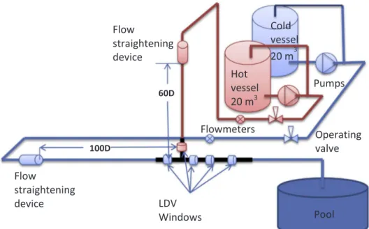
The experimental setup is composed of an equal T-junction (54 mm × 54 mm in diameter D) connected to two straight upstream pipes, i.e. a direct and a perpendicular branch, as shown inFig. 1. The straight direct branch carries the cold water and is 100 D long, whereas, the straight perpendicular branch is 60 D long and carries the hot water. These pipes are composed of successive sections of PVC (polyvinyl chloride material) and stainless steel close to the T-junction and the whole system is connected by theflanges (Fig. 1).
Two independent pumps are installed to supply theflows to the T-junction. In addition, two operating valves (controlled by the flow meters) are used to keep theflow rates constant during the decreasing water level in the respective vessels. The capacity of each vessel is 20 m3, which is sufficient in order to perform a test during several hours
with the currentflow rates.
In order to reduce the effects of the pipe bends, two flow straigh-tening devices are installed before the straight pipes. These devices consist of cylinders with several long drilled parallel holes followed by threefine grids in order to generate evenly distributed velocity profiles with homogeneous turbulence.
2.1. The mock-ups
2.1.1. The stainless steel 304L mock-ups
Two internal geometries are investigated, one sharp corner and one round corner, as shown inFig. 2. The common dimensions for the 304L mock-ups are a nominal internal diameter of 54 mm with a thickness of 9.53 mm. The diameter of the 304L mock-ups has been controlled and it has been found to be between 53.80 mm <∅ < 53.97 mm. The in-ternal radius, R, of the roundness of the intersection between the two pipes is less than 1 mm for the sharp corner (i.e. can be assumed to be perfectly sharp in CFD) and R = 18 mm for the round corner.
The surface roughness has been measured (of the order of 1–10 μm) and it can be concluded that it is safe to assume hydraulically smooth pipes in the CFD considering the values of the skin friction in the tests. The stainless steel is used for the mock-ups is 304L with the following
Fig. 1. The FATHERINO facility– overall view with the long straight pipes.
properties:
•
Specific heat capacity: cp= 460 J/kg.K•
Thermal conductivity:λ = 16 W/m.K•
Density:ρ = 7821 kg/m3•
Diffusivity: α = 0.445 105m2/s
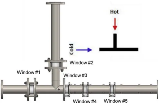
The overall view of the mock-up is shown Fig. 3 with the LDV windows. Two are located at the inlets and three in the mixing zone. To change the geometry between the round corner and the sharp corner, only the T-junction part is replaced.
The parts of the mock-ups are assembled by flanges. The LDV windows are inserted between the 304L pipes. The windows are nested with a centering counterbore. Two O-ring gaskets installed on the edges of each LDV window and assure the sealing and allow keeping an in-ternal surface within a minimize gap of 0.3 mm. The rotate part (number 3) is designed on the same principle (Fig. 4).
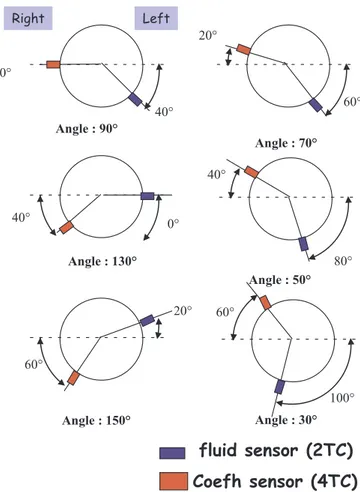
Each measurement section is equipped with two caps, one for the coefh-sensor and one for thefluid sensor. By rotating the pipe, various angles can be measured from 30° to 150° in steps of 20°. The un-certainty in the positioning of the angle is of the order of 1°. Some intermediate angles have been performed in the sensitive part of the
mixing region (80° and 100°), seeFig. 5. A right handed coordinate system is used as follows. The origin is where the axis of the main and branch pipe intersect. The x-axis is defined as positive in the flow di-rection of the main pipe. The z-axis is defined as positive such that gravity is in the negative z-direction.
2.1.2. The brass mock-up
The infrared measurements are performed with the brass mock-ups (round and sharp corner). Their internal geometries are identical to the 304L mock-ups, except the thickness reduced to 1 mm for providing the bandwidth of the thermal radiation. This mock-up is also called“the skin of thefluid” to remember that this thin structure like a skin is used as a frontier of theflow.
The brass mock-ups are used for temperature mapping in the mixing zone. The mock-ups supply local information to improve the knowledge on the effect of the corner. The brass mock-up favours a large diffusivity (factor 7.5 better than 304L).
= Biot number h e
λ .
(h: heat transfer coefficient; e: thickness; λ: wall conductivity). As the thickness is low (1 mm), the Biot number is low (less than
Fig. 3. 304L mock-up with 5 windows for the LDV measurements.
0.05), that means the temperature fluctuating sampled between the inner and outer surface is weakly reduced. Nevertheless, the diffusivity in the perpendicular direction is also great and this effect in the per-pendicular direction is not attenuated and reduces the sharpness of the infrared frames. The infrared camera is located in the mixing zone (closed and far from the tee junction to cover a large area of interest.
The common dimensions for the brass mock-up are a nominal in-ternal diameter: 53 mm with a thickness: 1 mm. For the brass mock-up, only the central part (i.e. the T-junction) is removed to switch between the configurations. The inlets straight pipes (vertical and horizontal) are connected to the junction part without welding as well as the outlet pipes. The overall dimensions of the brass mock-ups are similar to the 304L mock-ups. The main properties of the brass mock-ups are as fol-lows:
•
Heat mass: 385 J/kg.K•
Thermal conductivity: 111 W/m.K•
Density: 8522 kg/m3•
Diffusivity: 3.383 10−5m2/s3. Measurement techniques and boundary conditions 3.1. Massflow rates
Theflowrates are measured by two conductivity flowmeters with an uncertainty of about 0.5% of full range (0.15 m3/h). The devices have
been calibrated against a Coriolisflowmeter by an external company qualified for the task. The cold and the hot flowrates are equal. Two Reynolds numbers were tested. The respectiveflowrate and bulk velo-cities are 2.95 m3/h giving an inlet bulk velocity of 0.36 m/s and
4.35 m3/h giving a bulk velocity of 0.53 m/s. Note that all velocities are
normalized with the bulk velocities in the mixing pipe, which is twice the mentioned velocities (more precisely 0.712 m/s and 1.053 m/s, respectively).
3.2. Fluid temperature at the hot and the cold inlets
Two thermocouples measure the temperature at the inlets of the T-junction (insulated K-type∅ 0.5 mm). The position in the fluid is fixed 3 mm from the wall. The uncertainty in such are of the order of 0.1–0.5 °C. The thermocouples are located at 9.9 D before the T-junc-tion for the direct (cold) line and 14.5 D for the perpendicular (hot) line, respectively. The cold and the hot nominal temperatures are 15 °C and 30 °C, respectively. During many of the tests, the temperatures were slightly over the specified nominal values (approximately 1–2 °C), which induces a slight increase in the Reynolds numbers. However, all results are normalized usingΔT = Thot− Tcoldand are quite insensitive
to small variations in the absolute values of the temperatures from day to day.
3.3. Velocity profiles at the hot and the cold inlets
Conventional LDV measurements are used for the velocity and turbulence measurements. In the mixing region, three windowsfilled with water are implemented at the axial distances 1.86 D, 4.95 D, and 9.46 D for LDV measurements. The Plexiglas windows are separated by stainless steel sections.
The mock-ups have been equipped withfive windows in Plexiglas (PMMA), two are located before the T-junction (at x =−4 D) for measurements of the inlet boundary conditions and the others in the mixing area at three different distance downstream from the T-junction. The Plexiglas windows arefilled with water for the laser beams to not be affected by the curved surface of the pipe geometry.
The typical duration for performing a LDV crossing is 20 min at 0.7 m/s (Re = 40000 and 35 s by point) and 15 min at 1.05 m/s (Re = 60000 and 25 s by point). The number of valid data is collected. The criterion is reached when the sampling time or the number of valid data. When 100,000 valid points are recorded, the laser sensor moves automatically to the following location even if the sampling time is not reached. Basically, 100,000 data by point is rarely reached and the sampling time is often reached (35 s or 25 s) before the 100,000 valid data. For the mixing area, the valid data by point for the channel 1 and channel 2 is taken as independent (non-coincidence option selected).
For the velocity profiles at the inlets, only one velocity component in the main direction of theflow was measured (however in two di-rections).
•
Window # 1– horizontal line : U profile versus y-axis and z-axis•
Window # 2– vertical line : W profile versus y-axis and x-axis= = ∗ ∗ U R U R U U R U R U ( ) ( ) ( ) ( ) Bulk RMS RMS Bulk
The velocity profiles corresponding to both Reynolds number are shown inFigs. 6 and 7. It can be concluded that the velocity profiles for the sharp corner and round corner at Re 40000 are very similar, see Fig. 6. In summary, a fully developed turbulent velocity profile can be assumed as a boundary condition (BC) for the CFD calculations (Fig. 8). 3.4. Thermal measurements using the novel coefh-sensor
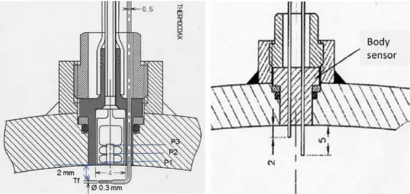
The instrumentation is composed of two advanced temperature sensors in order to get the temperature measurements in the wall and in thefluid. The fluid sensors BF (304L) are composed of two thermo-couples (K-type) ∅ 0.5 mm (time constant = 30 ms) at the distances 2 mm and 5 mm from the wall, seeFig. 9.
The coefh-sensors are made of stainless steel 304L just like the T-junction mock-ups. The three miniature K-type thermocouples (∅
Fig. 5. Angles in the azimuthal direction for the thermal instrumentation. Right and left sides are referenced by the views towards downstream.
25 µm) are located at three distances from the wall (0.4 mm, 1.4 mm and 2.5 mm). One thermocouple K type (∅ 0.3 mm) is located inside thefluid at a distance 2 mm from the wall (Fig. 9). The time constant of the miniature K-type thermocouple is 30 µs and 10 ms for the K type thermocouple in thefluid. The accuracy of the coefh sensor depends of several factor but for the dynamic response, the most important is the perfect knowledge of the distance from the wall of the 3 miniature thermocouples. During the manufacturing, the binocular is used to make measurements with accuracy.
The instrumentation is composed offive coefh-sensors located on the right side of the test section and fourfluid sensors at the same axial distances from the T-junction but on the left side of the pipe. The two rows of caps are welded at 110°, which corresponds to the symmetrical azimuthal angle for the coefh and thefluid sensors (BF), seeFig. 10. To vary and select the different azimuthal angles specified inFig. 5during the measurements, the mixing pipe can be rotated around its x-axis without stopping the test rig.
3.5. Sensors implementation in the mixing zone
The sensors implemented in the mixing zone cover an area from 2.62 D to 8 D (Table 1). The coefh sensor located at 0.5 D (in the T-junction) is used to verify that the temperatures are similar for the three configurations.
4. Results in the mixing region 4.1. Velocity measurements
Figs. 11–13display the velocity profiles and their RMS’s along the y-axis. It can be observed that in the mixing zone closest to the T-junction, at 1.86 D, the difference in the velocity profiles is large between the sharp and the round corner. The U(y)-profile has a large wake with locally lower velocity for the sharp corner contrary to the round corner configuration. The separation zone just behind the vertical line (1.86 D) on the both sides of the x axis is not located at the same position if one compares the U(z)-plots inFigs. 14–16. The Reynolds number does not have a large effect on the velocity profiles for the sharp corner
Fig. 6. Velocity profiles at the boundary conditions – Round corner (left) and Sharp corner (right) at Re = 40000 (U bulk = 0.36 m/s).
Fig. 7. Velocity profiles at the boundary conditions – Sharp corner at Re = 60000 (U bulk = 0.53 m/s).
Fig. 8. Inflow velocity boundary conditions by the (Blue line) Reynolds law model (Red line) LDV measurements. (For interpretation of the references to colour in thisfigure legend, the reader is referred to the web version of this article.)
configuration at any position. The relaxation downstream towards a more uniform velocity profile seem to be faster for the round corner configuration. = = ∗ ∗ U R U R U U R U R U ( ) ( ) ( ) ( ) Bulk RMS RMS Bulk
4.2. RMS offluid and solid temperature
The thermalfield is non-dimensionalized as follows:
= − − ∗ T T Tf Tf Tf Cold Hot Cold (1) = − ∗ T T Tf Tf RMS RMS Hot Cold (2)
For all the thermal tests, the parameters selected for the data ac-quisition are:
•
Acquisition duration: 10 min•
Sampling frequency: 80 HzThe PSD outputs from the temperature measurements in the mixing area are computed upon the following parameters:
•
Block size: 1024 pts•
Weighting window: Hanning•
Frequency resolution: 0.078 Hz•
Frequency bandwidth: 40 Hz•
Number of averaged PSD: 45•
Overlap block: 50%It is worthwhile to mention that the Twis the deduced value at the
inner wall surface temperature by the inverse conduction method. In the range of interest for the CFD-simulations, the RMS temperatures in thefluid and in the solid were computed for the three configurations as a function of the azimuthal angle at four distances (2.62 D, 4.18 D, 5.8 D, and 8 D) from the T-junction (seeFigs. 17–19). In thefluid, the difference between the configurations is small, the maximum values are more centered around 60° for the round corner case and 90° for the sharp corner case. The main difference is the temperature in the solid, which is largely attenuated for the round corner compared to the sharp corner. This could be interpreted as a higher heat transfer from thefluid to the wall in the sharp corner case. The maximumfluctuation in the
Fig. 9. Left: the“coefh” sensor with its three internal thermocouples, P1, P2 and P3. The fluid thermocouple is denoted Tf. Right: The fluid sensor with two thermocouples, the external body is identical to the coefh sensor.
Fig. 10. Implementation of the rows of sensor caps in the T-junction mixing area.
Table 1
Thermal instrumentation in the mixing zone– location of the LDV measurements. Distance from the vertical axis of the perpendicular line (D = 54 mm)
Distance from the vertical axis of the perpendicular line (mm)
Coefh sensor right side
Fluid sensor left side
S0 - Tee #1 & 1′ 0.5 D 27 Coefh03
Window #3 1.86 D 100 LDV– y axis and x axis
S1′ – Mixing section 2.62 D 141.5 Coefh05 BF02
S3– Mixing section 4.18 D 225.6 Coefh07 BF03
Window #4 4.95 D 268 LDV– y axis and x axis
S5– Mixing section 5.8 D 313.3 Coefh20 BF04
S7– Mixing section 8 D 432 Coefh21 BF05
round corner case is obtained at 4.18 D and not at 2.62 D as in the sharp corner case. The increase of the Reynolds number for the sharp corner case enhances the heat transfer as the RMS temperature in the solid increases from 0.023 to 0.033, while thefluctuation in the fluid remains practically the same (Figs. 18 and 19).
4.3. Fluid and solid temperature power spectral density
The power spectral density (PSD) has been computed from the coefh-sensor data. The PSD in Fig. 20 shows five curves, the three measurements in the solid (P1, P2, P3) and one in the fluid (Tf). In addition, the wall temperature (Tw-inv) is computed by solving the inverse heat conduction problem upon a 1D assumption. The time histories from the thermocouples[ ( )]Y t i=1,2,3 are collected and a se-quential inverse conduction algorithm is used to assess thefluctuating heatflux q t() at the wall-fluid limit at =x 0. The method is based on the concepts of “future time-step” and “function specification” (Equation (3)). It means that the heatflux at the time q t( )k is computed from the
temperature measurements later than tk.
Equation 3: Inverse conduction algorithm.
̂
∑ ∑
= + − + = = q t(k ) q t( )k [ ( )Y t T t( )]/K k r i i k i k ik 1 1 1 2 whereKikare sensitivity coefficients which depends of the TC locations, ris the number of future time steps,
̂
Ti is the temperature computed from the one-dimensional heat
conduction equations
Also shown is the temperature in thefluid (Tf-non att.) as being the temperature signal without attenuation due to its time constant. For all the thermal tests, the parameters selected for the data acquisition are an acquisition time of 10 min at a sampling frequency of 80 Hz. The PSD’s are computed based on the following parameters: a block size of 1024 points, a Hanning weighting window, an averaging of 45 blocks and a block overlap of 50%.
Thefirst observation is the presence of a peak in the PSD in the fluid. This peak was only observed for the sharp corner configuration (Figs. 20 and 21). It is located at 6 Hz for the low Reynolds number case and it is increased to 9.2 Hz for the high Reynolds number case, how-ever, if non-dimensionalized, the Strouhal number St is constant and around 0.5. This peak was also observed further downstream, at 4.18 D, 5.8 D, however with a reduction in the amplitude.
=
St fD
V
(f: frequency (Hz)– D diameter (m) – V bulk velocity (m/s)). In the solid, the PSD of thefirst thermocouple close to the wall (P1) shows the same peak at the same frequency. However, this peak has weak amplitude. In P2 it is even weaker and it is fully attenuated in P3.
Fig. 11. U*and URMS*versus y-axis for the round corner with Re = 40000 configuration at 1.86 D, 4.95 D, and 9.46 D (U
bulk= 0.71 m/s).
Fig. 12. U*and URMS*versus y-axis for the sharp corner with Re = 40000 configuration at 1.86 D, 4.95 D, and 9.46 D (U
Thermal peak is not observed in the RC configuration (Fig. 21). When studying the PSD at different azimuthal angles at 2.62 D, the peak is only observed from 30° to 110° but not at 130° and 150°. This is changed in the downstream direction as the mixing layer is inclined. To the authors knowledge, this is thefirst time a peak has been observed for an equal tee configuration. Earlier, a peak has only been observed
when the diameters of the two pipes in the T-junction are different. The peak does not occur for the round corner configuration where the se-paration point is notfixed in space and the shear layer vortex shedding is less pronounced.
Fig. 13. U*and URMS*versus y-axis for the sharp corner with Re = 60000 configuration at 1.86 D, 4.95 D, and 9.46 D (U
bulk= 1.05 m/s).
Fig. 14. U*and URMS*versus z-axis for the round corner with Re = 40000 configuration at 1.86 D, 4.95 D, and 9.46 D (U
bulk= 0.71 m/s).
4.4. Infrared temperature measurements
The brass mock-up is installed with the same straight parts at the hot and cold side inlets, respectively. The part of interest in the mixing region is divided into two areas for the infrared measurements (as shown inFig. 22).
Thefirst area for infrared measurements (#100) from X = −D to X = 4.7 D includes the T-junction and the beginning of the mixing pipe. The area covers the LDV window #3 (1.86 D) and the thermal mea-surements of the coefh sensor located in section #1 (2.62 D) and the section #2 (4.18 D). The second infrared area (#200 view) from X = 4.6 D to X = 10 D includes the streamwise development of the mixing area. The area covers the LDV window #4 (X = 4.95 D) and the #5 (X = 9.46 D) and also the thermal measurements of the coefh
sensors located in the sections S5 and S7 (at X = 5.8 D & X = 8 D). The time recording for an infrared (IR) test is 180 s and the sampling fre-quency is 50 Hz. Each acquisition contains a standard frame 320 × 240 pixels.
Three configurations are tested (Fig. 23):
1. Brass material round corner– Re 40000 – test #401 2. Brass material sharp corner– Re 40000 – test #501 3. Brass material sharp corner– Re 60000 – test #601
The pixels of interest can be selected from the infrared software application to plot the time histories of each pixel. Each IR section contains 14 pixels distributed on 180°. Among them, 11 pixels are se-lected corresponding to the azimuthal angles:
Fig. 16. U*and URMS*versus z-axis for the sharp corner with Re = 60000 configuration at 1.86 D, 4.95 D, and 9.46 D (U
bulk= 1.05 m/s).
Fig. 17. RMS temperature in thefluid (Tf) and in the solid (Tw) – bandwidth (1 Hz–10 Hz) – round corner at Re = 40000.
° ° ° ° ° ° − − ° − ° − ° − °
68 48 34 22 11 0 11 22 34 48 68
referenced on the horizontal x axis of the infrared frame. That corre-sponds to the following azimuthal angles in the 304L mock-up reference
° ° ° ° ° ° ° ° ° ° °
22 42 56 68 79 90 101 112 124 138 158
Basically, the IR sections of pixels are located to the same distance than the thermal and LDV measurements from 304L mock-ups. The distances from the z-axis of the vertical line for 100 type tests (400_100, 500_100, and 600_100) are:
•
IR Section #1:−0.5 D•
IR Section #2: 0•
IR Section #3: 0.5•
IR Section #4: 1.86 D (corresponding to the Window #3)•
IR Section #5: 2.62 D (corresponding to the #S’1 in 304L mock-up)•
IR Section #6: 4.18 D (corresponding to the #S3 in 304L mock-up) In addition, two IR sections are located corresponding to the max. RMS value in the mixing zone and in the tee, respectively, i.e. IR sec-tions #m1 and #m2. Downstream of the tee, the 200 type view (401_200, 501_200, and 601_200) supply further IR sections such as:•
IR Section #7: 4.95 D (corresponding to the Window #4)•
IR Section #8: 5.8 D (corresponding to the #S5 in 304L mock-up)•
IR Section #9: 8 D (corresponding to the #S7 in 304L mock-up)•
IR Section #10: 9.46 D (corresponding to the Window #5)Fig. 19. RMS temperature in thefluid (Tf) and in the solid (Tw) – bandwidth (1 Hz–10 Hz) – sharp corner at Re = 60000.
Fig. 20. Location of the thermal peak at 70° X = 2.62 D for the sharp corner configuration at Re = 40000 and Re = 60000.
Fig. 21. PSD Tf and Tw in thefluid and in the solid at 70° X = 2.62 D – effect of the geometry (no peak for RC configuration– Re 40000).
In addition, another IR section is located corresponding to the max. RMS value in the mixing zone (IR section #m3). The locations of the pixel sections are marked on both views of infrared frames (Figs. 24–26).
For the round corner configuration, the maximum value of TRMSis
observed at 4.25 D (as shown inFig. 24). Whereas, it is observed closer for the sharp corner configurations, at 2.92 D and 3.36 D for Re = 40000 and Re = 60000, respectively (Figs. 25 and 26).
As can be seen fromFig. 27, the difference between the geometric configuration are well shown on the mapping of the selected pixels of interest for the dimensionless (Dimless) RMS infrared temperature. At 2.62 Dh and Re = 40000, the difference is very sensitive, where the max. value reaches 0.057 at 110° and 0.068 at 90° respectively for RC configuration and SC configuration. As shown that the max. RMS value
is noted for eachfigure, the RMS amplitudes are similar but obtained at 2.92 Dh and 4.25 Dh respectively for the SC and RC configuration. The amplitude of Infrared data are also similar to the dimless RMS tem-perature of Tw (deduced by inverse conduction) and P1 measurement (coefh05 at 2.62 Dh) especially if we compare data on the same treat-ment (seeFig. 28). Here the dimless RMS value computed within the time history signal. The profile and the max. value are almost similar moreover the location in azimuth of the max. value, only the attenua-tion factor 1,2 is lightly different, 0.058 and 0.049 respectively for in-frared and temperature in 304L.
The dimless RMS value deduced from the PSD method (from 0.08 Hz to 40 Hz overall spectrum) which tend to minimize the low frequency shows nevertheless the same profiles (seeFig. 29).
As the conductivity is higher in the brass mock-up than in the 304L,
Fig. 22. Schematicfigure of the infrared measurement areas.
Fig. 24. Round corner configuration Re = 40000 – T and Trmsrecorded in all the sections of interest. NOTE: Theflow direction is from right to left because the infrared camera is located
on the other side of the LDV measurements.
Fig. 25. Sharp corner configuration Re = 40000 – T and Trmsrecorded in all sections of interest. NOTE: Theflow direction is from right to left.
thefluctuation in the wall are less attenuated. The Biot number char-acterizes the property of passing the thermalfluctuation (transparency of the wall).
= Biot h e
λ
By assuming a h = 5000 W/m2.K, the difference Biot number
be-tween both material is:
= × = Biot brass( ) 5000 0.001 111 0.045 = × = Biot(304 )L 5000 0.00953 16.1 2.96
Moreover, the relation between the inner wall surface temperature for thick 304L and the outer surface temperature of the thin brass is given by the law of decreasing of thefluctuation in the thickness of the wall in non-stationary situation. For the 1D model the attenuation factor (without the phase effect only the modulus) is given by:
Fig. 28. Evolution of the dimensionless RMS of Tw and P1 (coefh05 at 2.62 Dh), deduced from time history signal, for round corner (Re = 40000).
Fig. 29. Evolution of the dimensionless RMS of Tw and P1 (coefh05 at 2.62 Dh), deduced from the PSD, for round corner (Re = 40000).
= − T x ω( , ) T e. x 2ωα
The best comparison can be deduced from the measurement, for instance at 5 Hz which is a frequency of interest for the simulation. From the inner wall temperature, the infraredfluctuating temperature is attenuated by 0.506 factor and 0.505 in the 304L mock-up, for the first TC (P1-coefh05) (see Fig. 30). The RMS temperature should be similar, but it is not the case, but in spite of all physical effects, the thickness effect on the thin brass mock-up is high, for example at 0.9 mm the factor increases at 0.541 (7%) for the brass mock-up. 5. Conclusions
The FATHERINO facility is specifically designed to study thermal loads of mixing in T-junction geometries. The instrumentation includes LDV (for the local velocity profile) and thermal measurements (tem-peraturefluctuations in the solid wall and in the fluid). Equal T-junc-tion mock-ups (54 mm internal diameter) in 304L stainless steel mate-rial are tested with two different internal geometries, a round and a sharp corner. Thefluid temperature difference is 15 °C with 15 °C and 30 °C respectively for the cold and hot streams. Theflowrates in the two pipes are the same. Twoflowrates have been tested and the Reynolds numbers are 40000 and 60000. The results indicate that the Reynolds number does not have a large impact on theflow, however the round corner and the sharp corner are different in some aspects. The round corner does not have a separation zone which is as pronounced as in the sharp corner case and the relaxation towards a uniform velocity profile is faster. Furthermore, in the sharp corner the temperaturefluctuations in the fluid and in the wall have a characteristic Strouhal number, which is not the case for the round corner case. When it comes to the amplitude of the temperature fluctuations in the solid wall, the Reynolds number has a large effect since it increases the heat transfer. The results from the MOTHER experiment provide a novel open data-base for the validation of CFD simulations for thermal load determi-nation. These can be used in order to improve the thermal fatigue as-sessments in T-junction configurations at e.g. nuclear power plants. Acknowledgements
NUGENIA (successor of NULIFE) is highly acknowledged for being
the framework within which the MOTHER project has been initiated. The core group members EDF, EON, Areva and Vattenfall are highly acknowledged for making the project possible throughfinancial sup-port. All members are highly acknowledged for their in-kind con-tributions without which the project would have not been possible. This paper is dedicated to Lars Andersen who was an important contributor to the work.
References
Braillard, O., Berder, O., Escourbiac, F., Contans, S., 2006. An Advanced Mixing Tee Mock-up Called“The Skin of the Fluid” Designed to Qualify the Numerical LES Analysis Applied to the Thermal Evaluation: PVP2006-ICPVT-11-93662, Vancouver, Canada..
Chapuliot, S., Gourdin, C., Payen, T., Magnaud, J.P., Monavon, A., 2005. Hydrothermal-mechanical analysis of thermal fatigue in a mixing tee. Nucl. Eng. Des. 235, 575–596.
Coste, P., Quemere, P., Roubin, P., Tanaka, M., Kamide, H., 2008. Large eddy simulation of highlyfluctuational temperature and velocity fields observed in a mixing-tee ex-periment. Nucl. Technol. 164, 76–88.
Fontes, J.P., Braillard, O., Cartier, O., Dupraz, S., 2009. Evaluation of an unsteady heat transfer coefficient in a mixing area: the FATHER experiment associated to the spe-cific “coefh” sensor. The 13th International Topical Meeting on Nuclear Reactor Thermal Hydraulics (NURETH-13), Japan.
Gillis, J.C., Belley, B.P., Romero, M., 2013. A CFX simulation of the OECD/NEA Tjunction benchmark. Proceedings of the ASME 2013 Pressure Vessels and Piping Conference, PVP2013-97292.
Howard, R.J.A., Pasutto, T., 2009. The effect of adiabatic and conducting wall boundary conditions on LES of a thermal mixing tee. The 13th International Topical Meeting on Nuclear Reactor Thermal Hydraulics (NURETH-13), N13P1110.
Jayaraju, S.T., Komen, E.M.J., Baglietto, E., 2010. Suitability of wall-functions in Large Eddy Simulation for thermal fatigue in a T-junction. Nucl. Eng. Des. 240, 2544–2554.
Kamide, H., Igarashi, M., Kawashima, S., Kimura, N., Hayashi, K., 2009. Study on mixing behavior in a tee piping and numerical analyses for evaluation of thermal striping. Nucl. Eng. Des. 239, 58–67.
Kuhn, S., Braillard, O., Niceno, B., Prasser, H.-M., 2010. Computational study of conjugate heat transfer in T-junctions. Nucl. Eng. Des. 240 (6), 1548–1557.
Nakamura, A., Oumaya, T., Takenaka, N., 2009. Numerical investigation of thermal striping at a mixing tee using detached eddy simulation. The 13th International Topical Meeting on Nuclear Reactor Thermal Hydraulics (NURETH-13). N13P1074.
Smith, B.L., Mahaffy, J.H., Angele, K., 2013. A CFD benchmarking exercise based on flow mixing in a T-junction. Nucl. Eng. Des. 264, 80–88.
Westin, J., Mannetje, C., Alavyoon, F., Veber, P., Andersson, L., Andersson, U., Eriksson, J., Henriksson, M., Andersson, C., 2008. High-cycle thermal fatigue in mixing tees. Large eddy simulations compared to a new validation experiment: ICONE16..