A consistent segment procedure for solution of 2D contact problems with large displacements

A Consistent Segment Procedure for Solution of

2D Contact Problems with Large Displacements

by

Mirza Muhammad Ali Irfan Baig

Bachelor of Science in Civil Engineering

University of Engineering & Technology, 1999

Master of Science in Civil and Environmental Engineering

Massachusetts Institute of Technology, 2003

Submitted to the Department of Civil and Environmental Engineering

in partial fulfillment of the requirements

for the degree of

Doctor of Science in the field of Structures and Materials

at the

MASSACHUSETTS INSTITUTE OF TECHNOLOGY

February 2006

@

2006 Massachusetts Institute of Technology

All rights reserved

A u th o r ...

.

...

Department of Civil and Environmental Engineering

January 10, 2006

Certified by...

Klaus-Jiirgen Bathe

Professor of Mechanical Engineering

Thesis Supervisor

C ertified by ....

.

.. .

...

. ... . . .

Eduardo Kausel

Professor of Civil and Enviro mental FVngineering

Chairperson, DoctoI1I

iesIs!ConAittee

A ccepted by ...

Andrew J. Vilftfe

Chairman, Department Committee on Graduate Students

MAssACHu$ETs

A Consistent Segment Procedure for Solution of 2D Contact

Problems with Large Displacements

by

Mirza Muhammad Ali Irfan Baig

Submitted to the Department of Civil and Environmental Engineering on January 10, 2006, in partial fulfillment of the

requirements for the degree of

Doctor of Science in the field of Structures and Materials

Abstract

Solution of contact problems in solid mechanics using the finite element method is a challenging and non-trivial task. Stable and efficient contact algorithms are re-quired for effective solution of general problems. In this thesis, a general algorithm is presented for the analysis of contacting bodies undergoing large displacements. A sub-segment approach is adopted, which allows the algorithm to pass the contact patch test. Passing the patch test is a fundamental requirement for optimal conver-gence of the finite element solution. The algorithm is a Lagrange-multiplier based one, with the contact tractions as the additional variables to be solved for. Interpola-tion orders for which the resulting mixed formulaInterpola-tion remains stable and optimal are used to interpolate the contact traction variables. The inequality constraints arising in contact conditions are regularized using the constraint function method.

Implicit time integration schemes are attractive for dynamic analysis of structures and solids when the response lies in the lowest few modes. But the schemes then have to be unconditionally stable to be able to utilize reasonably large time step sizes. Widely used schemes that are unconditionally stable in linear analysis, do not remain so in nonlinear analysis. A simple composite direct time integration scheme is presented which remains stable for long duration analyses involving large displacements. The nature of the method also makes it attractive for use in dynamic analysis involving contact. The numerical schemes presented are validated using example problems.

Thesis Supervisor: Klaus-Jiirgen Bathe Title: Professor of Mechanical Engineering

Chairperson, Doctoral Thesis Committee: Eduardo Kausel Title: Professor of Civil and Environmental Engineering

Acknowledgments

My unbounded thanks to God, who gave me the strength and will, to go through the very rewarding experience of a graduate program.

I would like to express my deep gratitude to my thesis supervisor Prof. Klaus-Jiirgen Bathe for the last three years that I have spent as a member of his research group. His tutelage has been of immense value to me in my endeavors to understand computational mechanics in general, and the finite element method in particular. I am proud to have learnt a lot from him, and hope that his quest for advancing the state of the art in computational mechanics has left its mark on me. My sincerest thanks go to my doctoral committee chairperson Prof. Eduardo Kausel; he has always been available for advice and mentoring whenever I walked into his office. Also many thanks to my thesis committee member Prof. Jerry Connor who has always given very kind and valuable advice during my stay at MIT.

I also want to say my thanks to my friends and colleagues in the finite element research group, for their friendship and support. I must thank Phill-Seung Lee for his valuable advice and support in my research. He was the first friend I made at MIT, and remains so more than ever. Moreover, Jean-Francois Hiller, Jung-Wuk Hong, Ba-hareh Banijamali, Commander Jacques Olivier, Seongwa Park, Omri Pedzatur and Sebastian MeiBner, all made the atmosphere of the lab most enjoyable and pleas-ant. In particular, the time I spent with Thomas Gritsch, discussing and learning the mathematical theory of finite elements and understanding different aspects more clearly, was amongst the most enjoyable I had. Many discussions with Prof. Francisco Montans, about different implementation aspects of the finite element method helped me greatly in my work. Prof. Uwe Ruppel's always deep, thought evoking comments about our work, and science in general were also very interesting and valuable.

Over the years that we have spent in Cambridge/Boston, we have come across numerous people who have, at one time or another, helped me and extended their unwavering support to me, and my family. Especially I want to thank Dr. Iqbal Ahmed and Imrana Iqbal, for the friendship and love they extended to us.

All these years, my parents-in-law have been a great source of encouragement for me. I am deeply grateful to them for the love they have given me and the support

and understanding they have extended during this period.

My parents have always given me tremendous support. Were it not for them, I could never have made it to MIT. It was my father who persuaded me come to MIT, always telling me to believe in myself, wanting me to never settle for anything but the best. I am glad I did not let him down.

Finally I must say that I certainly could not have succeeded in this endeavor were it not for the love, patience and understanding of my wife Faiza and son Junaid. They have both waited and endured endless hours, days, without my giving them any time that was more than their due. Especially Junaid, who even though only a toddler, always understood when "daddy" was busy, and never complained about lack of attention. Little Aleena with her coming in this world, brightened up things immensely. I am truly blessed to have such a family. Thank you !

Contents

1 Introduction

1.1 T hesis O utline . . . .

2 Contact Kinematics 2.1 Motivation ...

2.2 Continuum Mechanics Equations . . . . . 2.3 The Constraint Equations . . . . 2.4 Linearization of the Contact Integral . . . 2.4.1 Linearization of Normal Contact . . 2.4.2 Linearization of Tangential Contact 2.5 Linearization of the Constraint Equations

3 A Consistent Segment Algorithm (CSA) 3.1 M otivation . . . . 3.2 Finite Element Discretization . . . . 3.3 Consistent Segment Algorithm . . . . 3.4 Choice of Contactor and Target Surfaces . 3.5 Numerical Solutions . . . . 3.5.1 The Patch Test . . . . 3.5.2 The Punch Problem . . . . 3.5.3 Hertzian Contact . . . . 3.5.4 Sheet in a Converging Channel . .

14 16 18 . . . . 18 . . . . 19 . . . . 23 . . . . 26 . . . . 27 . . . . 3 0 . . . . 33 35 . . . . 35 . . . . 36 . . . . 38 . . . . 43 . . . . 45 . . . . 45 . . . . 53 . . . . 57 . . . . 6 1

4 Direct Time Integration: Nonlinear Dynamics

4.1 Motivation ... ...

4.2 A Composite Trapezoidal-Backward-Difference Procedure . 4.3 Generalization of the Composite Scheme . . . . 4.4 Accuracy of Analysis . . . . 4.5 Numerical Examples . . . . 4.5.1 Rotating Plate . . . . 4.5.2 Compound Pendulum . . . . 4.5.3 Cantilever Beam . . . . 4.6 Conclusions . . . .

5 Dynamic Contact

6 A 3D Model Friction Problem and its Solution

6.1 M otivation . . . . 6.2 Frictional Sliding on a Plane . . . . 6.3 Numerical Algorithm . . . . 6.4 Linearization of Governing Equations . . . . 6.5 Numerical Results . . . . 6.5.1 Accuracy of Solution . . . . 6.5.2 Convergence of Newton-Raphson Iterations . 6.5.3 Variable Normal Force N. . . . . 6.6 Conclusions . . . . 113

. . . 113

7 Conclusions

A Energy and Momentum Conservation

133 136 66 66 70 72 73 75 75 77 83 90 95 95 96 98

List of Figures

2-1 Two bodies in contact. . . . . 20

2-2 Contact kinematics of contact pair. . . . . 22

2-3 _{Contact conditions. . . . . 23}

2-4 Constraint function for normal contact. . . . . 25

2-5 Constraint function for tangential contact. . . . . 26

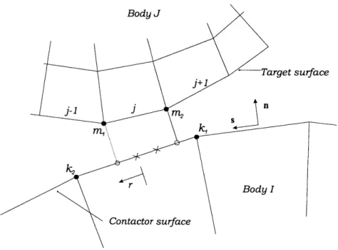
3-1 End nodes of target segment projected on contactor segment to create sub-segm ents. . . . . 39

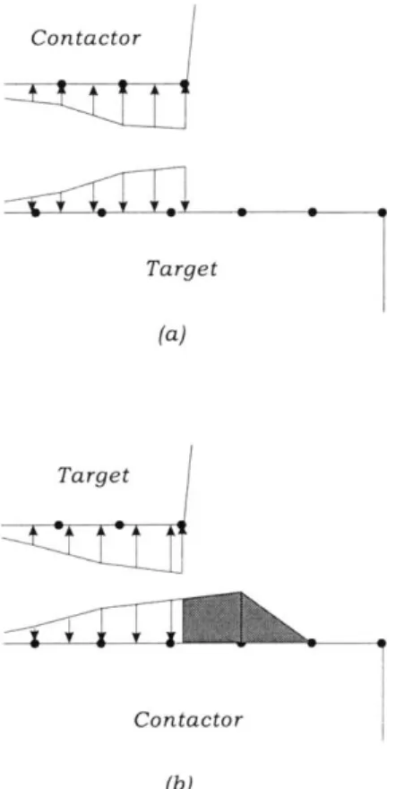
3-2 Choice of contactor and target surfaces; (a) top surface contactor, (b) bottom surface contactor. . . . . 44

3-3 _{The patch test. . . . . 46}

3-4 The patch test; oscillatory vertical displacement field obtained using the node-to-segment scheme. . . . . 47

3-5 The patch test; vertical stress field obtained using the node-to-segment schem e. _{. . . . 47}

3-6 The patch test; a uniformly linearly varying vertical displacement field obtained using the consistent segment algorithm. . . . . 48

3-7 The patch test; constant vertical stress field obtained using the consis-tent segment algorithm. . . . . 48

3-8 The patch test; incorrect displacement field using node-to-segment scheme; top block contactor. . . . . 49

3-9 The patch test; vertical stress field obtained using the node-to-segment scheme; top block contactor. . . . . 49

3-10 The patch test; displacement field using consistent segment scheme;

top block contactor . . . . 50

3-11 The patch test; vertical stress field obtained using the consistent seg-ment scheme; top block contactor. . . . . 50

3-12 The patch test; displacement field using node-to-segment scheme; top block contactor, 9-node elements. . . . . 51

3-13 The patch test; vertical stress field obtained using the node-to-segment scheme; top block contactor, 9-node elements. . . . . 51

3-14 The patch test; displacement field using consistent segment scheme; top block contactor, 9-node elements. . . . . 52

3-15 The patch test; vertical stress field obtained using the node-to-segment scheme; top block contactor, 9-node elements. . . . . 52

3-16 The elastic punch problem. . . . . 54

3-17 The elastic punch; horizontal stress field, using top and lower body as contactor. ... ... 55

3-18 The elastic punch; vertical stress field, using top and lower body as contactor. ... ... 55

3-19 The elastic punch problem; contact pressure distribution. . . . . 56

3-20 Hertzian contact problem. . . . . 57

3-21 Hertzian contact problem; horizontal stress field, 4-node elements . 58 3-22 Hertzian contact problem; vertical stress field, 4-node elements. . 58 3-23 Hertzian contact problem; horizontal stress field, 9-node elements . 59 3-24 Hertzian contact problem; vertical stress field, 9-node elements. . 59 3-25 Hertzian contact problem; contact pressure distribution. . . . . 60

3-26 Sheet in a converging channel. . . . . 61

3-27 Normal traction using 4-node elements; M = 0.0. . . . . 62

3-28 Normal traction using 9-node elements; yt = 0.0. . . . . 62

3-29 Tractions at times t = 4 and 8 s.; 4-node elements; p = 0.3. . . . . 63

3-30 Tractions at times t = 9, 10 and 16 s.; 4-node elements; [a = 0.3. . . . 63

3-32 Tractions at times t = 9, 10 and 16 s.; 9-node elements; it = 0.3. . . . 64

3-33 Comparison between CSA and NTS; t = 9 s.; 9-node elements; y = 0.3. 65

3-34 Comparison between CSA and NTS; t = 10 s.; 9-node elements; p = 0.3. 65

4-1 Convergence curve for the composite scheme. . . . . 73 4-2 Percentage period elongation and amplitude decay for the trapezoidal

rule, the Wilson method, the two sub-step composite scheme (-y = 0.5), and the original composite algorithm. . . . . 74 4-3 The rotating plate problem. . . . . 76 4-4 The rotating plate problem; results using the trapezoidal rule; At =

0 .0 2 s. . . . . 78 4-5 The rotating plate problem; results using the composite scheme; At =

0 .4 . . . . 79 4-6 The rotating plate problem; results using the Wilson 0-method; At =

0 .0 2 . . . . . 80 4-7 The rotating plate problem; results using the three sub-step composite

schem e; A t = 0.4s. . . . . 81 4-8 The compound pendulum in its initial configuration. . . . . 82 4-9 The compound pendulum; results using the trapezoidal rule; At =

0.005 s. . . . . 84 4-10 The compound pendulum; results using the composite scheme; At =

0 .0 1 s. . . . . 85 4-11 The compound pendulum; results using the composite scheme; At =

0 .02 s. . . . . 86 4-12 The compound pendulum; results using the composite scheme; At =

0 .04 . . . . . 87 4-13 The compound pendulum; results using the Wilson 0-method; At =

0.005 s. . . . . 88 4-14 The compound pendulum; results using the Wilson 9-method; At =

4-15 Cantilever beam modeled using 9-node elements . . . . 90

4-16 Cantilever beam; results using the trapezoidal rule; At = 0.002 s. .. . 91

4-17 Cantilever beam; results using the composite scheme; At = 0.004 s. . 92 4-18 Cantilever beam; results using the Wilson 0-method; At = 0.002 s. . . 93

5-1 Two impacting bars. . . . . 96

5-2 The displacements of contacting faces; trapezoidal rule, At = 0.00004 s. 97 5-3 The velocities of contacting faces; trapezoidal rule, At = 0.00004 s. . 98 5-4 The displacements of contacting faces; composite scheme, -y = 0.5, A t = 0.00008 s. . . . . 99

5-5 The velocities of contacting faces; composite scheme, y = 0.5, At = 0.00008 . . . . . 99

5-6 The total energy of the two bars obtained using the trapezoidal rule. 100 5-7 The total energy of the two bars obtained using the composite scheme. 100 5-8 The shaking table problem. . . . . 101

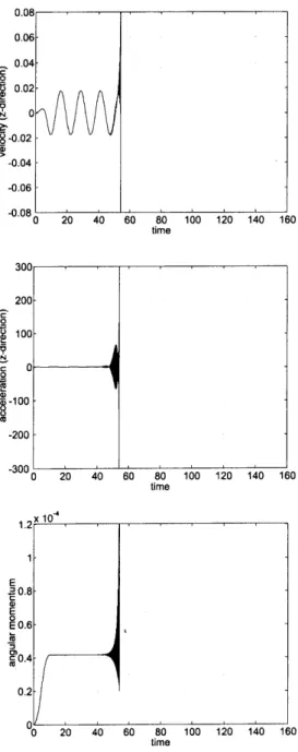
5-9 The velocity response of the table and the block; p = 0. . . . . 102

5-10 The displacements of the table and the block; p = 0 . . . . 103

5-11 The acceleration response of the block; p = 0. . . . . 103

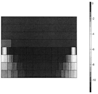
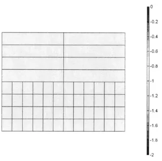
5-12 The normal contact distributions (for all time steps), 4-node elements; p = 0. ... ... ... .. .. . .. . . ... 104

5-13 The frictional contact distributions (for all time steps), 4-node ele-m ents; p = 0. . . . . 104

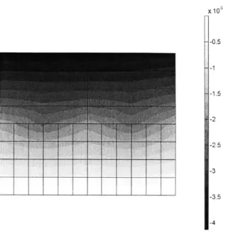
5-14 The normal contact distributions (for all time steps), 9-node elements; p= 0 . . . .. . . .. . . . . .. . . . . . . . . . . . 105

5-15 The frictional contact distributions (for all time steps), 9-node ele-m ents; p = 0. . . . . 105

5-16 The velocity response of the table and the block; p = 50000. . . . . . 106

5-17 The acceleration response of the block; p = 50000. . . . . 106

5-18 The normal contact distributions (for all time steps), 4-node elements; p = 50000. ... ... ... .. .... .... . 107

5-19 The frictional contact distributions (for all time steps), 4-node

ele-m ents; p = _{50000. . . . . 107}

5-20 The normal contact distributions (for all time steps), 9-node elements; p = _{50000. . . . . 108}

5-21 The frictional contact distributions (for all time steps), 9-node ele-m ents; p = _{50000. . . . . 108}

5-22 The velocity response of the table and the block; p = 35000. . . . . . 109

5-23 The velocity response of the table and the block; p = 35000. . . . . . 110

5-24 The acceleration response of the block; p = 35000. . . . . 110

5-25 The normal contact distributions (for all time steps), 4-node elements; p = 35000. . . . . 111

5-26 The frictional contact distributions (for all time steps), 4-node ele-m ents; p = 35000. . . . . 111

5-27 The normal contact distributions (for all time steps), 9-node elements; p = 35000. . . . . 112

5-28 The frictional contact distributions (for all time steps), 9-node ele-m ents; p = _{35000. . . . . 112}

6-1 Frictional sliding of a point mass. . . . . 115

6-2 Time functions governing the variation of applied loads. . . . . 115

6-3 Coulomb friction condition. . . . . 116

6-4 Regularization of Coulomb friction by constraint function. . . . . 118

6-5 The surface generated by the constraint function in Eq. (6.8). The thick line corresponds to wt = 0. . . . . 119

6-6 The derivative of wt w.r.t. t, a; for wt = 0. . . . . 121

6-7 The derivative of wt w.r.t. T, %; for wt = 0. . . . . 121

6-8 The trajectory of point A, under the action of applied loads; At = 1, Et = 10-5,

N

. . . .

6-9 Plot of incremental applied load vectors; At = . . . . 123 6-10 Plot of incremental friction force vectors; At = 1, Et = 10-5 , N = 1. . 123

6-11 Plot of incremental internal spring force vectors; At = 1, ct = 10-',

N = 1 . . . . 124 6-12 Plots of incremental load, spring force and friction force vectors at each

time step; the three incremental force vectors are in equilibrium. . . . 125 6-13 Comparison of the trajectory of point A, for different values of time

step size At; et = 10-'; (for total duration of 2 s). . . . . 126 6-14 Comparison of the trajectory of point A, obtained using At = 1 and

At = 0.1; (for total duration of 8 s). . . . . 126 6-15 Plot of incremental friction force vectors; At = 0.1, c, = 10-5, N = 1.

The circle shows the limiting value for the frictional force magnitude; at no time is this threshold violated. Points lying within the circle indicate a stick condition. . . . . 127 6-16 Comparison of trajectory of point A, for different values of Et; time

step size At = 0.1, N = 1. . . . . 129 6-17 Variation of normal force; N = 1 + 0.8 sin(20x) cos(20y). . . . . 130 6-18 Comparison of trajectories obtained; et = 10-, At = 0.1. . . . . 131

List of Tables

6.1 Convergence norms for some time steps; At = 1, ct = 10-5, N = 1 . . 128

Chapter 1

Introduction

Frequently in engineering analysis, there arise situations where in order to have an accurate solution of the problem at hand, actual contact conditions between structural

or solid elements have to be considered. Contact problems, by their very nature

are highly nonlinear, since not only the contact tractions are unknown, but also the surface area of the contacting bodies over which these act is also not known a priori. Among the many practical applications of contact analysis are soil-structure interactions, bio-mechanical engineering, metal forming processes, and crash analyses. For many applications it may be sufficient to consider frictionless contact, but in other instances the consideration of friction may be of utmost importance.

Numerical solution of contact problems is a difficult task, and efficient and robust techniques need to be utilized for reliable solution of general problems. Much research effort has been directed towards developing such schemes since early developments in the finite element method. Generally the techniques that are used to satisfy the contact conditions are the Lagrange multiplier method and the penalty method.

In the Lagrange multiplier method the contact conditions are satisfied by the

introduction of auxiliary variables, i.e. the Lagrange multipliers, which turn out

physically to be the contact traction variables at the contacting surfaces. The contact conditions are satisfied exactly, but the degrees of freedom now increase by the number of unknown contact traction variables, leading to greater computational effort. Bathe and Chaudhary [8, 14] presented an effective scheme based on this approach. The

Lagrange multiplier method transforms the problem formulation into a mixed method, and care needs to be taken regarding the optimality and stability of the method, i.e. the inf-sup condition has to be satisfied, see Brezzi and Fortin [13] for a detailed account regarding mixed methods in general, and Bathe and Brezzi [7] for contact problems in particular. Also for a comprehensive treatment of the Lagrange multiplier method and other optimization techniques see Bertsekas [12].

Penalty methods weakly enforce the contact conditions by introduction of a pa-rameter of large value into the governing equations of equilibrium for the contacting bodies. This penalty parameter acts like a large spring stiffness, see Bathe [3] and Zienkiewicz and Taylor [43]. The main attraction of the penalty method is that the total number of degrees of freedom remains unchanged. The contact conditions are enforced with increased accuracy as the penalty parameter goes to infinity. However there is a potential for ill-conditioning of the coefficient matrix as this limit is ap-proached. The approach has been used extensively, e.g. Oden [33]. Among recent works, the formulation based on mortar methods by Yang et. al. [42] utilizes penalty approach to satisfy contact constraints.

Augmented Lagrange methods combine both the Lagrange and penalty methods to regularize the contact conditions, see Kikuchi and Oden [25]. The approach has also been used for large deformation contact problems including friction, see for example Laursen and Simo [31]. Perturbed Lagrangian methods add a quadratic function of the Lagrange multipliers to the Lagrange multiplier term, see e.g. Simo et al. [37]. For a comprehensive survey of various techniques and algorithms for enforcing contact conditoins, see Wriggers [41] and the references therein.

In this thesis, a Lagrange multiplier based approach is adopted. A segment ap-proach first proposed by El-Abbasi and Bathe [18], is extended for solution of large displacement, kinematically nonlinear problems. The contact tractions are interpo-lated to the same order as that of the underlying continuum finite elements, leading to optimal convergence and stability, see El-Abbasi and Bathe [18] and Bathe and Brezzi [7]. The constraint function method first proposed by Eterovic and Bathe

This enables the algorithm to detect contact conditions while still away from contact event, allowing the use of larger time steps, see Eterovic [19].

1.1

Thesis Outline

In Chapter 2, the basic continuum mechanics equations including the contact trac-tions are presented. The physical constraints that are imposed by the presence of contact are given, including frictional effects. The constraint functions that are used to enforce contact conditions are presented. The constraint functions convert the in-equality constraints arising from contact conditions into in-equality constraints, and also regularize the non-smooth contact conditions at the same time. The contact integral that appears in the equation of principle of virtual work is linearized for subsequent application of Newton-Raphson method for the iterative solution. Detailed expres-sions for linearization of all the terms that appear in the contact integral is presented. The constraint equations which are obtained by multiplying the constraint functions by suitable weight functions are also linearized with respect to the unknown solution variables.

In Chapter 3, the scheme for projecting target segments onto contactor segments is given, along with appropriate finite element approximations for the contact surface and the contact traction variables. Expressions for finite element matrices obtained are also given. The chapter is concluded with numerical examples that show the performance of the algorithm.

Chapter 4 summarizes the difficulties usually encountered in the solution of non-linear dynamic problems using an implicit direct integration method. A simple but effective composite time integration approach is presented that produces stable solu-tions of nonlinear dynamic problems involving large displacements for long time dura-tions. The scheme performs well in instances where other widely used implicit direct integration methods exhibit instability. Numerical examples are solved to demon-strate the stability of the integration scheme.

using the contact solution algorithm given in Chapter 3, with the composite time integration scheme of Chapter 4. The stability characteristics of the time integrator also stabilize the solution at the instant of contact events, and it is observed that no special post processing of the response at contacting nodes is required. Large sliding response with friction, showing transition from stick to slip conditions, and vice versa, is also observed to be resolved accurately.

In Chapter 6 a model 3D friction sliding problem and its solution are considered. The constraint function method is used to enforce the Coulomb friction model. The problem is solved for different time step sizes, constraint function parameter values, and normal loads. Difficulties in Newton-Raphson convergence are observed and the use of line search in each iteration is suggested as a remedy to the problem.

Finally in Chapter 7 conclusions are given and possible future work regarding the contact solution algorithm is suggested.

Chapter 2

Contact Kinematics

2.1

Motivation

We seek to state the continuum mechanics formulation for the problem of elastic bodies coming into contact. More specifically, we will consider the case of two bodies coming into mutual contact, but extension to multiple contacting bodies is straight-forward and only involves the application of the formulations stated by considering each contacting pair successively.

The goal of the present work is to have a general formulation for bodies undergoing large displacements (and possibly large strains). The nonlinearity due to contact phenomena is due to the fact that the contact tractions at the interface are obviously not known a priori, but also because the actual contact area is unknown. The contact area can be dependent on the contact tractions and on the external applied forces driving the bodies to come into contact. Also large sliding can take place at the contact interface resulting in large changes in relative positions of points lying on contacting surfaces. It is of great importance that the kinematics of all the varying quantities at the contact interface be considered and included in the formulation, to capture the correct behavior. For a more general treatment, see Wriggers [41]. In the following sections we state the contact kinematics with reference to 2-D contact between two bodies, and enforce the contact constraints by means of the constraint function method, Eterovic and Bathe [21]. Also, to solve the nonlinear problem,

one has to use an iterative procedure for the solution of resulting equations. Full Newton-Raphson method will be employed, which converges quadratically to the exact solution, provided the required conditions of smoothness and continuity are satisfied, see Bathe [3] and Bertsekas [12] for details. For this reason, it is necessary that all kinematic variables be linearized exactly, so that consistent tangent stiffness matrices can be obtained and the quadratic convergence property can be utilized.

2.2

Continuum Mechanics Equations

In this section the general continuum mechanics equations for bodies coming into contact are presented. Although, in general more than two bodies can come into mutual contact, in the following we consider the case of only two bodies. All the discussion is also directly applicable for multi-body contact, with kinematics of each contact surface pair treated in the same manner as given in this chapter.

We consider two bodies Q, i = I, J, which are in contact at time t. For each

body, S, is the surface over which Dirichlet boundary conditions are specified, and

Sf the surface with Neumann boundary conditions. We denote by S' the surface area

of body I that can come into contact with body J, and Sj the surface of body J that can potentially be in contact with Sj. Together SI and Sj make a contact surface pair. Let tSc be the actual contact area common to both S' and Sj at the time of consideration. Following the approach in Bathe[3] the principle of virtual work for the two bodies is:

Find 'u E V where V is defined as

'{J

S -6

d}V

ud 'tV

tis,

u s

dtS

+ tfJ- (Juj -

6u') dtS

JtSc

the contact integral

Body J

su

Figure 2-1: Two bodies in contact.

V = {vlv E H1

(Q),

where n is a normal unit vector to be defined, and go is a possible initial gap. The left hand side of the above equation represents the total internal virtual work, expressed in terms of second Piola-Kirchhoff stresses and the Green-Lagrange strains calculated at time t. The first integral on the right hand side is the total external virtual work done by the body forces and any externally applied surface tractions. The second integral on the right hand side is the contribution from the contact tractions which

act on both the bodies over the surface 'S, in equal and opposite directions. tf JI is the

vector of contact surface tractions acting on body J due to body I. Over the surface

of contact we have from the principle of equal and opposite reactions fIJ -tfJI.

This results in the compact form of the contact integral in the above equation. In the following discussion we are only concerned with the evaluation of the contact integral since this is the key step in the evaluation of contact tractions and displacements of

the contacting bodies. We designate surface S' as the contactor and surface Sj as

the target. Also 'f JI is replaced by Tfc in the following discussion. In a continuum setting, it makes no difference now, whether the contact integral is evaluated over the target surface or the contactor surface since the actual area of contact 'Sc at time t is the same no matter which surface is chosen. For a discretized problem, of course

there is a bias introduced depending on which surface is chosen for integration. In this work, the contactor surface S' is chosen as the surface over which the contact integral will be evaluated.

Let s be the tangent vector at a point on SI. Then the unit normal n is defined over S' such that n and s form a right hand basis

n = s x e (2.2)

where e is the unit out of plane vector. Now the vector of contact tractions acting on S' can be decomposed as

'fC = An + ts (2.3)

We refer to a point by its position vector in the following discussion, see Figure 2-2. In order to define the signed distance from a point x, on contactor surface S' to the target surface S', we solve the following expression for xj

(xj - x') - s = 0 (2.4)

then

gn = (xi - x') (2.5)

The signed distance or gap function is now given by

g = (x' - x') . n (2.6)

We parameterize the contactor surface by a local variable r and evaluate the variation of the gap function as follows

wg = (dxoe - x - xabr) - n + (x - x) - n (2.7)

target

X -X

n r

contactor X

Figure 2-2: Contact kinematics of contact pair.

6g = (6xj - 6x') - n (2.9)

The above expression results due to the fact that 6n I n and x' I n. Note that I.r

x X,r is a tangent vector and we use a, ist vcoreuea.=vco x'. To obtain the unit tangent vector the following relation is used,

s= (2.10)

||ar l

Substituting the expression for vector of contact tractions from equation (2.3) into

the contact integral on the RHS of(2.1) and noting that 6x' = 6u', we can write

I fJ -(6uj - 6u') dS = A6g dS +

j

JSI I

JSI

With the expression for contact integral in hand, we now proceed to state the contact conditions at the interface surface. For normal contact, the essential condition to be satisfied is the condition of zero inter-penetration of the contacting bodies. Also the contact tractions are such that there is zero adhesion between the bodies. These conditions can be written as a set of Kuhn-Tucker equations

g > 0

A > 0 (2.12)

gA = 0

com-X.

+1

g

u

-1

Normal contact conditions

Tangential contact condition

Figure 2-3: Contact conditions.

To take into account the frictional contact conditions, Coulomb's law of friction is assumed to hold point-wise, with p being the coefficient of friction. Define the non-dimensional variable T as

__t

r =(2.13)

pA

and the magnitude of the relative tangential velocity corresponding to the unit tangent vector s at xi as

it

(n, -

nj)

- s

(2.14)

Coulomb's law of friction can then be stated in terms of the following conditions

17- < 1 it

n

(2.15)

TI

1

sign(it)

The solution of the equation of virtual work (2.1) subject to the above normal and tangential contact constraints results in the solution of the contact problem

2.3

The Constraint Equations

We choose to enforce the contact conditions given in equations (2.12) and (2.15) on the principle of virtual work given in equation (2.1) by means of Lagrange multipliers,

which are really the normal contact pressure A for normal contact and the non-dimensional variable r for the frictional contact. The constraint function method given in Eterovic and Bathe[21] regularizes the contact constraints and at the same time reduces the inequalities in these constraints to a set of equality constraints which can be solved for using the standard Lagrange multiplier approach. The method is also very attractive since the constraint functions provide information to the algorithm about the changes in contact conditions while still far from convergence. Therefore relatively larger time steps can be used, as compared to the conventional active set strategies used for inequality constraints.

Let w,-, be a differentiable function of g and A, such that the solution of wn(g, A) = 0 satisfies the normal contact conditions in (2.12). Similarly, let w, be a function of

it and T such that the solution of w,(it, T) satisfies the tangential contact conditions

in (2.15). This reduces the inequality contact constraints, to the following constraint equations

wn(g,

A)

wT

(u,

r)

0

(2.17)

Let Ec and c, be small, real and positive numbers, and

A(g)

9

2

r(,t) = arctan

-

The function wn is now obtained by generating a surface by passing a line with direction (1, 1, 1) corresponding to (g, A, wn) along the curve A(g). Similarly w, is obtained, in an implicit form, by passing a line with direction (1, -1, 1) corresponding

0.8 0.6 0.4 0.2-w,(g,X) __ _ _ _ _ _ _ _ _ _ _ _ _ _ _ _ _ _ _ 0 0.2 0.4 0.6 0.8 1 g

Figure 2-4: Constraint function for normal contact.

to (it, r, w,) along the curve T(i)

Wn(g, A) = 2 2 A) + n (2.20)

T + w, = 2 arctan -W (2.21)

7r Er

Multiplying equations (2.16) and (2.17) and integrating over the whole surface S', we obtain the constraint equation

I [6A Wn(g, A) + Tr w,(iL, T)]dS' = 0 (2.22)

Now the principle of virtual work can be solved for the two-body contact problem subject to the above constraint equation which provides the information about the contact conditions at the interface. The unknowns in this set of equations are the displacements of the bodies and the unknown contact forces expressed in terms of A and r.

T

w (u,T) _U

-1 1

Figure 2-5: Constraint function for tangential contact.

2.4

Linearization of the Contact Integral

The principle of virtual work given in (2.1) and the contact constraint equation (2.22) are nonlinear in displacements and contact tractions. The term representing the in-ternal virtual work in terms of second Piola-Kirchhoff stresses and Green-Lagrange strains can be linearized in the usual way, see for example Bathe [3]. Even if the prob-lem is kinematically linear, the presence of the contact terms still makes the equation nonlinear. For finite element solution of nonlinear problems in computational me-chanics, the Newton-Raphson method, which is quadratically convergent, is widely used. But to take full advantage of the quadratic convergence of the method, the nonlinear equations have to be consistently linearized. In the following discussion we focus on the linearization of the normal and tangential contact terms in the contact integral in (2.11) individually to simplify the presentation, and follow a approach similar to that used in Wriggers [41].

2.4.1

Linearization of Normal Contact

The normal contact term in (2.11) at time t

+

expansion about the state at time t, with second order and higher terms dropped, as

t+At A6g dS=

j{

(2.23)

s(

s(

A)

j

j{

where AA is the increment in the normal contact traction and A~g is the increment in the variation of the gap function. To evaluate the term A~g in terms of incremental displacements Au, we need to go back to the definition of the gap function in (2.5). We cannot compute Acg directly from (2.9) since the terms which turned out to be zero in evaluation of 6g can still contribute to Adg. Therefore we start by taking variation of each term in (2.5) using the fact that local variable r parameterizes the

contact surface so that xi = x'(r), and 6x' = 6u', 6xj = Juw

Juj - Ju' - x Jr = 6gn

+

If the above equation is multiplied by n we will get the expression for 6g same as (2.9). We employ the idea of directional derivatives directly to above equation and

later simplify for A6g. By taking increments of each term in (2.25), and noting that

Axi = Au we have

-[JuAr + Aul,6r + x',, Arr + X A6r] = A6gn + JgAn

+

+

Taking the dot product of each term in the above equation by n, the expression for

Adg is obtained

In this expression for Adg the quantities 6r,Ar and Aon are still unknown. We first establish an expression for Jr as follows. From the fact that (xi - xI) I ar, where a = x',. is the tangent vector at x, we have

(x'i -

-a, = 0

(2.28)

Taking the variation on each term in this expression we obtain 1

Jr = (2 -)[(Ju - Ju') -x, + gn - u,.] (2.29)

(12-- gn - xI,,)

where

2

I

(2.30)

The structure of the term Ar is the same as above except that variations are replaced by increments,

1

Ar (2 [(AuJ - Au') -x, + gn - AuI] (2.31)

(12- gn -XI,,r)rr

The term Aon - n can be evaluated using the fact that Jn I n,

Jn - n = 0 (2.32)

A(Jn - n) = 0 (2.33)

and hence

In order to computer the variation and increment in the normal vector n, use is made of the orthogonality of n with the tangent vector ar = x

n - ar = 0 (2.35)

6n - a, = -n -6ar (2.36)

(Jn - a,)a, = -(n - 6ar)a, (2.37)

(1n s)s = (n

-

The relation n _L 6n implies 6n 11 s which simplifies the above expression to

n = ( - a)a, _(2.39)

The increment of unit normal n is computed similarly and has the same structure, increments replacing variations

An

_{(n -Aa,)a,}

_(2.40)

In the above expressions for variations and increments for normal vector n

6a, =6u,.+ x', 6r and Aar = Au'

+

Substituting expressions from (2.34), (2.39), (2.40) and (2.41) into equation (2.27), the general expression for A6g is obtained as follows

Adg = - [6u,.Ar

+

+

9 r(2.42)r

+2

(6u',.

-

With the above expression the linearization for the normal contact term in (2.24) is complete.

2.4.2

Linearization of Tangential Contact

In order to treat the tangential contact term in (2.11), consider first the following expression which follows directly from the orthogonality of x- - xI = gn to the tangent vector;

(xi - x') - ar = 0 (2.43)

Taking variation of each term

(6u' - 6u, - x',6r) - a

+

1Or

where we used the fact that for tangential contact to be active, the term xj - x, = 0. The tangential contact term at time t + At can be written in terms of a Taylor expansion about time t as follows, keeping in mind that t = LAr

j

j

{

+

_t

_A[(6u'

_-

_-u')

_s]

(2.46)

+

± tG(6uJ - 6u') ts [LtAA} dS

The first term on RHS is easy to compute since all the terms depend on the known configuration and the current contact tractions which are assumed to be known. The third and fourth terms on RHS are also trivial to compute once the problem has been discretized and suitable interpolation for contact variables is chosen. It is the second term which needs to be evaluated carefully to obtain a consistent tangent stiffness. Considering equation (2.45) and taking increments

A(16r)

lA~r

Alr

A[(Juj

6u')

Comparing the above equation with (2.46), it is clear that once expressions for ALr and Allr are evaluated, the linearization of the tangential contact term is complete.

In order to find Ar, consider once again equation (2.26)

-[u,.Ar + AuQJr + x,,Aror + x',. Ar] = ALgn + 6gAn + Agon + gAon (2.49)

Taking the dot product of each term in this equation with the tangent vector ar and rearranging the terms, the following expression is obtained,

-12Ajr = (6gAn + Agon

+

+

+

In order to simplify the third term on the RHS of the above equation consider the orthogonality condition

n - ar = 0 (2.51)

J(n - a,) = n - ar

+

AL(n - a) = A6n - ar

+

+

+

Adn - ar = -(Jn - Aar

+

+

where

Ad, [Jui,

+

A~ar = r ±rr ](2.55)

urAr

+

+

expression making use of the relation for Aon - a, from above equations, (JgAn + Agon + gAon) - a,

= (JgAn + Agon) - a, - g(Jn - Aa, + An - Ja,) - gn - A6a,

= JgAn- a,

+

= -Jgn- Aa, - Agn - Ja, - gon -Aa, - gAn -a, - gn - Ada,

= -[6(gn) - Aa,

+

= -[6(x - x') Aa, + A(xj - x') - a,] - gn- Ada,

= -(6uw - Ju)- Aa, - (Auj - Au') - a, + x', Jr -Aa, ± x',Ar - a, - gn - Ada,

(2.56)

With the above equation substituted in equation (2.50), and some rearrangement of like terms, the following expression for Adr is obtained

Aor = [(u-' - Ju') - Aa + (Auj - Au') - Ja

- a,- (6rAu',

+

- (a,.. x',, - gn -x',,,.)drAr

+ gn- (u'~,.Ar + JrAU,.) (2.57)

- Jra, - (AuI + xi ,Ar) - (u!', + xfr,,r) aAri-1

(12 _ gn -X!,,)

In this expression Jr and Ar have to be substituted by expressions in equations (2.29) and (2.31). This results in an equation which, although very complicated, is completely linear in terms of the increments in displacements, Au. It is interesting to note that the above expression is symmetric with respect to du and Au, and hence results in a symmetric contribution to the tangent stiffness matrix.

To evaluate the expression for Aldr, recall that

Taking increments on both sides,

I

Al = (a, - Aar) (2.59)

the required expression is obtained

Al6r = (ar - Aar) (2.60)

It is instructive to note that this expression is non-symmetric in the variations and increments of the unknown displacements of the contacting nodes, and will result in a non-symmetric contribution to the tangent stiffness matrix.

2.5

Linearization of the Constraint Equations

The constraint equations given in the last section can be linearized similarly to obtain expressions which are linear in incremental displacements and incremental contact

tractions. Writing the constraint equation (2.22) at time t

+

about time t with only first order terms, we obtain

J {19W+ Ag + "aA}

s [6AXW+ 1

ag

A

+ 6T{t_{w+ a}

_{An+ 1 Ar} dS = 0}

In this linearized equation all the terms can be computed with relative ease. Ag is computed similar to 6g as in (2.9),

Ag = (Aug - Au') - n (2.62)

The new term in the linearization of the constraint equation is the increment in the relative velocity Az! which needs to expressed in terms of incremental displacements Ax. For this a numerical approximation to velocities need to be made: here we make

use of a backward difference approximation,

n

(2.63)

With this approximation made for velocities, the increment in relative velocity is computed easily in terms of incremental displacements as

A -= A[(n' - i) - s]

= I

[Auj

where

1

As

[Au',

a

_Al

Chapter 3

A Consistent Segment Algorithm

(CSA)

3.1

Motivation

Having stated the continuum mechanics equations in the previous chapter, the next step in the numerical solution of contact problems is to discretize the continuum and the contact surface variables. Finite element discretization is almost universally employed for solution of problems in solid mechanics, and it is not the goal of this thesis to present a detailed account of the method. Refer to Bathe [3], Strang and Fix [38] or Ciarlet [16] for a detailed treatment of the topic.

Numerical solution of contact problems, however, is a different story. There are

various approaches that have been employed to date. These approaches can be

broadly categorized in three classes : node to node, node to segment, and segment to segment approaches. A segment algorithm which is stable and consistent with the fi-nite element discretization of the continuum, was proposed and implemented for small displacement analysis in El-Abbasi and Bathe[18]. In this chapter we present the al-gorithm for general, large displacement analysis of contacting bodies. The Lagrange multiplier approach is employed, using the constraint function method.

3.2

Finite Element Discretization

Once a finite element discretization for the continuum is chosen, the discretization that follows for the contact surfaces is kept to be consistent with that of the con-tinuum. This is one of the key ingredients of the proposed contact algorithm, and with careful treatment, enables a consistent transfer of contact traction to each of the contacting surfaces irrespective of the choice of contactor and target surfaces.

The geometry of the contactor surface, discretized by p-node segments is interpo-lated as

p

x' hcxf (3.1)

i=1

where h, and xf are the interpolation function and the position vector for the node

i, and he, = hes(r), r E [-1,+1] being the local variable parameterizing a given contactor segment. The incremental displacements of points on the contactor surface are interpolated to the same order (isoparametric discretization), using the same shape functions,

p

Au'= heAuf (3.2)

i=1

Similarly for, target surface, discretized by q-node segments,

q x' =Zhtxj (3.3) j=1 q Au =

Z

where ht, = ht3 (r*), r* being the local variable parameterizing the target surface.

Let Aft be the vector of length 2(p+q) containing incremental node displacements for both contactor segment and target segment nodes,

etfiT entries re dth u1 Au1 ... noU AU (3.5)

entries to target segment nodes. Similarly for variations of nodal positions,

6&X Yu Y. X Yp3~ ... Xu ouY (3.6)

We can now express Auj - Au' in terms of interpolation functions as

Auj - Au'= H An (3.7)

where

he, 0 ... h 0 ht, 0 ... h 0

H = (3.8)

0 - he, ... 0 - he, 0 ht, ... 0 htq

Similarly Au,, can be written in terms of the vector of incremental nodal

displace-ments, and interpolation matrix H of size (2 x 2(p

+

Au', = H ,n (3.9)

with

he

0

..

he

0

i

0

...

l

H,Cpr ... (3.10)

0

hc,.r

The last 2q columns of the matrix H, are zero since these correspond to the target segment nodes, the interpolation functions ht, of which are not functions of the local

variable r which parameterizes the contactor surface SI. Similarly, Au, = H,,. An,

which is required in the formulation for 3-node contactor segments, where H,,r is a matrix holding second derivatives of contactor surface interpolation functions.

The variations in displacements are chosen from the same finite dimensional sub-space of admissible functions, giving the following equations

and

,r r= H, 6n (3.12)

The contact tractions have to be discretized along the contactor surface as well. As shown in El-Abbasi and Bathe [18] and Bathe and Brezzi [7] We choose the same interpolation order for approximating the contact tractions between nodal values, is the interpolation order chosen for the spatial discretization of the contactor sur-face. For a given contactor segment with p nodes, the normal contact pressure and tangential contact traction can be written as

\= H, A (3.13)

T =

Hc1r

_(3.14)

where the 1 x p matrix H, contains the p interpolation functions he,, and A and r p x 1 vectors containing the traction values at contactor segment nodes,

Hhpl

[

-

- he,

(3.15)

A,..ApI

..

(3.16)

3.3

Consistent Segment Algorithm

With the finite element approximations stated in the previous section, we are in a position to write down the finite element equations of the whole system, in which the incremental nodal displacements of the contacting bodies, and the incremental contact tractions at the contactor nodes are the unknowns to be solved for. The finite element equations are obtained in a standard way by using the finite element approximations in the linearized equations obtained in Chapter 2. The unknowns are the incremental nodal displacements and contact traction variables. This requires the evaluation of integrals over the contactor segment.

Body J -Target surface j+1 j-1 k2S r _BodyI Contactor surface

Figure 3-1: End nodes of target segment projected on contactor segment to create sub-segments.

For non-matching contact interfaces, the target and contactor nodes do not match, and the expressions arising in the linearization of the contact integral, Eq. 2.11 are not continuous. It is evident from Figure 3-1, which shows the case of linear elements, that the gap g though continuous will not have a continuous derivative. This poses a problem in the evaluation of integrals. The consistent segment algorithm circumvents this obstacle by further subdividing a contactor segment, into sub-segments, over which the gap and its derivative, both are smooth. Figure 3-1 shows a case of linear

contactor and target segments. The nodes m, and m2 of the target segment j project

onto the contactor segment with end nodes k, and k2. This creates sub-segments

on the contactor segment (in this case three), and all the integrals arising in the calculation of the finite element equations can now be evaluated sub-segment wise, and summed. Note that while evaluating the two sub-segments at each end of the

contactor segment, the corresponding target segments are j

+

j

The finite element approximations given earlier when used in evaluation of the linearized contact integral obtained in Chapter 2, gives rise to the following finite

element equations for incremental displacements and contact traction variables.

tKu

tKuu

tRc _(3.17)

tKcu tKcc Ai TFc

The first row in this matrix representation is obtained from the principle of virtual work after nonlinear terms have been linearized, and the second equation (row) cor-responds to the linearized constraint equation which imposes the contact conditions on the system. The terms in these equations are evaluated using the most recent con-figuration, obtained during a Newton-Raphson iteration while solving for unknown variables at time t

+

t+AtR is the vector of externally applied forces at time t + At. F is the vector of internal forces calculated using the most recent displacement configuration. tRC

is the vector storing the nodal forces due to contact tractions. The stiffness matrix contribution tKas is the gradient '. The rest of the matrices and and vectors are obtained using the finite element interpolations given above in the linearized equations of Chapter 2. In the following we give the relations to compute these matrices for the case of 2-node contactor and target segments. In this case all the second derivatives and higher, with respect to the local parameter turn out to be zero within each contactor segment. Let there be total N contactor segments, with each segment having n subsegments once all the target segment end nodes have been projected on the contactor surface. The number n may be different for each contactor segment. Also in all subsequent integrals, we assume unit magnitude thickness.

The vector of nodal forces obtained from contact tractions is then,

tRC

=

HT(An +

ATs)

det JScdr

(3.18)