A. MULTIPATH TRANSMISSION
Prof. L. B. Arguimbau W. L. Hatton G. M. Rodgers Dr. J. Granlund E. E. Manna C. A. Stutt
R. A. Paananen 1. Speech and Music
a. Field-test receivers
Field tests on transatlantic transmission have been in progress for about two months at time of writing. Unfortunately the frequency (26 Mc) assigned to us proved too high for the existing ionospheric conditions and transmission has been unsatisfactory. The reception is almost exclusively on random scattering, and the resultant is noisy and the repair circuits have been ineffective. Tests are now in progress on 23.09 Mc.
J. Granlund, C. A. Stutt 2. Television
An effort to determine the relative performance of the present system of video transmission with frequency modulation has been under way for a long period. Recently this work has been accelerated. In order to avoid the purchase of camera equipment and to simplify the circuitry it has been decided to carry on preliminary work using a scale model based on a facsimile system. The time scale is stretched by about 104 A line period is now about 0.6 sec, the time taken for a sound wave to travel 700 feet. This makes it possible to get fractional-line delays by the use of an acoustic tube about 60' long. A block diagram of the system is shown in Fig. VIII- 1. The various com-ponents.are now complete except for the delay line, and it is hoped that information on the operation will be available by the next quarterly report.
L. B. Arguimbau, W. L. Hatton, E. E. Manna, R. A. Paananen, G. M. Rodgers
Fig. VIII--- Block diagram of frequency-modulated facsimile test circuit.
Fig. VIII-l Block diagram of fre quency- modulated facsimile test circuit.
850 pulses per second;
AT
=
1.1 sec.
B. STATISTICAL THEORY OF COMMUNICATION
Prof. J. B. Wiesner
Prof. W. B. Davenport, Jr. Prof. R. M. Fano Prof. Y. W. Lee Prof. J. F. Reintjes Dr. O. H. Straus B. L. Basore R. S. Berg J. J. Bussgang L. Dolansky P. E. Green, Jr. B. Howland L. G. Kraft A. J. Lephakis H. Levick F. L. Petree C. A. Stutt D. E. Ullery I. Uygur1. Single-Channel Analog Correlator
The analog correlator has been placed in operation, and considerable time devoted
to a study of its operating characteristics.
In its present form the machine provides
110 points on the auto- or crosscorrelation curves of signals lying within the frequency
range of 500 cps to 100 kc.
The lower frequency limit is determined by the maximum
available delay between pairs of sampling pulses (2.5 msec), and the upper frequency
limit is fixed primarily by the sampling-pulse width (1.5 Isec).
Either 8, 000 or 16, 000
samples may be taken at rates between 300 and 1000 samples per second.
Figures
VIII-2 to VIII-5 are examples of results obtained with the machine, and show the form
in which data are presented.
..
..
..-.
Fig. VIII-4 Autocorrelation curve of a 2-kc rectangular wave.
Sampling rate, 300 pulses per second; AT = 174sec.
- m . m
I
X f I I i
--- -
---Fig. VIII-5 Crosscorrelation curve of a 3-kc rectangular wave synchronized with a 3-kc sawtooth wave. Sampling frequency, 500 samples per second; AT = 9 sec.
The correlator is being built into a more permanent form suitable for a tea-wagon type of mounting. Details of the circuitry of the correlator are to be included in a
forthcoming report. J. F. Reintjes
2. Multichannel Correlator
Work on this project is centered on three components: the development of a master-pulse generator, a narrow-master-pulse sampling circuit, and an output circuit which will permit the signals from the various channels to be displayed simultaneously on a cathode ray tube screen. It is expected that most of the circuitry involved in these components will have been worked out by the end of the next quarterly period.
Y. W. Lee, J. F. Reintjes, D. E. Ullery, F. L. Petree, H. Levick 3. Digital Electronic Correlator
The correlator has been used to detect the waveshape of a periodic signal in the presence of noise and a second, larger, periodic signal which differs in frequency from the first by only a few cycles per second. Figure VIII-6 shows the relative amplitudes
of the three components of the signal fed to the correlator.
The sawtooth, noise, and square-wave are added together producing the result shown in Fig. VIII-7. Although the sawtooth is masked by the noise and by the large square-wave, crosscorrelating this combined wave with a periodic unit impulse of the same frequency as the sawtooth results in a curve having the same shape as the
b
c
Fig. VIII-6 Components of correlator input (a)
sawtooth-wave; (b) noise; (c) square-wave.
Fig. VIII-7 Input to correlator (sum of waves
inFig. VIll- 6) .
I ~ -..J I a bamplified version of the sawtooth for comparison. In this experiment: Sawtooth frequency = 31, 250 cps
Square-wave frequency - 31,255 cps
T shift between two lines on crosscorrelation curve (AT) = 2
psec
Number of samples of noise = 30, 720 Number of samples of signal = 15,360
Y. W. Lee, L. G. Kraft, I. Uygur 4. Pulse Code Magnetic Recorder
The six-element Tchebycheff-type filter, designed to attenuate frequencies higher than 10 kc at the input and having an impedance level of 1.5 kilohms, has a transfer characteristic meeting this requirement very well. However, it was found difficult to obtain the same transfer characteristic when the filter was connected to the source. In some cases the source was affected by the frequency-sensitive parallel load presented by the filter input impedance; in other cases the maximum signal voltage had to be
reduced to a fraction of a volt in some part of the channel and this resulted in hum troubles. (If 1/128 of the maximum signal voltage is of a size comparable to the hum
voltage, the least significant digit of the pulse code becomes useless.)
A satisfactory solution was obtained by carrying out the following three steps: (a) The impedance level of the filter was increased to about 20 kilohms (i.e. as far as readily available inductances permitted; this allows a corresponding increase in the cathode resistance.
(b) A high-current tube was used for the cathode follower (both halves of 5687), so that with a given cathode resistance a much higher voltage is developed across the cathode resistance.
(c) The following phantastron stage was changed so as to require only 68 volts peak-to-peak. It should be mentioned at this point that this last change makes it easier to obtain linear amplification with a 300-volt supply, but does not solve the hum problem.
The diagram of this arrangement is given in Fig. VIII-9, the over-all response in Fig. VIII-10, and is essentially the same as for the filter alone.
Several changes have been made on the mechanical unit. A new recording-and-playback head was obtained from Raytheon Manufacturing Company and is being mounted onto the driving mechanism. Various parts of the latter are being overhauled to ensure a smooth run of the tape in the region of the recording-and-playback head.
The problem of compression and expansion of the audio signal and the scheme represented by Fig. VIII-11 is being investigated, to see whether a Logaten logarithmic attenuator could be used for the magnitude sensitive gain P(v) in the expander and com-pressor. The additional gain K1 will be necessary because the maximum output of the
attenuator is of the order of 0.1 volt.
5687 IOK OUTPUT mh 750mh 750mh O. If IN 560 662 Hyf 4.3 K
Fig. VIII-9 Cathode follower with filter and amplifier.
COMPRESSED I AUDIO AUDIO (o) K COMPRESSOR 100 looo 10,000 TO 91.81 -6SN7 2 I0 CODIN( PLAY G, RECORDING BACK AND EXPANDER
F
interference have been encountered. A new model, which would minimize these troubles through the use of a pentode gating scheme, is being tested at the present time.
J. B. Wiesner, L. Dolansky 5. Felix (Sensory Replacement)
The series of experiments outlined in the Quarterly Progress Report, January 15, 1951, is being continued, with emphasis on methods of analysis of the binary signals intended for tactile stimulation. A method for determining the first conditional proba-bility distribution of the binary signals involving time exposures of these data mapped on a cathode ray oscilloscope, is being tested. This measurement should make possible a more accurate calculation of the information content of these signals, and may also provide a convenient display of the complex statistical structure of a sample of speech; tests with different speakers and different languages are also planned. In conjunction with the use of the Vocoder for speech analysis and synthesis, experiments were under-taken to enable synthesis of speech from short-time autocorrelation function signals;
results will be reported. J. B. Wiesner, O. H. Straus, B. Howland
6. Amplitude Distributions of Filtered Speech
The first-probability distribution densities of instantaneous conversational speech amplitudes in adjacent frequency bands, covering the frequency range from 160 cps to 9000 cps, are being determined with the aid of the probability distribution analyzer.
The speech sources used in these tests are the separate recordings of the voices of three people while reading from the same passage of a magazine article in an anechoic
space. The filtering is being accomplished by means of a set of adjacent band pass filters, whose bandwidths are each 250 pitch units wide.
The results of these measurements will be used in an attempt to substantiate pre-vious data on the distribution of rms speech amplitudes (H. K. Dunn, S. D. White: J. Acous. Soc. Am. 11, 278-288, Jan. 1940) which have been used as one of the founda-tions for the development of articulation indices as a quantitative measure of the
intelli-gibility of speech sounds in the presence of noise.
W. B. Davenport, Jr., R. S. Berg 7. Brain Wave Investigations
Our conclusions about the nature of "kappa" rhythm have been verified by a repetition of the previous experiment. The original question was whether the apparent phase
opposition of the characteristic 8 cps signals observed between each temporal lobe and the chin was due to propagation time from one side to the other, or whether two signals were generated simultaneously but with opposite polarities. Figure VIII-12 is a typical crosscorrelation curve; the corresponding cross-power density spectrum, Fig. VIII-13,
z12 IN 3 ARBITRARY
UNITS 2
180 r IN MILLISECONDS
Fig. VIII-12 Crosscorrelation of "kappa' wave from opposite temporal lobes. (Central peak caused by pickup and muscular activity common to both channels.) T
(T) = Lim
1
f
+ T)
dt
T- 2T fl(t) f(t + T)dt -Twhere fl(t) = voltage
f2(t) = voltagebetween right temple and chin
between left temple and chin.
135 180 225 1.5 0.5 I I I 6 8 10 FREQUENCY - CYCLES/SEC I - J 12 14
Fig. VIII-13
shows a phase angle of about
original brain waves were of
have been characterized by a
zero for zero frequency.
Cross-power density spectrum 1 2(w) derived
from 1 2(T) of Fig. VIII-12 by a Fourier transformation.
180' irrespective of frequency. This means that the two opposite polarity. A delay due to propagation time would
phase angle increasing in proportion with frequency and
P. E. Green, Jr. with J. U. Casby of Massachusetts General Hospital
IC. HUMAN COMMUNICATION SYSTEMS*
Prof. A. Bavelas J. B. Flannery D. G. Senft
F. D. Barrett R. D. Luce P. F. Thorlakson J. Macy, Jr.
1. Experiment on Network Patterns and Group Learning
The experiment is proceeding as scheduled. We are using as subjects groups of five men provided by the First Naval District Headquarters from their pool of transient Navy personnel. In general, we are able to run ten groups a week except on occasions when the pool of men is for some reason markedly reduced. When this work is
com-pleted and the data analyzed a fuller report will be given.
F. D. Barrett, R. D. Luce
2. "Octopus"
The five operating panels and the control section of "Octopus" have been completed and tested. The recording section is under construction and it is hoped that it will be completed in the near future. It is proposed that during the coming weeks we use
groups of people to test the equipment as an experimental tool. It is expected that these tests will result in an adequate knowledge of the most effective way to use this equipment and that they will lead to the design of a specific experiment for its use. Further detailed description of the apparatus and its proposed use in an experiment will be given when
these trials are completed. J. Macy, Jr.
3. A Study of the Problems of Recognition and Linguistic Encoding of Complex Patterns
The first-order information which flows among the members of a task-oriented group is defined as information that pertains to the external state of affairs to which the group is attempting to adapt. This external state of affairs can be physical or social, and either structurally simple or complex. Because the group has to have information about this state of affairs if it is to make decisions and to act, there will of necessity be at least one link which extends between the external happenings and the group itself. If this external state of affairs or pattern of information has a number of elements and falls into a complex set of temporal and physical relationships, it may be difficult for the observing group member to grasp the structure of the pattern or, if he does, to translate his perceptions into language or other code. This is especially true of patterns
which are distributed not only over space but also over time. One can think of many social groups whose communication links with the environment must deal with the problems of complexity of pattern.
"READY" LIGHT
/ COPPER LATTICE
P DOOR
P DOOR
Fig. VIII- 14
Testing device for pattern recognition.
SELECTOR SWITCH
"WIN" LIGHT -"READY" BUTTON
COIN BOX CONTROL BOX
The present investigation proposes to undertake exploratory studies of this problem using an apparatus which has been designed for this purpose by Josiah Macy, Jr. and John Flannery. The study will consist of two phases: (a) an investigation of the ability to recognize patterns and (b) an investigation of the ability to encode and communicate these perceptions.
Progress to date has involved the definition of the problem, the construction of the apparatus to produce varieties of temporally dispersed patterns, and exploratory work directed toward the refinement of suitable experimental methods and procedures.
The apparatus and the task of experimental subjects
The subject sits before a rectangular wooden box shown at the left in Fig. VIII-14. On the top surface of the box are two small trap doors, one close to the left-hand side of the box, the other close to the right-hand side. The trap doors are ribbed with strips
of copper which will close an electric circuit when a penny is laid across them. When the penny is placed on a trap door, it will open if it is the one selected by the experi-menter on his control panel, shown at the right of Fig. VIII-14.
The subject is instructed to place his penny on the trap door which he thinks will open. If his prediction has been right, the trap door will open and the penny will fall to
R P DOOR
the bottom of the box. If wrong, the other trap door will open and he is instructed to
withdraw his penny. Using these two possibilities, a left trap door opening or a right
trap door opening, one can prepare a variety of event sequences of various complexities
of pattern or with various statistical properties. The subject is instructed to learn the
pattern so as to be able to predict which trap door will open next and to validate his
prediction by putting a penny on that trap door. Thus, the measure of his recognition
of the pattern at any time in the sequence can be established from his successes.
Sub-ject motivation may be varied by varying the proportion of pennies won which he can keep
as rewards or by varying the denomination of the coin used.
It is hypothesized that with complex patterns a certain amount of unconscious learning
will accompany the subject' s explicit recognitions and that consequently his verbalization
of the information he actually has registered must be incomplete. Secondly, it is
anti-cipated that when a subject has finally recognized the structure of very complex patterns
he will have difficulties in translating this information into words and communicating it
to a second subject. The measure of information loss due to these two kinds of encoding
difficulties will be established by requiring a subject to communicate what information
he has to a second subject and then measuring the second subject' s ability to predict on
the basis of the information given to him in this way. It is expected that the second
sub-ject, s ability to predict provides a measure of the information carried over this verbal
link.
F. D. Barrett
4.
On the Combinatorial Analysis of Networks
Certain combinatorial relationships for networks have been obtained and are
sum-marized briefly and without proof. What we are calling a network has been variously
called a flow graph (1), structure (2), net (3), and in topology is known as an abstract
oriented linear graph. From another point of view it is a relation algebra, but
essen-tially we wish to consider it from a combinatorial rather than algebraic point of view.
Specifically, a network of order m is a finite set M of m elements called nodes and a
prescribed subset P of the set of all ordered pairs (ij),
i,j
EM.
An ordered pair
(ij)
EP is called a link (directed) of the network; i is called the initial node and j the
end node of the link (ij). By p we denote the number of links in a given network, and,
in general, the network will be denoted by a symbol N(m,p). If no link of the form (ii),
i r M, is present, the network is called proper. We shall, in general, restrict ourselves
to proper networks.
An n-chain from node i to node j, denoted by (ij,n), is an ordered sequence of n links
Lk
,k = 1,2, ... , n such that the initial node of L1 is i, the end node of Lk is the initial
node of Lk+l, k = 1,2, ... , n- 1, and the end node of Ln is
j.
A network is connectedif for each ordered pair ij, i, j r M, there exists for some n an (ij,n). A network is
disconnected if it is not connected. A network is of diameter n if it is connected and
max min (ij, q) = n i,jEM q
Let N(m, p) be a given network with the
set
of nodes M and let i r M.
Form
N'(m
-1,p') from the nodes M
-{ii
with P' defined as: if i, j
EM-
{ij then (ij)
EP'
if, and only if, (ij) E P.
We then say that N' is formed from N by removing the node i
(and the links for which it is either an initial or an end node).
Similarly a link (ij) is
removed if we form N'(m, p - 1) from N(m, p) on the same set of nodes by letting P' =
P
-
((ij)
.
Then a connected network N(m,p) is defined to have node degree d if there
exists a set of d nodes whose removal will result in a network N'(m
-
d,p') which is
disconnected and this is not possible for any set of q nodes with q < d. A connected
network N(m, p) is of link degree k if there exists a set of k links whose removal will
result in a network N'(m, p
-
k) which is disconnected and this is not possible for any
set of q links with q < k.
By assigning in arbitrary fashion integers 1, 2 ... , m to the nodes of a network of
order m there exists an isomorphic mapping from the class of all networks of order m
into the class of all ordinary matrices of order m having entries 0 or 1. If the matrix
be G then we let G.. = 0 if (ij) % P and 1 if (ij)
EP. Any permutation of the assignment
of the integers to the nodes results in a permutation of the representing matrix, i.e.
a similarity transformation. Since rank is a similarity invariant, we may define the
rank r of a network as the uniquely defined rank of any of its matrix representations.
These definitions lead to the following combinatorial results for any proper network
with m > 2.
i.
If N(m, p) is of diameter n and
if 2 < n< m then p< (m- n- 1) (m + 2) + n(n+ 3)/2
if n4 2
then p < m(m - 1)
if n =m
then p< m+(m- 1)(m-
2)/2.
Examples may be constructed to show that these are the best possible inequalities.
2.
If N(m,p) is of diameter n and rank r:
2< n
r
m
p + r > 2m
If n = 2, m - 2, m - 1, or m then
p + n > 2m
while for m = n + 3 >, 72p + n - 1 >3m
No results have been established for the other values of n, but examples have been
con-structed for all m > n + 3 > 7 with
- 3+ (-1)
2p + n +n+m+
=3m
One susoects that this may be the limiting case.
3.
If N(m,p) is of diameter n, node degree d, and link degree k:
1~ d < k p/m<m-1If n > 2
k < (m - n)/2 + 1
If n = 2
k < (m - 1 + d)/2
The latter equation is true for all n but follows from the previous result if n > 2.
A fuller exposition would include some intermediate theorems of interest. At
present there are several conjectures as to further relations for which a proof or
counter example should soon be found.
R. D. Luce
References
1. S. J. Mason: Doctoral thesis, Electrical Engineering Dept., M.I.T. Feb. 1951
2.
R. D. Luce, A. D. Perry: Psychometrika 14, 95-116, June, 1949
D. SLIGHTLY LOSSY NETWORKS
Prof. E. A. Guillemin Prof. J. G. Linvill
Compensation for Incidental Dissipation in Network Synthesis
The technique (suggested in the Quarterly Progress Report, January 15, 1951) of designing filters with unterminated reactive elements, permitting incidental dissipation to shift the critical frequencies to appropriate positions, has been studied further this quarter. It was found that band-pass filters of 1 percent bandwidth, to be constructed using coils with Q's of 150, do not possess critical frequencies sufficiently close to the places one estimates them to fall by the method described in the Quarterly Progress Report, October 15, 1950. This is to say that for 1 percent bandwidth the dissipation involved in coils with Q's of 150 is really not incidental in the sense of its effect. Hence a network involving such coils but possessing a few very good elements (crystals) and being loaded slightly by resistance in one or more places (to give the proper distribution of critical frequencies) should be best treated as a perturbation from the case of an LC network with uniformly lossy coils rather than a perturbation from the case of a lossless network. This procedure has been used and fortunately the simplicity of computation attendant to the lossless case has been largely retained. This is so since the impedance (driving-point or transfer) of an LC network, which may be written
ZLC = F( 2 ) becomes exactly
Z LC ossy (X + a) F(XZ + ak) LC lossy
as loss is uniformly added to its coils (R/L = a). The above relationship can be simply employed to evaluate the derivative of impedance at any point in the network, and hence the method of accounting for incidental loss or small changes described in the Quarterly Progress Report, October 15, 1950 can be readily applied at points wnere excess loss is inserted (resistance) or where there is a deficiency of loss below the uniform value (at a crystal).
On the above basis a band-pass filter of 1 percent bandwidth and with 50 db rejection beyond 1 percent from the band center is being designed. It will employ two crystals and coils with Q' s of 150 and be constructed in three sections for simplicity.
E. NEW METHODS OF NETWORK SYNTHESIS
Prof. E. A. Guillemin L. Weinberg
Work is proceeding on a central problem of network synthesis. This problem is the realization of a linear passive network for a prescribed minimum-phase transfer admittance Y1 2 (1, 2, 3, 4). There are various procedures available for achieving this
realization, but a few are only of academic interest. From a practical point of view a synthesis procedure that yields a ladder network (or a number of ladder networks con-nected in parallel at each end) with a common input and output grounded terminal is exceedingly useful. Such a procedure is the development in a ladder network of the short-circuit driving-point admittance Y2 2 so as to produce the necessary zeros in the
short-circuit transfer admittance yl2, the resulting terminated structure being
character-ized by the prescribed Y1 2 within a constant multiplier.
This procedure has been successfully applied to yield pure reactance coupling net-works (2) terminated in a resistance or RC-netnet-works (3) similarly terminated. The two-element kind restriction on the coupling network imposes restrictions on the nature of the Y1 2 to be synthesized.
An examination of the reference cited for RC-synthesis shows that the final network has the form shown in Fig. VIII-15, where each box contains a ladder network, and that the three steps used in the synthesis are:
1. breakdown of the Hurwitz denominator q of the given Y
1 2 = p/q into a sum of two
polynomials, ql + q2', whose zeros alternate on the negative real axis, so that a sub-sequent division by ql yields the sum of 1 plus a positive real RC-function;
2. zero- shifting along the negative real axis;
3. breakdown of the numerator polynomial p into a sum of components, each of which includes two successive terms of the original polynomial, so that each component has zeros only on the negative real axis (including the origin).
RC - COUPLING RLC-COUPLING
NETWORK NETWORK
El RCCOUPNG IOHMtE2 El RLC-COUPLING HME
NETWORK
T
RC-COUPLING RLC-COUPLING
NETWORK NETWORK
Fig. VIII-15 Fig. VIII-16
Resultant composite ladder structure with Desired form of final network with
12 p(s) = 2 where the zeros of Y 2 p
12
- reI i1s-
+ Y2 2Statement of the Problem
As indicated in the above brief description of the synthesis procedure under investi-gation, at present only two-element kind coupling networks can be realized by its use. To exploit the method further so that three-element kind coupling networks are obtained would be highly desirable. This would eliminate the necessity for the perfect coils of the pure reactance coupling network and the restriction of the poles of Y12 to the negative real axis that exists for the case of the RC-coupling network.
To develop the desired synthesis procedure it is necessary to discover methods to carry out the three steps used for the realization of the RC-coupling networks. For the RLC-coupling network, however, we would expect these methods to be more complex than for the two-element kind. We must:
1. develop a method for the appropriate breakdown of the Hurwitz denominator into a sum of two polynomials; in this case, however, the subsequent division by one of these polynomials must yield the sum of 1 plus a positive real RLC-function;
2. develop a method of zero-shifting not only along a line but in a large part of the left half-plane;
3. develop a method for the breakdown of the numerator polynomial into a sum of components so that the resulting component quotients of polynomials are separately realizable.
The resulting composite structure will in general have the form shown Fig. VIII-16. The first two of the three necessary techniques have been developed, and investigation into the breakdown of the numerator polynomials is now being carried out. The techniques will be described in a subsequent progress report.
References
1. E. A. Guillemin: A Summary of Modern Methods of Network Synthesis, Advances in Electronics (to be published); also M.I.T. Electrical Engineering Department
Publication, C-84, Oct. 1949
2. E. A. Guillemin: Notes for Courses 6.561, 6.562, M.I.T. 3. E. A. Guillemin: J. Math. Phys. 28, 22-42, 1949
4. S. Darlington: J. Math. Phys. 18, 257-353, 1939
F. TRANSIENT PROBLEMS
Prof. E. A. Guillemin W. H. Kautz Dr. M. V. Cerrillo H. M. Lucal
1. On the Electrical Reproduction of Bounded Functions in a Given Interval and Time-Domain Synthesis
a. A BASIC EXISTENCE THEOREM
During the last few months, work has been directed toward producing existence theorems on the subject of the title. A group of them have been developed using some ideas suggested by our methods of approximate integration.
In connection with network synthesis the following remark is pertinent. Network synthesis possesses a very distinctive nature. Synthesis is basically a constructive process and requires, therefore, existence theorems of a constructive nature. Here, an existence theorem is obviously meaningless unless the theorem itself provides a method of construction of the solution in electrical terms. This is the critical difficulty of the problem.
A particular, but illuminating, constructive existence theorem is reported here. It deals with the electrical reproduction of a bounded, single-valued, real function in a finite, but otherwise arbitrary, time interval. This particular theorem was selected because: first, it shows the basic trend of the investigation; second, it can be expressed in well-known mathematical terms.
In what follows, by (t) we always mean a bounded, single-valued, real function, which may possess a numerable set of isolated points of simple discontinuity. At the points of discontinuity, say tj, Q(t) attains the finite limiting values p(t + ) and p(t -). Let (ta, tb) represent a finite, but otherwise arbitrary, open time interval. The problem is to reproduce such 0(t), as close as we wish, inside ta < t < tb, as it is stated by the following existence
Theorem. "Let 0(t) be defined as above. Now, given: 1) a "set of tolerances'; 2) a "set of apertures"; 3) a "mode of convergence"; 4) a "mode of jump"; then, there exist:
I. A set of sinusoidal waves, (respectively currents or voltage), whose partial sums form a set, denoted by [crn(t)], such that c'n(t) tends towards p(t)
a) At all points of continuity of (t), tE(ta , tb) as
cr n(t) (t) uniformly
Pl (tj +) + PZ (tj + C 1(tj +)- P2 (tj-) o' (t) -+ C n Pl + P2 o p + 2 n ->1
where pl' p2 and Co are known constants.
II. (Current, or voltage reproduction)
There exists a finite index, say n = n , such that r no (t) approaches 4(t), tE(ta tb),
(but not necessarily for tE comp. (ta' tb)) in such a way that the convergence constraints 1) to 4) are completely satisfied.
III. (Network synthesis)
An equivalent alternative postulation is: There exists a physically realizable trans-fer function, having a finite number of lumped passive elements, whose output
repro-duces ono(t), as stated in I and II, when the corresponding network is excited by a step function. (Another pertinent transfer function can be found when impulse excitation is
used). "
Obviously, the above theorem requires a further explanation on:
a) The meaning of the convergence requirements 1) to 4) b) The construction of the sequence no (t)
c) The construction of the equivalent passive network.
In this brief report we cannot unfortunately go into full detail on the three topics above. However, a brief explanation, illustrated by one example, will help the reader to appreciate the full meaning of the theorem.
b. CONVERGENCE CONDITIONS. DEFINITIONS.
The precise meaning of the convergence constraints 1) to 4) can only be given in association with the corresponding "window function". These functions arise, and play a fundamental role in the theory of integral approximation. Unfortunately, there is no space here to go into definitions, characteristic properties, etc. of such functions. The only important facts to mention here are:
a'. Convergence conditions 1) to 4) define a window function, and vice versa. b'. The constructive process of the theorem emanates from the window functions. A less precise, but illuminating, meaning of the convergence requirements can be produced without the necessity of resorting to window functions.
Suppose, for example, that the graph of (t), tE(t a , tb), runs in a fashion indicated
in Fig. VIII-17. We will make an index, say k, correspond to each subinterval of continuity of 4(t) and an index, say j, to each point of the jump of 0(t).
bl. Definition. "Set of Tolerances". To each subinterval of continuity we associate a small positive number, say k' and construct the
g
k neighborhood of the correspondingarc segment, as it is illustrated in Fig. VIII-17 by the dotted line regions.
The numbers
tk
form, by definition, the "set of tolerances" .
The
k may, or may not, be equal.
b
2.
Definition. "Set of Apertures".
To each point of jump of t we associate a
small positive number, say a., and draw a vertical a. aperture, (neighborhood), of
the jump.
The numbers a. form the "set of apertures".
The a. may, or may not, be
J
J
equal.
b
3.
Definition (suggestive) of "mode" of convergence and jump.
Curves 1 and 2,
in Fig. VIII-18, show two tolerable curves approaching p(t) but having a different
behavior of approach.
The theorem states that even the mode of approach towards
(t)
can, in an appropriate way, be specified.
For example, if a n approached
4(t)
by "oscillation", then, the distribution of the
points of crossing, the distribution of the points of extremal deviation and the values
of these extremal deviations can be very closely imitated. Or, when we specify a
"monotonic" approach, then the rate of approach in a given set of subintervals can also
be very well imitated. Or, finally, a mixed approach can also be specified.
The behavior of approach of o-
ntowards (t) in a k neighborhood is called "mode
of convergence".
The corresponding behavior of approach in an a. aperture is called
J
"mode of jump".
c.
AN ILLUSTRATIVE EXAMPLE OF "MONOTONIC" APPROACH
The following example is intended to emphasize the constructive aspect of the theorem,
which is obviously the important part.
c
1.
Without loss of generality, the length of interval of reproduction of (t) will be
taken as tb
-
t
a= ZTr.
This is a convenient normalization.
c
2.
In order to keep the presentation simpler, one will assume that
c(t),
tE(tb - t ),
does not possess fast continuous oscillations.
This supposition facilitates the
explan-ation, but it is not a limitation of the theorem.
c
3.
Consider a somewhat wide vicinity around a point of jump, where the most
critical convergence situation exists. A sort of convenient trend of monotonic approach,
that we want to select for our example, follows the over-all behavior of the dotted line
in Fig. VIII-19.
The discontinuity of '(t) is supposed to be reproduced by a continuous
rising line inside the aperture a. having, for example, the maximum slope at the average
point and entering into the corresponding k adjoining neighborhood.
Inside the k .region,
the function o no (t) follows, of course, a continuous curve.
However, a broken stair-like
line was plotted there so that the reader may have a graphic idea of what we mean by the
term of rate of approach.
Supported by this stair-like line, the selected continuous graph a' no(t) can be drawn.
A window function can then immediately be extracted from this continuous curve.
Unfortu-nately, there is not space in this report to explain how to construct this function.
The
The function (t) and its corresponding
"1" neighborhoods and "a" apertures.
tangent to at t = tj
-Fig. VIII- 18 Two admissible solutions showing
different behavior of convergence.
(t)
OVERALL
<'no(t)
Fig. VIII- 19 Convergence in the vicinity of a jump.
Fig. VIII- 17
situation is far less complicated than the reader may suspect. In the particular example of Fig. VIII-19, the corresponding window function is almost equal to the time derivative of a-no(t). If
P(t)
were a step with perfect flat lateral sides, then f cnoo-
1 (t) would be the exact window functions.c4. In this report we will surround the question of the window function extraction
simply by considering a particular window whose general trend of convergence is similar to the figure and with which some readers may be acquainted.
The window function is the "Jackson-Poussin" periodic kernel defined by
1
(sinNQ)2r
dZr-2
(
I
Scjp(t, r, N) = 2p(r) 2r-1 2r-2 2
)
(1)(2r - 1)! N da r sin a
where a = t/2; r and N are positive integers, which act as sequence parameters. p(r)
is a constant given by
+0 2r
k=r-l
p(r) = I r_
s
x dx = 2 2r(2r- -1 1)! 1 =oX (-) (r 2(r -X) Zr-1 .(2)We get, for example, for r = 1, 2, 3, 4
2 11 151 1
p(1) = 1; p(2) p(3) p(4)= ";
31
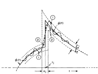
; p(r) z-, r large . (3)In fact, expression (1) defines a double sequence of function with regard to the para-meters r and N. Figure VIII-20 shows the function (1) respectively for: N =
20, r = 1, 2, 3, 4 and r = 4, N = 10, 20. The main spike has a height equal to N/2 p(r). The width of the main spike plays a basic role in our theories. A convenient measure of the width is provided by the so-called "triangular aperture", denoted by a(t) and given by
a(t) = 2 r) (4)
This aperture will be identified with aj, when they all are equal. The following
alter-native form of the window function has a fundamental importance in the constructive aspect of the theorem. It can be shown, by using elementary operations, that (1) is a trigonometric sum of order Nr - 1. That is, it can be written as
X=Nr-1
Scjp (t, r, N) N), = Pct r, A(rN) N ) cos Xt (5)
X-o
direct, but somewhat long, expansion of (1).
Numerical values of A(r, N), X will be
given for several selections of r and N.r = 2, N = 2 The following numbers, divided by 48, will give in the succession X = 0, 1, 2, 3 the coefficients A(2, 2), X
16, 23, 8, 1
r = 2, N = 5 The following numbers, divided by 750, will give A(2, 5), X in the
order X = 0, 1, 2, . .. , 9
250, 473, 404, 311, 212, 125, 64, 27, 8, 1
r = 2, N = 10 The following numbers, divided by 6000, will give A(2, 10), X in the
order X = 0, 1, 2, . .. , 19.
2000, 3943, 3784, 3541, 3232, 2815, 2488, 2089, 1696, 1327, 1000, 729, 512, 343, 216, 125, 64, 27, 8, 1
c5. The function 4(t) in tE(t a , tb) only, the corresponding sequence o-n(t) and the
window function Sc p are connected by an integral equation. Let us construct from (t) a periodic function (t), of period 2w, such that
p(t) (t); t (tt a tb) . (6)
The above mentioned integral is
+ T
c (t, r, N) = - (t + u) Scjp(u, r, N) du (7) -rr
where the index n has been momentarily omitted, but it will be restored later as n = Nr - 1. A simple heuristic reasoning reveals to us almost immediately the resemblance of o- (t, r, N) and p (t) and the monotonic approach of the first towards the second when the values of r and N are suitably selected. The conclusion follows directly by considering the spike shape and definitive passive character of Scjp. For suppose r and N are selected so that the "triangular aperture" a(t) = 2,r p(r)/(N/2) is much smaller than the subinterval of more rapid continuous fluctuation of p (t). Since the window function Sc j(u) is almost zero outside the aperture interval -at/2 < u < +at/2 and since
P
(t) changes slowly in the above aperture interval it follows thatat /2 +
o" (t, r, N)= p(t) SCjp (u) du (t) )du = P(t)
-a
at/2
-w+ rr
1 =
i
Scjp(u, r, N) du--for all positive integer values of r and N.
c
6.
We will discuss now, with some technical detail, the mode of approach
of a-n(t) towards
#p(t)
when the Scjp(t) is used as kernel.
The general trend of convergence follows the general lines of Fig. VIII-19. The
aperture aj
=
a(t
)= 27(p(r))/(N/2).
Let us consider the convergence in a k neighborhood. It can be shown that the
magnitude hk of the steps over the (t) and partial jumps from one step k to the next
are respectively given to a very high degree of approximation.
*
B(r 1 1)
hk =+ r Srp(r)(
S(2k +
2 2r3))
hk
(r
2
+
1
- p(r)n(2k
+1)
2r k = 1, 2,(9)
where: +, and - signs correspond respectively to the lower and upper part of
and after the jump of q(t). B(r + 1/2, 1/2) is the complete Beta function. The continuous approach curves when measured from the above mentioned upper parts are given by
C2(k) =
'p(r) w(2k + 1)
C 1(k)
= hk- C2kh
where: the + and - signs correspond as above. I I
B (x)(r + , 1) is the incomplete Beta function of variable argument x =
c(t) before
lower and
(10)
(cos
22)
p
is an auxiliary step variable as it is indicated in Fig. VIII-21;
-
<
I<
+
,
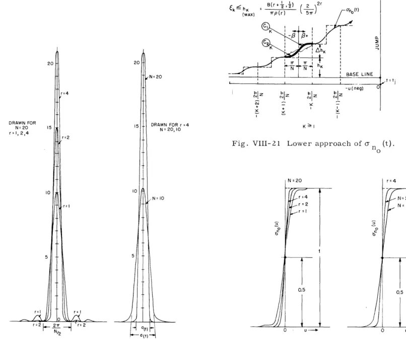
The graph and construction of the functions C2(k) and C (k) is illustrated in Fig. VIII-21,
where only the lower part of (n(t) before the jump is shown. For mere convenience,
Equations (9) and (10) refer to the vicinity of a normalized jump equal to 1.
B x)(r +,
the curves C2(k) and Cl(k) are measured over a horizontal line instead of the curved (t) and the reader must make mentally the correction for the curved line he has in mind.
We will now show that the set of tolerances -k fixes immediately the parameter r. For each jump the maximum deviation hk corresponds to k = 1. Then, for a jump of
c(t
+) - (t -) one must have1 1
B(r + ) Z_2r
ak
<[?(tj
+ )- (tj- (11)T
p(r)
5
/
Therefore, if
a
and J are respectively the largest k and largest jump of c(t) in t E (ta, tb), then the required value of r is a solution of the equation.1 1
SB(r 2' , 2 2r 2 2(r- 1) 1
J X (1)
T p(r)
57
p(r) (r)! (r -1)!
(5r)The second member decreases rapidly as r increases. For example, for r = 1, 2, 3, this member attains respectively the values 0. 127 . . , 0. 000148 . . , 0. 00000243 . . . consequently, we can specify very small tolerances, even when we use the first few integer values of r. The heights of the successive steps are now computed by means of the formula (11). They attain extremely small values for K large. The above results
confirm that the vertical scale used in Fig. VIII-19 has been greatly exaggerated.
Let us consider now the convergence behavior in an a. aperture. In the a. neighbor-hoods, the function cr (t) rises from around '(tj-) to c(t. +); the smaller the aperture a., the better the imitation of the original jump. In certain engineering problems it
is required that the above aperture must be very small. We will explain how the second index N can be fixed by the selection of the aperture. We may proceed as follows.
First, select an adequate at and estimate, or compute, the "modulus of oscillation" w(at) of the function cj (t) inside ak neighborhoods only. The term modulus of oscillation is to be understood here as it is defined in current books of analysis. It can be shown that
w(at)
must never exceed the smallest k. The condition can be satisfied with ease by simply selecting an at smaller than the subinterval of largest fluctuation of $P(t) (not containing the point of discontinuity).Second, take the largest aj, and set max. aj = a(t). Since the index r has already
been fixed, then the second index N is given by
N =2T
X 2 p(r)
(13)
Let us introduce the notation n0 = Nr - 1. The exact expression of no (t) inside our
approximation is obtained as follows. Consider a jump of size
p(t.+)
-p(t
-) = J which occurs at the point t.. Let t -- t. = u. Then, for relatively larger values of N and r one gets the simple expressionoa (t)
no 1 2 1 J. 2Z + Z+ ; -1<Z<1J
2u N(t - tj) a(t) a(t) Z a - < u < + (14) t 2 r p(r)It can be shown that the steepest tangent of a n (t) occurs at t = t. and has exactly the value
d
(o0W
a(t)• = 2 (15)
t=tj
Equation (14) shows that at a point of discontinuity o no(t) converges, for all values of r and N, towards J /2. Consequently, the values of pl' p2 and Co are respectively 1, 1, 0 (for the particular Scjp(t) window function). Figure VIII-22 shows how the func-tion r no(t) behaves at the vicinity of a normalized jump (one unit height), for different values of N and r. It is almost impossible to draw the deviation of 0-n (t) and
'p(t)
out-side the at neighborhood because its magnitude is very small.c 7 . In the last subsection c6, we have indicated how to find the values of r, N and
the corresponding simple expression (approximate) of ono(t) respectively in a k and a. neighborhood. In this subsection, we will explain how to construct (exactly) the set of no sinusoidal waves, whose sum produces no (t), as it is stated by the theorem. The procedure is simple. First, take P (t) and, by using well-known methods, find the first no = Nr - 1 Fourier coefficients. Let us use the notation
2 + h cost + h2 cos 2t + .. + h cos n t+
(t) =
o
+ gl sint + g2 sin 2t + . .. + gn sinnot +.. (16)
or the alternate form
p(t) = + K1 sin(t + K) +.
.+
Kn sin(nt + K (17)where the first (2n 0 + 1) coefficients are now supposed to be known. It can be shown that
R r=4
10
Fig. VIII-21
Fig. VIII-20 The Jackson-LaValle Poussin kernel.
titj
K I
Lower approach of o n (t).
0
U
---Fig. VIII-22 Behavior of convergence towards
the normalized jump when the Sc p window is used.
Z-I
X=no
0=nono(t)
= (t r, N) d(r, N),X cos X t + e(r, N),X sin tX=o
X=l
X=n 0>
C(r, N), X sin
(t
+K
X)(18)
X=owhere
d = h A(r, N), X(r, N), X
X
p(r)
A
e
(r,
N), X
e(r, N), X g p(r) C(r, N = h + g Ar, N),X (18')(r,
N),X pr)18)The coefficients
A(r, N),
. are obtained directly from the window function expansion,
as it was explained in the subsection c
4.
Equations (18) and (18') represent the
con-structive process which is indicated by part II of the general theorems.
c
8.
Summability. The reader has undoubtedly noted that the function
-
n (t) was
extracted from a sequence of (16) by a simple process of linear transformation. Let
us denote, in general, by
sn
the sum of the first n terms of the Fourier series expansion
of
(t) and by
crn(t),
the
corresponding transformed set according to (18). It
can be
shown that
cr
(t) is "N6rlund sum or mean" of s n(t).
In terms of the ordinary notation
the "NSrlund mean" is defined as follows.
Let [s
be a sequence.
Let lim s
= s
n
-w
(in our problem s exists and it is equal to
4 P(t)).
Let us associate to
[Sn]
the sequence
of positive real numbers
[pn
and introduce the notation
Pm
=PO
+P
+'
+P
m
P
for n,<
m
qm, n0
" n
> m
(19)
From the sequences [Sn]
and
[Pn]
we extract a new sequence, say a-
m, defined by the
ao
qo
.
O
0
0...
0
s
1
1,o
q1,
10...
O0
-
m, o qm, 1 m, 2 ' m, m (20)If the "weighting constants" p 0 p l,' . are such that p /Pm 0 for n fixed and m-co,
then it is said that the sequence [oa-n is the "N6rlund regular mean" of [sn].
It can be
shown that this is the case in our particular example (with Scjp(t) window function).
The weighting coefficients are given by
p
0PO
=2A
=2 A(r, n), 0
-A
(r,n), 1
Pg=
A(r, n), g - A(r, n)g+1
(21)
and Pm= p(r) for all values of r, N.
The positive character of p
0p l
etc. is guaranteed by the property
pr)=_2A >A
>A
>..>A1
(22)
p(r) = A(r, N), 0 >A(r, N), 1 >A(r, N), 2 >... >A(r,N), (rN-1) 2r-1
(2r - 1)! N
Besides the window function Sc p(t), we have also developed a group of windows which
correspond to other types of summability. For example, we know with detail the kernels
for (C, k), (A, 2), (VP) and Borel and Euler processes.
In this report there is not space
to discuss this matter.
c
9.
We will now occupy our attention with the network synthesis aspect of the theorem.
The Laplace transforms of (18) lead immediately to
X=n
(t)
=-n(t)
+
C(r, N), X
sZ +
Sk= i aX + s
where = tan K (23)
The corresponding transfer function for the unit step excitation is therefore:
=no
s(s + a )
C
0+
C(r, N), X
2
(24)
=l
aX
++
which, of course, is realizable with nondissipative passive elements. Expression (23)
itself is the corresponding transfer function for the unit impulse excitation.
which is not necessarily connected with the theorem, is the selective signal action of
such functions. We will explain this effect in regard to the Sc p window.
Suppose we intentionally fail to satisfy the first condition of page 67. That is, we
set the index N in such a way that the corresponding aperture a(t
)is now large in
com-parison with subinterval of rapid continuous oscillation of (t). For example, take
c(t)
= E
°sin vt and v such that Zrr/v < at.
Under this circumstance the corresponding
function crno(t) suffers a strong attenuation and also, for certain other classes of (t),
a considerable distortion with respect to (t). In the particular case of a sinusoidal
wave, as it was given above, it can be shown that
S, 0 for v integer > Nr - 1
cr no
(t )=
l
(-
k:I °
1
)m
2v
sin 6 Tr
A
rp(r)
6
=Osin
A(r, N), X
E sin v t (24)when v > Nr - 1. Here v = m + 6; m = largest integer contained in v. For a numerical
illustration, let us take r = 2, N = 5, Nr - 1 = 9, v= 10. 5.
The output wave has an
amplitude equal to an (t) = 0. 0001575 E
0sin(10. 5) t.
o
The above numerical result shows the drastic signal attenuation of the corresponding
networks for that type of function. In our general theories of signal separation, the
above selective properties of window functions play an important role.
d.
A CONCLUDING.REMARK ON THE GENERAL THEOREM
The above illustrative example, developed with Scjp(t) window function, will suggest
to the reader the trend along which the general theorem is conducted. The reader will
have no difficulty in extending the above ideas to a somewhat restricted, but still very
important, theorem. The proposed restrictions are imposed on the convergence
requirements (1) to (4).
Suppose, here that instead of specifying convergence conditions
on the reproduction of a certain arbitrary function, we will now be satisfied about the
mode of convergence, etc. in the vicinity of a rising part of a square pulse of ir duration.
Let o (t) now represent this response. cr (t) is supposed to be known and satisfies the
requisites imposed by the specific problem in question. As before, let u = t - t.. The
required window function is here equal to d/du
a
(u)
=
r '(u).
When a-'(u) is determined, then the first step is to expand o '(u) as a trigonometric
sum, of an appropriate finite order, by means of a well-known process of trigonometrical
interpolation.
The resulting approximate function is not, in general, capable enough to
represent o- '(u) inside tight tolerances. The second step consequently is to introduce a
linear transformation, by means of an auxiliary window function, such that the
trans-formed representation of - '(u), imitates very accurately the behavior of 0' '(u). The
third step is to introduce an integral representation of a (t), similar to the one given
by Eq. (7), and extract from it again the sequence r n(t) as a new finite trigonometric sum, which satisfies the convergence requirements imposed on o-(t). The Jackson-Poussin kernel is a very convenient kernel to settle this question,
The reader may have a more precise idea of the above procedure, if we illustrate the method of expansion when the Jackson-Poussin kernel is selected as basic window function, as it is suggested above.
Let us denote by Sc(u) the needed window function, which must produce a convergence behavior very similar to the window '(t).
First. The function Sc(u) is expressed as a finite linear combination of Jackson-Poussin kernels.
Sc(u)
xyE
qV
z
q Scjp
[(u +
), r, (N +
'y
(26)
(V=0 V=O where m = positive integer =v integer to be determined. 6 = shift parameter q = weighting "
For r relatively large, practically for r >, 2, the determination of the above parameters is rather simple, if one is satisfied with a solution which has the same rate of approach as the required one.
Second. Suppose that the term corresponding to v = o represents the dominant mono-tonic behavior in the reproduction of jump of the pulse. We set immediately 60 = o
yo
= o. The parameters r and N are determined as indicated in the example alreadygiven in other subsections. However, a small modification may be required: r must be large enough as to produce negligibly lateral deviation, much smaller than . For strategic reasons, we will keep this r the same in every component window. The constant N is now determined by the required aperture accepted as formation time of the pulse jump. Let us call this basic aperture ao(t) = 4w p(r)/N. On account of the selection of r each window component is reduced to its main spike.
Third. Determination of m. This number is equal to the total number of Ak sub-intervals, outside the main aperture ao(t), in which the rate of approach, now not necessarily monotonic, is specified. See Fig. VIII-19.
Fourth. Determination of yV. To each interval A we make correspond a Jackson-Poussin window component. This window possesses an aperture equal to the A ,. Con-sequently, a
v(t)
= 47r p(r) /(N + Yv) Av from which y is found as the closest integerwhich satisfies the above condition. If one sets, for example, a)
>o(t),
then is zero or negative.Fifth. Determination of 6 . The spike of each window function is centered over its A . Hence, 6 is equal to the distance from the origin u = o to the middle point of a .
v
Sixth. Determination of qv. It can be shown that the contribution of each term of (1) to the pulse formation is equal to q . This follows from the basic property
TF
Sc
[(u
u + ) r, (N + du 1 . (27)- T
Consequently, if the maximum deviation tolerance happens, for example, to be placed at l' then clearly
q =
The remaining q's are given by the rate of convergence numbers, which are indicated in Fig. VIII-19. For the normalized jump:
q v=h -h; h = o
Seventh. The above procedure determines completely the window Sc(u). Let y be the largest positive of the numbers y . It follows at once that : "Sc(u) is equal to a finite trigonometric sum of order (N + y) r - 1. " The property follows because every com-ponent of (1) is a trigonometric sum of finite order. By choosing av(t) > ao(t) then the
order is now rN - 1. The last result places the evidence on the important property: "It is possible to change the mode of approach towards c(t) and still keep the same number of trigonometrical components."
Eighth. The function o-no (t); no = (N + y) r - 1, which approaches p(t), as it is desired, is also a "trigonometric sum of order n ". The coefficients are found directly by carrying out the simple integral
+-r
Sn (t) P (t + u) Sc (u) du (28)
--in which ~ (t) is expended as a Fourier series.
Ninth. The window function (26) may represent "monotonic" as well as "oscillatory" or "mixed" approach. The method yields all the required constants equally well.
The above explanation sounds simple in principle. However, this process involves delicate steps and technicalities which cannot be presented in this short report.