Communication in a Poisson field of interferers

Communication in a Poisson Field of Interferers

by

Pedro C. Pinto

Licenciatura, Electrical and Computer Engineering

Oporto University (2003)

Submitted to the Department of Electrical Engineering and Computer Science

in partial fulfillment of the requirements for the degree of

Master of Science in Electrical Engineering

at the

MASSACHUSETTS INSTITUTE OF TECHNOLOGY

September 2006

©

Massachusetts Institute of Technology 2006. All rights reserved.

Author

...

Department of Electrical Engineering and Computer Science

September 11, 2006

Certified by ...

...

Moe Z. Win

Associate Professor

Thesis Supervisor

Accepted by ...

...

...

.. .. . '

,

...

Arth r C. Smith

MASSACHUSET S ~r....-; I Chairman, Department Committee on Graduate Students

OF TECHNOLO(.

APR

3 0 2007

ARICHIVS

LIBRARIES

Communication in a Poisson Field of Interferers

by

Pedro C. Pinto

Submitted to the Department of Electrical Engineering and Computer Science

on September 11, 2006, in partial fulfillment of the requirements for the degree of

Master of Science in Electrical Engineering

Abstract

This thesis presents a mathematical model for communication subject to both

interfer-ence and noise. We introduce a realistic framework where the interferers are spatially

scattered according to a Poisson field, and are operating asynchronously in a wireless

environment; subject to path loss, shadowing, and multipath fading. We consider both

cases of slow and fast-varying interferer positions. Under this scenario, we determine the

statistical distribution of the cumulative interference at the output of a linear receiver,

located anywhere in the two-dimensional plane. We characterize the error probability

and capacity of the link, when subject to both network interference and thermal noise.

We derive the power spectral density (PSD) of the cumulative interference at any

loca-tion in the plane. We put forth the concept of spectral outage probability (SOP), a new

characterization of the cumulative interference generated by communicating nodes in

a wireless network. Lastly, we quantify the cumulative interference distribution, error

probability, channel capacity, PSD, and SOP as a function of various important system

parameters, such as the signal-to-noise ratio (SNR), interference-to-noise ratio (INR),

path loss exponent of the channel, and spatial density of the interferers.

The proposed model is valid for any linear modulation scheme (e.g., M-ary phase shift

keying or M-ary quadrature amplitude modulation), and captures all the essential

phys-ical parameters that affect network interference. Nevertheless, it is simple enough to

enable a tractable analysis and provide fundamental insights that may be of value to

the network designer. Finally, this work generalizes the conventional analysis of linear

detection in the presence of additive white Gaussian noise (AWGN) and fast fading,

allowing the traditional results to be extended to include the effect of interference.

Thesis Supervisor: Moe Z. Win

Acknowledgments

Many individuals have contributed to the success of this thesis. I am deeply grateful

to my advisor., Professor Moe Win, whose genuine support, enthusiasm, and advice

have been invaluable over the past two years, in both professional and personal terms.

Not only has he provided guidance through the intricacies of research, but he has also

helped in broadening my mind as a scientist and an individual.

I am indebted to Professor Alan Oppenheim for his counsel and mentoring since my

arrival to MIT. His advice has enabled me to better understand life and work at MIT,

and easily overcome all the difficulties that incoming students face.

I am thankful to Professor Marco Chiani and Professor Andrea Giorgetti at the

University of Bologna, for invaluable discussions on relevant metrics for characterization

of wireless systems; careful reading of the thesis manuscript; and advice on the extension

of the results to ultrawideband communications.

I thank L. A. Shepp, L. Greenstein, J. H. Winters, and G. J. Foschini, for insightful

comments regarding Poisson fields, outage metrics, spectral coexistence, and

multi-antenna systems.

I also thank my colleagues in the Wireless Communications Group at LIDS, for their

wise advice about the inner workings of MIT and LIDS, over the past two years.

Most importantly, I am greatly indebted to my family, for their unwavering

encour-agement to pursue my interests, and limitless support in all facets of life.

This research was supported, in part, by the Portuguese Science and Technology

Foundation under grant SFRH-BD-17388-2004, the Charles Stark Draper Laboratory

Robust Distributed Sensor Networks Program, the Office of Naval Research Young

In-vestigator Award N00014-03-1-0489, and the National Science Foundation under Grant

ANI-0335256.

Contents

1 Introduction

1.1 Interference Modeling .

...

1.2 Thesis Objectives and Organization .

...

1.3

Review of Stable Distributions .

...

2 System Model

2.1

Spatial Distribution of the Nodes .

...

2.2 Transmission Characteristics of the Nodes .

...

2.3 Propagation Characteristics of the Medium .

...

3 Representation and Distribution of the Interference

3.1

Complex Baseband Representation of the Interference

3.2 P-conditioned Interference Distribution . . . .

3.3 Unconditional Interference Distribution . . . .

3.4 Discussion .

...

. .

4 Error Probability

4.1

Slow-varying Interferer Positions

P

4.2 Fast-varying Interferer Positions P

4.3 Discussion ...

..

...

4.4 Plots

...

5 Channel Capacity

5.1

Capacity Outage Probability .

31

. . . .

.

31

.. . . .

.

34

.. . .

.

35

.. . . . .

.

36

39

. . . . .

. . . .

.

39

. . . .

. . . .

.

42

.

.

.

. . .. .. .

44

.

. . ..

.

. . . .. .. .

4 5

5.2 Plots ...

6 Spectral Characterization of the Interference 59

6.1 Power Spectral Density of the Interference ... . . . .... . .... 60

6.2 Spectral Outage Probability ... ... . 62

6.3 Discussion ... ... ... 64

6.4 Plots .. . . ... . . . ... 64

6.5 Generalizations ... ... .. 65 7 Conclusions and Future Research 69 A Derivation of the Interference Representation in (3.9)-(3.12) 71 B Derivation of Vx in (3.16) 75 C Derivation of the Distribution of Y in (3.17) 77 D Derivation of the Distribution of A in (3.20) 79

List of Figures

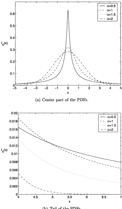
1.1 _{Stable densities for varying characteristic exponents a (/3 = 0, -y = 1,}

p =-:0) ... . ... ... ... . . ... . ... 21

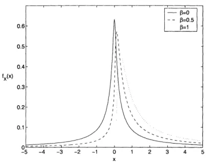
1.2 Stable densities for varying skewness parameters P (a = 0.5, / = 1, # = 0). 22 1.3 Stable densities for varying dispersion parameters y (a = 1,

3

2.2 Asynchronism between different transmitting nodes. In the observation interval [0, T], a change in constellation symbol of node i occurs at ran-dom time t = Di, from Vf-e jOi to VE-ej °i. The distribution of Di is

assumed to be U(0,T) ...

. .

.

.

...

28

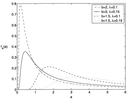
3.1 P.d..f. of A for different amplitude loss exponents b and interferer densities A. 38 4.1 Typical decision region associated with symbol sl. In general, for a

constellation with signal points sk = ISklek and k = I, l k=1.. . four parameters are required to compute the error probability: Ok,l and

"k.l

(as depicted); Bk is the set consisting of the indices for the signal points that share a decision boundary with Sk (in the example, B1 = {2,3,4});

and Wk,l = (k + 1 -2

Ck/cos((k

. . .

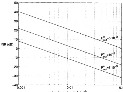
, =-: 10dB, p* = 10-2). ... ... .. 46 4.3 Error outage probability plots for a heterogeneous network (where SNR

4.4 Error outage probability plots for a homogeneous network (where SNR = INR) and slow-varying interferer positions P. ... ... . . . ... 49 4.5 Average error probability plots for a heterogeneous network (where SNR /

INR in general) and fast-varying interferer positions P ... . ... 50 4.6 Average error probability plots for a homogeneous network (where SNR =

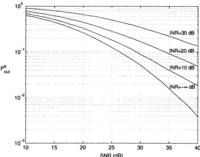
INR) and fast-varying interferer positions P. ... ... ... .... ... 51 5.1 Channel model for capacity analysis. .... ... ... ... 55 5.2 Capacity outage probability Put versus the SNR of the probe link, for

various interferer-to-noise ratios INR (R = 1 bit/complex symbol, A = 0.01 m-2

b=2, ro=1m, a, = 10dB) ... . ... ... ... 57

5.3 Capacity outage probability Put versus the transmission rate R, for var-ious interferer spatial densities A in m-2 _{(SNR = INR = 20dB, b = 2,}

ro = 1m, as = 10dB) ... .. . .. ... .. 58

6.1 Effect of the transmitted baseband pulse shape p(t) on the PSD and the outage probability PSout(f) (P = 10dBm, T = 10-6 s, A = 0.1m -2_{, b = 2,}

a = 10dB) ... ... 66 6.2 Effect of the spectral mask shape rm(f) on the outage probability PoSut(f)

(square p(t), P = 10 dBm, T = 10-6 s, A = 0.1m -2_{, b = 2, a, = 10dB). 67}

6.3 Spectral outage probability Post(f ) versus frequency, for various

trans-mitted powers P (square p(t), T = 10-6 s, A = 0.1 m- 2, b = 2, as = 10 dB,

m(f) = -60dBm/Hz). ... ... .. .. . 68

6.4 Spectral outage probability Put(f) evaluated at f = 0, for various inter-ferer spatial densities A in m- 2 _{(square p(t), T = 10}- 6 _{s, b = 2, as = 10 dB,}

List of Tables

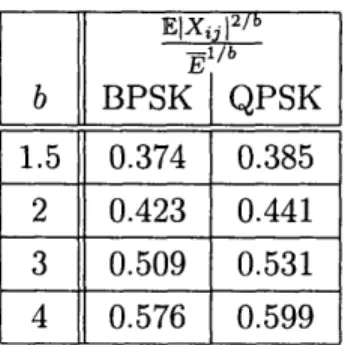
2.1 Typical signal amplitude loss exponents b for various environments. . 29 3.1 EIIX 3j12/b for various amplitude loss exponents b and modulations. Note

that for M-PSK modulations, this quantity is proportional to /b, where

Abbreviations

AWGN

additive white Gaussian noise

c.d.f.

cumulative distribution function

CS

circularly symmetric

FCC

Federal Communications Commission

GPS

Global Positioning System

i.i.d.

independent identically distributed

INR

interference-to-noise ratio

IQ

in-phase/quadrature

M-PAM

M-ary pulse amplitude modulation

M-QAM

M-ary quadrature amplitude modulation

p.d.f.

probability density function

PSD

power spectral density

r.v.

random variable

SNR

signal-to-noise ratio

SOP

spectral outage probability

Notation

IP{A}

probability of event A; also IPA {A}

E{X}

expected value of random variable X; also Ex{X} and X

EJX

(

E{(Xji}

V{X }

variance of random variable X

I(X; Y)

mutual information between random variables X and Y

X

-

the

distribution of the real random variable X

X -

the

distribution of the complex random variable

X

X NI

the distribution of random variable

X

conditional on

Y

U(a, b)

uniform distribution in the interval [a, b]

Exp(A)

exponential distribution with mean 1/A

Af(p, g2) real Gaussian distribution with mean ,/ and variance a2

A/(O,

a2)

circularly symmetric complex Gaussian distribution, where the real and

imaginary parts are independent, identically distributed

K(0,

S(a, , 'y) real stable distribution with characteristic exponent a, skewness 0,

disper-sion -y, and location u = 0

S,(a, 0, y) circularly symmetric complex stable distribution, where the real and

imag-inary

parts are independent, identically distributed S(a, 3, -y)

fx (x) probability density function of random variable X

Fx(x) cumulative distribution function of random variable X exp(x) ex

log2(x) base 2 logarithm

In(x) natural logarithm sign(x) signum function

Q(x)

Gaussian

Q

function; Q(x) =

• f

e- -dt

F(x) Gamma function;

F(x)

Ei(x) Exponential integral function; Ei(x) = -

f

IIx(t)ll

L2 norm of x(t);

IIx(t)II

=

vi

x(t)

_dt

Y{x(t)} Fourier transform of x(t) ]R real numbers

C complex numbers

j

x* complex conjugate of x Re{x} real part of x

Im{x} imaginary part of x I identity matrix

Chapter 1

Introduction

1.1

Interference Modeling

In a wireless network composed of many spatially scattered nodes, there are two funda-mental impairments that constrain the communication between nodes: thermal noise and network self-interference. Thermal noise is introduced by the receiver electronics

and is usually modeled as AWGN, which constitutes a good approximation in most cases. Self-interference, on the other hand, is due to other transmitter nodes, whose radiated signals affect receiver nodes of the same network. For simplicity, interference is typically approximated by AWGN with some given power [1, 2]. However, this ele-mentary model does not capture the physical parameters that affect self-interference, namely: 1) the spatial distribution of nodes in the network; 2) the transmission charac-teristics of nodes, such as modulation, power, and synchronization; and 3) the propaga-tion characteristics of the medium, such as path loss, shadowing, and multipath fading. If, instead, we use a Poisson point process to model the user positions, then all these parameters are easily accounted for, and appear explicitly in the resulting performance expressions.

The application of the Poisson field model to cellular networks was first investigated in [3] and later advanced in [4]. However, the authors either ignore random propaga-tion effects (such as shadowing and multipath fading), or restrict the analysis to error

probability in non-coherent FSK modulations. In other related work [5], it is assumed that the different interferers are synchronized at the symbol or slot level, which is typi-cally unrealistic. In [6,71, the authors choose a different approach and restrict the node locations to a disk or ring in the two-dimensional plane. Although this ensures the number of interferers is finite, it complicates the analysis and does not provide useful insights into the interference problem. Lastly, none of the mentioned studies attempts a spectral characterization of the interference, focusing instead on other performance metrics.

1.2

Thesis Objectives and Organization

The main research contributions of this thesis are as follows:

* We introduce a realistic framework where the interferers are spatially scattered according to an infinite Poisson field, and are operating asynchronously in a wire-less environment subject to path loss, log-normal shadowing, and fast fading. Our analysis is valid for any linear modulation scheme, and easily accounts for all the essential physical parameters that affect network interference, which appear explicitly in the resulting performance expressions.

* We specifically address two different scenarios: one where the interfering nodes are slow-moving, and another where they are fast-moving.

* We determine the statistical distribution of the cumulative interference at the output of a linear receiver, located anywhere in the two-dimensional plane. * We characterize the error performance of the link (in terms of average and outage

probabilities) when subject to both interference and thermal noise, for any linear modulation scheme.

* We analyze and provide expressions for the capacity of the link, when subject to both network self-interference and thermal noise.

* We derive the power spectral density (PSD) of the cumulative interference at any location in the two-dimensional plane, for any linear modulation scheme.

* We put forth the concept of spectral outage probability (SOP), a new charac-terization of the cumulative interference generated by communicating nodes in a wireless network.

* We quantify the cumulative interference distribution, error performance, channel capacity, PSD, and SOP as a function of various important system parameters, such as the signal-to-noise ratio (SNR), interference-to-noise ratio (INR), path loss exponent, and spatial density of the interferers. Our analysis clearly shows how the system performance depends on these parameters, thereby providing insights that may be of value to the network designer.

The thesis is organized as follows. Chapter 1 presents the scope and contributions of the thesis, and briefly reviews stable distributions. Chapter 2 describes the system model. Chapter 3 derives the baseband representation and distribution of the cumula-tive interference. Chapter 4 analyzes the error performance of the system. Chapter 5 analyzes the channel capacity. Chapter 6 characterizes the spectrum of the cumula-tive interference and introduces the concept of spectral outage probability. Chapter 7

concludes the thesis and suggests directions for future research.

1.3

Review of Stable Distributions

In the framework proposed in this thesis, stable distributions play an important role in the modelling of interference. Stable laws are a direct generalization of Gaussian distributions, and include other densities with heavier (algebraic) tails. They share many properties with Gaussian distributions, namely the stability property and the generalized central limit theorem [8, 9].

E{ejwX} has the form [81

xexp [-wyJwj (1 - jp sign(w) tan 2) + jw~ _{] , a 1,}

exp [-yIwl (1 + j- sign(w) In w) +

jw

A real stable distribution can therefore be characterized by four parameters:

a E (0, 2] Characteristic exponent, which controls the heaviness of the p.d.f. tail. If

a = 2, then X - Af(p, 2-y).

p E [-1, 1] Skewness parameter. The cases where 0 < 0, = 0, 13 > 0 correspond to0 a p.d.f. which is skewed to the left, symmetric around the center p, and skewed to the right, respectively.

y E [0, oc) Dispersion parameter, which behaves like the variance. p E I

R

We use X - S(a, 0l, 7, p) to denote that r.v. X has a real stable distribution with

parameters a,

/3,

Figures 1.1 to 1.3 depict stable p.d.f.'s for various parameters a, 0, and y.

Some useful properties of stable r.v.'s which are used in this thesis are provided below.

Property 1.1 (Scaling Property). Let X - S(a,

/,

kX - S(a, sign(k)P, lklay).

Property 1.2 (Decomposition Property). Let X - S(a, 0,

y).

X

=

v/VG,

1Unless otherwise indicated, in this thesis we only deal with distributions where p = 0, and therefore use the simplified notation X - S(a, 0, -y).

fx(X)

(a) Center part of the PDFs.

fx(x)

4 4.! b b.b b t.bI

X

(b) Tail of the PDFs.

fx(x)

Figure 1.2: Stable densities for varying skewness parameters 0 (oz = 0.5, y = 1, u = 0).

fx(x)

-5 -4 -3 -2 -1 0 1 2 3 4 5

x

where V S (, 1, cos

!)

A more detailed treatment of stables distributions, including its definitions and

properties, can be found in [8-11].

Chapter 2

System Model

2.1

Spatial Distribution of the Nodes

In the proposed model, we account for the spatial distribution of users by assuming an infinite number of nodes distributed according to a homogeneous Poisson point process in the two-dimensional plane. Typically, the terminal positions are unknown to the

network designer a priori, so we may as well treat them as completely random and use a Poisson point process.

A two-dimensional homogeneous Poisson point process is characterized by the fol-lowing properties (121:

1. If N(17) denotes the number of nodes located inside a region R of the plane, then the r.v.'s N(Ri) are independent if the regions Ri are non-overlapping.

2. Given that a node is inside region R, its position is uniformly distributed in that region.

3. The probability P{k in R} of k nodes being inside region R depends only on the area A.R of the region (not on its shape or location in the plane), and follows a Poisson distribution given by

0 Probe transmitter node

0 Probe receiver node

* Interfering node

--- I

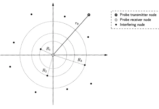
Figure 2.1: Poisson field model for the spatial distribution of nodes. where A is the (constant) spatial density of nodes, in nodes per unit area.

The Poisson point process can then be described by the single parameter A, which we use to denote the spatial density of interfering nodes. We define the interfering nodes to be all terminals which are transmitting within the frequency band of interest, during the time interval of interest (e.g., a symbol or packet time), and hence are effectively contributing to the interference. Then, irrespective of the network topology (e.g., point-to-point or broadcast) or multiple-access technique (e.g., time or frequency hopping), the proposed model depends only on the density A of interfering nodes.' In what follows, we will use interchangeably the terms node, interferer, user and terminal to mean interfering node.

The proposed spatial model is depicted in Fig. 2.1. For analytical purposes, we assume there is a probe link composed of two probe nodes: one receiver node, located at the origin, and one transmitter node (node i = 0), deterministically located at a distance ro from the origin.2 All the other nodes (i = 1... oo) are interfering nodes,

1_{Time and frequency hopping can be easily accommodated in this model, using the splitting} prop-erty of Poisson processes to obtain the effective density of nodes that conitribute to the interference.

2

whose random distances to the origin are denoted by

{Ri}',

•

Our goal is then to determine the effect of the interfering nodes on the probe link.

2.2

Transmission Characteristics of the Nodes

To account for the transmission characteristics of users, we consider that all interfering nodes employ the same linear modulation scheme, such as M-ary phase shift keying

(M-PSK) or FM-ary quadrature amplitude modulation (M-QAM). Furthermore, they

all transmit at the same power P - a plausible constraint when power control is too complex to implement (e.g., decentralized ad-hoc networks). For generality, however, we allow the probe transmitter to employ an arbitrary linear modulation and arbitrary power P0, not necessarily equal to those used by the interfering nodes.

The case where the probe and interfering nodes use a different modulation and power may c-orrespond to an heterogeneous scenario with a large number of identical secondary users (e.g., cognitive-radio terminals) interfering on a primary link. The case where the probe and interfering nodes use the same modulation and power, on the other hand, may correspond to a sensor network scenario, where there is a large number of indistinguishable, spatially scattered nodes, with similar transmission characteristics.

In terms of synchronization, we consider an asynchronous system where different terminals are allowed to operate independently. As depicted in Fig. 2.2, node i trans-mits with a random delay Di relative to node 0, where Di - AU(O, T). Thus, node 0

initiates symbol transmissions at times nT by convention, while node i initiates symbol transmissions at times nT + Di. Note that to analyze the error probability and channel capacity, we only need to consider one symbol interval, 0 < t < T; to characterize the spectrum of interference, on the other hand, we need consider the waveforms over all

time, -oo < t < +oo.

Lastly, in terms of demodulation, the probe receiver3 _{employs a conventional linear}

detector. Typically, parameters such as the spatial density of interferers and the

prop-stochastic quantities.

3

~AAIf

.JH

1

H4#

IAAAAAAAAAAAA

VIjeji

Vre~'

e

~~±JJ±±JJ0

fJ0rgf\%o

Figure 2.2: Asynchronism between different transmitting nodes. In the observation interval [0, T], a change in constellation symbol of node i occurs at random time t = Di, from vE-eej i to V/Eeejo. The distribution of Di is assumed to be 11(0, T).

agation characteristics of the medium (e.g., shadowing and path loss parameters) are unknown to the receiver. This lack of information about the interference, together with constraints on receiver complexity, justify the use of a simple linear detector, which is optimal in the presence of AWGN.

2.3

Propagation Characteristics of the Medium

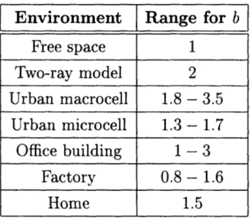
To account for the propagation characteristics of the environment, we assume a 1/rb median signal amplitude decay with distance r. The parameter b is environment-dependent, and can approximately range from 1 (e.g., hallways inside buildings) to 4 (e.g., dense urban environments).4 Table 2.1 gives typical values of b for different environments [13, 14]. The use of such decay law also ensures that interferers located far away from the origin have a negligible contribution to the total interference observed at that point, thus making the infinite-plane assumption reasonable.

'In this thesis, we will refer to b as the "amplitude loss exponent", which corresponds to a decay in

signal amplitude, not in signal power.

symbols:

node 0

symbols: node i

Environment

Range for b

Table 2.1: Typical signal amplitude loss exponents b for various environments. Experimental results show that the 1/rb deterministic propagation law is only the median behavior of the signal. Typically, a signal transmitted through a wireless chan-nel will experience random variation due to blockage from objects in the signal path (shadowing), and constructive-destructive addition of different multipath components (multipath fading). These two random effects are independent and multiplicative.

In this thesis, we use a log-normal model to capture the shadowing effect. Specifi-cally, the corresponding received signal strength S is log-normal distributed with p.d.f. given by

1 1 s

fs(s) = exp

In2

where Ip = K/rb is the median of S for some constant K, and a = as/2. The

parame-ter as, is the standard deviation of the instantaneous power, whose typical values range from 6 to 12 dB, depending on the environment [15, 161. In this model, the shadowing is responsible for random fluctuations in the signal level around the deterministic path loss K/rb. A useful fact is that a log-normal r.v. S with parameters y and a can be expressed as S =

jPe G,

Af(0,

The multipath effect is modeled as frequency-flat Rayleigh fading, which is superim-posed on the path-loss and shadowing of (2.1). Specifically, the Rayleigh fading affects the received signal by introducing a random phase 0 - U(0, 27r), as well as an amplitude

factor a which is Rayleigh distributed with p.d.f. given by

f·(a) =

exp

For normalization purposes, the parameter 3 is chosen such that the fading has unit power gain, i.e., E{a2} = 1.

We have thus a combined model for the path-loss, log-normal shadowing, and Rayleigh fading, where the overall effect of the channel propagation is captured by an amplitude factor rKb and a uniform phase q. The variations in the signal level

due to shadowing are usually slow, since they occur over distances that are proportional to the length of the obstruction object (typically, 10 - 100 m). On the other hand, the variations due to multipath fading are usually fast, occurring over distances on the order of the signal wavelength.

In the following chapters, we assume the shadowing and multipath fading are inde-pendent for different nodes i, and approximately constant during at least one symbol interval. Additionally, the probe receiver can perfectly estimate the shadowing and fading affecting its own link, hence ensuring that coherent demodulation of the desired signal is possible.

Chapter 3

Representation and Distribution of the

Interference

In this chapter, we characterize the cumulative interference measured at the origin of the two-dimensional plane, in terms of its probability distribution. Two distinct scenarios are considered: one where the interfering nodes are immobile or slow-moving, and the other where their positions change quickly with time. The resulting probability distributions will be used in later chapters to analyze the error probability and capacity of the probe link.

3.1

Complex Baseband Representation of the

Inter-ference

Under the system model described in Chapter 2, the cumulative signal Z(t) received by the probe node at the origin can be written as

Z(t) - a= e° \/2Eo cos(2rfct + Oo) + Y(t) + W(t), O < t < T, (3.1)

0

where the first right-hand term is the desired signal from the transmitter probe node,

Y(t) is the cumulative interference with

Rii

+ aieGi cos(2ft + O + )u(t - Di)) , 0 t < T, (3.2)

and W(t) is the AWGN with two-sided power spectral density No/2, and independent of Y(t).

The overall effect of the path loss, log-normal shadowing, and Rayleigh fading on node i is captured by the amplitude factor aie'Gi/Rb, where Gi -•- (0, 1), and by the uniform phase O5.1 The meaning of the remaining parameters is apparent from Fig. 2.2. We assume that r.v.'s ai, 0i, Gi, Di, E,, E', Oi, and 0' are statistically independent for different nodes i. In addition, each node transmits a sequence of i.i.d. symbols.

The probe node located at the origin receives and demodulates the cumulative signal Z(t), using a simple linear detector. This can be achieved by projecting Z(t) onto the orthonormal set { 1(t) =

-

By

Z =

foT

Z(t)

•j(t)dt,

j

= 1, 2, we can write

Zg =-Eo a- eGO- cos 80 + Yl + W1 (3.3)

2

=

_r-

+

where W1 and W2 are A/(0, No/2) and mutually independent. After some algebra

(Appendix A), Y, and Y2 can be expressed as

fT 0 eiX (3.5)

Y, = Y(t)Oj(t)dt =

(35)

Y2 TY( 2(t)dt =

(3.6)

1

Since we assume the probe receiver perfectly estimates the phase o0 of the multipath fading

where

Xil= ac

[-v§i

cos(9, +

0)

+

E

(1

-

)

cos(O' +

Oi)]

Xi

= ai [V

sin(6-i +i O) + /

(1 - D) sin(0( + O)] .

By defining the following complex quantities

Z = ZI + jZ 2

Y = Y + jY

W = W

+jW

Xi = Xil +

jXi

,

we can rewrite (3.3)-(3.8) in complex baseband notation as

=

te

V- oei

_{o + Y + W}

Se

X

eT

Di+

-

E

--'e

e3oj

and the distribution of W is given by

W

~

c

(0,

No).

(3.12)

Since different interferers i transmit asynchronously and independently, the r.v.'s {X }i%=1

are also independent.

In what follows, we derive the distribution of Y for two important cases: the

P-conditioned and unconditional cases. We will use P as a shorthand for "a

2_{Boldface letters are used to denote complex quantities.}

(3.7)

(3.8)

where

(3.9)

(3.10)

more succinctly, the "position of the interferers". The P-conditioned characterization

of Y is useful in scenarios where the interfering nodes are immobile or slow-moving.

The unconditional characterization, on the other hand, is relevant when the interferer

positions change quickly in time.

3.2

P-conditioned Interference Distribution

Consider, for example, a congested urban scenario where the interfering nodes are

spatially scattered. These nodes are subject to shadowing due to blockage from the

surrounding buildings and trees. Typically, the movement of the nodes during the

interval of interest (e.g., a symbol or packet time) is negligible. This has two

implica-tions: 1) the distances

{Ri}l=

of the interferers to the origin vary slowly; and 2) the

shadowing {Gi}Gl affecting those nodes also varies slowly, since the shadowing is

it-self associated with the movement of the nodes near large blocking objects. In this

quasi-static scenario, it is insightful to condition the interference analysis on a given

realization P of the distances {Ri}'=l and shadowing { Gi•

, of the interferers. This

will enable the derivation of the error outage probability of the probe link

-

a more

meaningful metric than the average error probability, in the case of slow-varying P

(17].

Because of its fast nature, the Rayleigh fading is averaged out in the analysis, no matter

whether we condition on P or not.

We now derive the P-conditioned distribution of the cumulative interference Y given

in (3.10)-(3.11). The work in

[181

shows that

Xi

in (3.11) can be well approximated by

a CS complex Gaussian r.v., such that

Xi - NVc(O, 2Vx),

Vx

V{Xij},

i > 1.

(3.13)

Then, conditioned on P, the interference Y =

=becomes

a sum of

indepen-dent CS Gaussian r.v.'s and is therefore a CS Gaussian r.v. given by

where A is defined as

0 2aG i

A = ₂ b . (3.15)

i=-1 i

Furthermore, after some algebra (Appendix B), Vx can be expressed as

= E{Ei} E{ jE cos(i - )}

(3.16)

Vx =

+

Z

6

I

1.

(3.16)

Because the r.v.'s {Xi}ý_

are i.i.d., Vx does not depend on i and is only a function

of the interferers' signal constellation. For the case of equiprobable symbols and a

constellation that is symmetric with respect to the origin of the IQ-plane

_{(e.g., M-PSK}

and M-QAM), the second right-hand term in (3.16) vanishes and

Vx

=

E/3, where

E

= E{Ei}, i

>

1 is the average symbol energy transmitted by each interfering node.

3.3

Unconditional Interference Distribution

The P-conditioned characterization of Y given in the previous section is useful when

the interfering nodes are immobile or slow-moving. However, it is sometimes more

use-ful to compute the distribution of the interference averaged over the user positions P.

Consider, for example, a sensor network (or any packet network) composed of many

scattered nodes with a short session life, i.e., each node periodically becomes active,

transmits a burst of symbols, and then turns off. Then, the set of interfering nodes

(i.e., the set of nodes that are transmitting and contributing to the interference) changes

often, and so do their distances {Rj}j__ and shadowing {Gj})j

. In this dynamic

sce-nario, it is insightful to average the interference analysis over all possible realizations

of user positions P.

We now derive the unconditional distribution of the cumulative interference Y given

in (3.10)-(3.11). It is known that sums of the form of (3.10), where the r.v.'s {Ri}

correspond to distances in a Poisson point-process and the

{Xij

have a CS distribution,

belong to the class of stable distributions

[8,

10], whose definition and properties were

respect _{to the origin if for every constellation}

briefly reviewed in Section 1.3. The complex r.v. Xi defined in (3.11) has in fact a CS distribution, since the phase q5 introduced by the Rayleigh fading is uniform in the interval [0,27r]. Then, Appendix C shows that the cumulative interference Y at the origin has a CS complex stable distribution given by

Y ,-c

(,S

A7C-

e2

/b

E X,,2/b

1--x

C =

x 1,(3.1)

cx

-

cos(nx/2)'

(3.18)

Both real and imaginary components of r.v. Y have real, symmetric, stable p.d.f.'s, similar to those shown in Figs. 1.1 and 1.3. Using (3.7)-(3.8), we can further express

E Xiyj2_{/b in (3.17) as}

EjXiyj2/b -

EaOi

+D

(-

+

T T,

=x(b)

=

(1i

where we have used the moment relation for the Rayleigh r.v.'s ai [191. Since different interferers i transmit asynchronously and independently, the parameter X(b) does not depend on i and is only a function of the amplitude loss exponent b and the interferers' signal constellation. Table 3.1 provides some numerical values for EIXijl2/b

3.4

Discussion

The results of this chapter have to be interpreted with care, because of the different

types of conditioning involved. In the unconditional case, we let P be random (i.e., we let {R••, be the random outcomes of an underlying Poisson point process, and {Gi•}__

pl/b

b

BPSK I QPSK

1.5

0.374

0.385

2

0.423

0.441

3

0.509

0.531

4

0.576

0.599

Table 3.1: EIXijl

_{/b for various amplitude loss exponents b and modulations. Note that}

for M-PSK modulations, this quantity is proportional to

/b, where E is the average

symbol energy transmitted by each interfering node.

be the random shadowing affecting each interferer). Then, the unconditional

interfer-ence Y is exactly stable-distributed and given by (3.17).

In the P-conditioned case, however, the positions of the interferers are fixed. Then,

A in (3.15) is also a fixed number, and the interference Y is approximately CS Gaussian

with total variance 2AVx, as given in (3.14). Note that since A in (3.15) depends on

the user positions P (i.e., {Ri)}z and {Gil"I), it can be seen as a r.v. whose value is

different for each realization of P. Furthermore, Appendix D shows that r.v. A has a

skewed stable distribution given by

(A

(3.20)

A

S a =

b,

PA

1,

where 0 < aA < 1 (or equivalently, b > 1) and C, is defined in (3.18). This distribution

is plotted in Fig. 3.1 for different b and A.

fA(a)

a

Chapter 4

Error Probability

In Chapter 3, we analyzed the distribution of the cumulative interference Y measured

at the origin. In this chapter, we build on those results and characterize the error

performance of the probe link, when subject to both interference and thermal noise.

We analyze both cases of slow and fast-varying interferer positions.

4.1

Slow-varying Interferer Positions P

As with the interference distribution, in the quasi-static scenario of slow-moving nodes

it is insightful to analyze the error probability conditioned on a given realization P of

the distances {Ril},

and shadowing {Gi •I, of the interferers, as well as on the

shad-owing Go of the probe transmitter node. We denote this conditional error probability

by Pe(Go, P).' Again, the fast Rayleigh fading is averaged out in the analysis.

To derive the error probability, we use the results of Section 3.2 for the P-conditioned

distribution of the cumulative interference Y. Specifically, using (3.12) and (3.14), the

cumulative received signal

Z

in (3.9) can be rewritten as

Z = V~eoaej• ° + W/', (4.1)

(X, Y) is used as a shorthand for

where

W'

=

00 2aG_i

A =

R

e

We have thus reduced the analysis to a Gaussian problem, where the combined noise W' is (approximately) Gaussian when conditioned on the location of the interferers. The corresponding error probability Pe(Go, 7) can be found by taking the well-known error probability expressions for detection of linear modulations in the presence of AWGN and fast fading [20-22], but using 2AVx + No instead of No for the total noise variance. Note that this substitution is valid for any linear modulation, allowing the traditional results to be extended to include the effect of interference.

In the general case where the probe transmitter employs an arbitrary signal constel-lation in the IQ-plane, the resulting symbol error probability conditioned on Go and P is given by M 1 t

Pe(Go, 7)

Z-Pk

2~

+

,l

dO

(4.4)

77A =

_rb(2AVx

(4.5)

is the received signal-to-interference-plus-noise ratio (SINR), averaged over the fast fading; M is the constellation size; {PkI}Fl are the symbol probabilities; Bk, k,1, Wk,1,

and /k,l are the parameters that describe the geometry of the constellation (see Fig. 4.1);

Eo = E{Eo} is the average symbol energy transmitted by probe node 0; A and Vx are

given in (3.15) and (3.16), respectively. When the probe transmitter employs M-PSK and M-QAM modulations with equiprobable symbols, (4.4) reduces to2

Pe(PSK(Go,-P)

=

A(

_{ir, sin}

1

2

(i))

_(4.6)

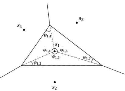
Figure 4.1: Typical decision region associated with symbol sl. In general, for a

con-stellation with signal points sk = Sk leJkk and (k = I 2, k = 1... M, four parameters

are required to compute the error probability:

and

are the angles that describe

the decision region corresponding to

(as depicted); Bk is the set consisting of the

indices for the signal points that share a decision boundary with

(in the example,

B

(

-2

pMQAMI(Go1P) = 4 1( 1 )

A(,

A(

where A(x, g) is given by

A(x, g) =

+

dO.

(4.8)

In the general expression given in (4.4)-(4.5), the network interference is accounted

for by the term 2AVx, where A depends on the interferer spatial distribution and

medium propagation characteristics, while Vx depends on the interferer transmission

characteristics. Since 2AVx simply adds to No, we conclude that the effect of the

in-terference on the error probability is simply to increase the noise level, a fact which is

intuitively satisfying. Furthermore, note that the modulation of the interfering nodes

affects the term Vx only, while the (possibly different) modulation of the probe

trans-mitter affects the type of error probability expression, leading to forms such as (4.6) or

In our quasi-static model, the conditional error probability in (4.4) is seen to be a function of the slow-varying user positions and shadowing (i.e., Go and 7). Since these quantities are random, the error probability itself is a r.v. Then, with some probability,

Go and P are such that the error probability of the probe link is above some threshold probability p*. The system is said to be in outage, and the error outage probability is

Pout = PGo,p(Pe(Go, P) > p*), (4.9)

In the case of slow-varying user positions, the error outage probability is a more mean-ingful metric than the error probability averaged over Go and P.

4.2

Fast-varying Interferer Positions P

The P-conditioned error probability given in the previous section is useful when the interfering nodes are immobile or slow-moving. However, there are cases (e.g., packet networks with short session life) where the set of interfering nodes changes often, and thus their distances {Ri} 1l and shadowing {Gj}=1 also change quickly with time. In

this dynamic scenario, it is insightful to average the error probability over all possi-ble realizations of interferer positions 7P. We denote this average error probability by

Pe(Go). Note that we choose not to average out the shadowing Go of the probe trans-mitter, since we have assumed the probe transmitter node is immobile at a deterministic distance ro from the origin, and thus Go is slow-varying.

To derive the error probability, we use the results of Section 3.3 for the unconditional distribution of the cumulative interference Y. Specifically, using the fact that any stable r.v. is conditionally Gaussian (i.e., Property 1.2), the cumulative interference Y in (3.17) can expressed as

Y = VK G, (4.10) where

G

-AN

=

2e2

/b

(ArO2EIXiI12/b)b,

i > 1,

(4.12)

with EIX lI,/b given in (3.19). Conditioning on r.v. B, we then use (3.12) and (4.10) to rewrite the cumulative received signal Z in (3.9) as

Z oe= a EGoejO-o + W',

where

W' =VBG + W

AKe

2BVG + No).

(4.13)

We have again reduced the analysis to a Gaussian problem, where the combined noise W' is a Gaussian r.v. Note that this result was derived without recurring to any approxi-mations - in particular, the Gaussian approximation of (3.13) was not needed here. We merely used the decomposition property of stable r.v.'s.

The corresponding error probability Pe(Go) can be found by taking the well-known error probability expressions for detection of linear modulations in the presence of AWGN and fast fading 120-22], using BVG + No/2 instead of No for the total noise variance, and then averaging over the r.v. B. Note that this procedure is valid for any linear modulation, allowing the traditional results to be extended to include the effect of interference.

In the general case where the probe transmitter employs an arbitrary signal con-stellation in the IQ-plane, the resulting symbol error probability conditioned on Go is given by

Pe(Go) =

k E

EB

+

M is the constellation size; {Pk}k=1 are the symbol probabilities; Bk, 7k,1, Wk,1, and

Eo = E{Eo} is the average symbol energy transmitted by probe node 0; B and VG are given in (4.11) and (4.12), respectively. When the probe transmitter employs M-PSK

and M-QAM modulations with equiprobable symbols, (4.4) reduces to3

PePSK (Go) = A(A17r, sin2 (i)) (4.16)

pMQAM(Go) = 4 "e 1 - A A 2-2(-1)o ,2(M-1) - 4 41 --,2 A 4 - l) (4.17)

where A(x, g) is given by

A

=

1

EB

1

+ %

)

dO.

(4.18)

A

Xog)

=

_sin2

In our dynamic model, the error probability in (4.14) is seen to be a function of the random shadowing Go of the probe link, and is therefore random. Then, with some probability, the slow-varying Go is such that the error probability of the probe link is above some threshold probability p*, leading to an outage. The corresponding outage probability can thus be defined as

pet = PGo(Pe(Go0

)

In the case of fast-varying user positions, both Pe(Go) and Poet are useful and insightful performance metrics.

4.3

Discussion

In this chapter, we have analyzed the error probability of the probe link when subject to both network self-interference and thermal noise, and considered two distinct cases which differ only in the mobility of the interferers: the static and the dynamic scenario. The results of Section 4.1 for the static case are approximate, because they rely on approximation of Xi by a Gaussian distribution, as shown in (3.13). On the other hand, the results of Section 4.2 for the dynamic case are exact, since were derived

3

without recurring to the Gaussian approximation.

In addition, note that an approximation to error probability Pe(Go) in (4.14) can be obtained by averaging Pe(Go, P) in (4.4) over the interferer positions 7, i.e., Pe(Go)

Ep {Pe(Go, :P)}. Again, this is not exact because the expression for Pe(Go, P) relies on

the Gaussian approximation, while that for Pe(Go) does not.

We now analyze the dependence of the error performance on the density A of inter-fering nodes, and the average symbol energy E transmitted by each interfering node. For that purpose, we use (4.4), although (4.14) would lead to similar conclusions. In (4.4), the error probability Pe(Go, P) implicitly depends on parameters A and E through the product AVx in the denominator. This is because the dispersion parameter /YA of the stable r.v. A depends on A according to (3.20), and Vx is proportional to E as in (3.16). The dependence on A can be made evident by using Property 1.1 to write

AVx = bA Vx, where A is a normalized version of A, independent of A. We thus

conclude that the interference term AVx is proportional to AbE, where b > 1 in the proposed model. Clearly, the error performance degrades faster with an increase in the

density of interferers than with an increase in their transmitted power.

The relation between E and A is illustrated in Fig. 4.2, which plots the pairs (A, INR =

E/No) that lead to a constant Poeut. Clearly, for a fixed error outage probability, there is a tradeoff between the density and energy of the interferers: if E (or, equivalently, the INR) increases, A must decrease, and vice-versa.

4.4

Plots

We now quantify the outage and error probabilities derived in this chapter for several scenarios, and illustrate the dependence of these probabilities on the various parame-ters involved, such as the signal-to-noise ratio SNR = Eo/No, the interference-to-noise ratio INR = E/No, amplitude loss exponent b, interferer density A, and link length ro0.

Figures 4.3 to 4.4 illustrate the scenario of slow-varying interferer positions P, where the adequate performance metric is the outage probability Peut given in (4.9). Two subcases are analyzed:

INR (dB

interferer density k (m- 2

Figure 4.2: INR - A curves of constant Peut (BPSK, SNR = 40 dB, b = 2, ro = 1 m,

as = 10 dB, p* = 10-2).

1. Heterogeneous network: The probe transmitter is allowed to use an arbitrary power Po, different from the common power of the interfering nodes P, and hence SNR Z INR in general. This scenario is useful when the goal is to evaluate the impact of a large number of identical secondary users (e.g., cognitive-radio termi-nals) on the performance of a primary link.

2. Homogeneous network: The probe transmitter and interfering nodes all use the same power, and thus SNR = INR. This may correspond to a sensor network scenario, where there is a large number of indistinguishable, spatially scattered nodes, with similar transmission characteristics. In such a case, the goal is to evaluate the impact of the cumulative network self-interference on the performance of each sensor node.

Figures 4.5 to 4.6 illustrate the scenario of fast-varying interferer positions P, where the insightful performance metrics are the error probability Pe(Go) given in (4.14), or the outage probability Plut given in (4.19). For simplicity, we choose to plot the former, with Go = 1 (no shadowing on the main link). As in the case of slow-varying P, we

also analyze the subcases of heterogeneous and homogeneous networks.

For simplicity, the plots assume that all terminals (i.e., the probe transmitter and

interfering nodes) use BPSK modulation. To evaluate the corresponding PFut and

Pe(Go), we resort to a hybrid approach where we employ the analytical results given

in (4.4)-(4.9) and (4.14)-(4.18), but perform a Monte Carlo simulation of all the stable

r.v.'s involved (i.e., A and B) according to [23]. As an alternative, numerical

inte-gration of those equations is also possible, although computationally more involved.

We emphasize that the error probability expressions derived in this chapter completely

replace the need for bit-level simulation of the system in order to compute the error

performance.

For the heterogeneous case depicted in Figs. 4.3 and 4.5, we conclude that Peut and

Pe(Go) deteriorate as A or INR increase, for a fixed SNR. This is expected because as the

interferers' density or transmitted energy increase, the cumulative interference at the

probe receiver becomes stronger. Note, however, that in the homogeneous case where

SNR =

INR, the error performance improves as we increase the common transmitted

power P of the nodes (or equivalently, the SNR), although the gains become marginally

small as P

--

oc (see Figs. 4.4(b) and 4.6(b)). This happens because in the

interference-limited regime where SNR

=

INR > 1, the noise term No in (4.4) and (4.14) becomes

irrelevant, and so the SNR in the numerator cancels with the INR in the denominator,

making the performance independent of the transmitted power P.

The effect of the amplitude loss exponent b on the error performance, on the other

hand, cannot be easily described. As illustrated in Figs. 4.4(a) and 4.6(a), an increase

in b may degrade or improve the performance, depending on the value of the link

length ro and other parameters. This is because b affects both the received signal of

interest and the cumulative interference in a non-trivial way

-

in the former through

the term 1/rg; and in the latter through oA and yA in (3.20), or through aB, YB, and

10 15 20 25 30 35 40 SNR (dB)

(a) Pot versus the SNR of the probe link, for various interference-to-noise ratios INR (BPSK, b =2, A = 0.01in- 2, ro= i, as = 10dB, p* = 10-2).

10

1 15 20 25

SNR (dB)

30 35 40

(b) Poet versus the SNR of the probe link, for various interferer spatial densities A in in- 2

(BPSK, INR = 10 dB, b = 2, ro = 1 in,

a = 10 dB, p* = 10-2).

Figure 4.3: Error outage probability plots for a heterogeneous network

INR in general) and slow-varying interferer positions P.

(where

SNR

5

...

...

I

1

I

I

IV

.

.

.

.

.

.

.

.

.

.

.

.

.

.

.

.

.

.

.

...

...