Publisher’s version / Version de l'éditeur:
Building Science, 2, 1, pp. 29-36, 1966-11-01
READ THESE TERMS AND CONDITIONS CAREFULLY BEFORE USING THIS WEBSITE.
https://nrc-publications.canada.ca/eng/copyright
Vous avez des questions? Nous pouvons vous aider. Pour communiquer directement avec un auteur, consultez la première page de la revue dans laquelle son article a été publié afin de trouver ses coordonnées. Si vous n’arrivez pas à les repérer, communiquez avec nous à [email protected].
Questions? Contact the NRC Publications Archive team at
[email protected]. If you wish to email the authors directly, please see the first page of the publication for their contact information.
NRC Publications Archive
Archives des publications du CNRC
This publication could be one of several versions: author’s original, accepted manuscript or the publisher’s version. / La version de cette publication peut être l’une des suivantes : la version prépublication de l’auteur, la version acceptée du manuscrit ou la version de l’éditeur.
Access and use of this website and the material on it are subject to the Terms and Conditions set forth at
Surface temperatures and heat fluxes for flat roofs
Hoglund, B. I.; Mitalas, G. P.; Stephenson, D. G.
https://publications-cnrc.canada.ca/fra/droits
L’accès à ce site Web et l’utilisation de son contenu sont assujettis aux conditions présentées dans le site LISEZ CES CONDITIONS ATTENTIVEMENT AVANT D’UTILISER CE SITE WEB.
NRC Publications Record / Notice d'Archives des publications de CNRC:
https://nrc-publications.canada.ca/eng/view/object/?id=dfbd372c-9233-49d1-aa71-3fc81db33232 https://publications-cnrc.canada.ca/fra/voir/objet/?id=dfbd372c-9233-49d1-aa71-3fc81db33232
Build. Sci. Vol. 2. pp. 29-36. Pergamon Press 1967. Printed in Great Britain. UDC 697.9.001
Surface Temperatures and Heat Fluxes for
Flat Roofs
D. G. STEPHENSON?
The results of calculated and measured surface temperatures and heat fluxes for a ventilated flat roof are conzpared and discussed. The thermal response factor method of calculating heat fluxes and temperatures gives values in good agreement with measured values when the sol-air temperature (evaluatedfrom several derived fornzulae) includes the effect of long-wave radiation exchange between the roof and sky.
1. INTRODUCTION
THE RANGE of temperatures that can occur within the walls and roof of a building must be known before these elements can be designed properly. The rate of heat transfer through the inner surface of the walls and roof must also be known in order that the heating and cooling loads may be determined. It is important, therefore, that a designer be able to calculate the temperatures and heat fluxes for any combination of materials exposed to any inside and outside conditions.
As every calculation procedure involves some assumptions, the accuracy of any method must ultimately be established by comparing the results
of calculations with experimental results. This
paper compares the results of calculations made at the Division of Building Research, National Research Council, Ottawa, with results obtained experimentally for a flat roof and calculated by an RC-network method at the Royal Institute of Technology, Division of Building Technology, Stockholm.
The non-steady, non-periodic heat flux through a new roof construction was calculated first using measured values of the temperatures at the inner and outer surfaces of a roof as data. The results were compared with the measured values of the heat flow at the inner surface. The calculations were then repeated using sol-air temperature (evaluated in various ways) and inside air temperature instead of surface temperatures. This latter case corresponds to the normal design heat loss calculation.
"Docent (Assoc. Prof.) Royal Institute of Technology, Stockholm, Sweden; Visiting Scientist, Building Services Section, Division of Building Research, National Research Council, Canada.
fResearch Officer, Building Services Section, Division of Building Research, National Research Council, Canada.
2. EXPERIMENTAL STUDY
2.1 Data used for calculations
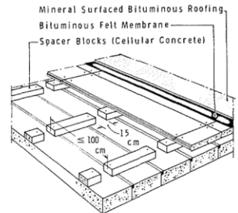
For the calculation of surface temperature and heat flux the roof (figure 1) was approximated by three homogeneous layers (figure 2):
1. 7.5 cm of cellular concrete (representing the top slab and the topping),
2. 7 cm dead air space (ventilation and spacer blocks ignored),
3. 20 cm of cellular concrete.
The moisture content of the cellular concrete was 6.5 per cent (by weight) for layer 1 and 5 per cent for layer 3.
M i n e r a l Surfaced B i t u m i n o u s Roofing B i l u m i n o u s Felt Membrane-,
1
rSpacer Blocks ( C e l l u l a r Concrete)I
I
Fig. I . Isometric figs1r.e of the flat roof constrrrction.
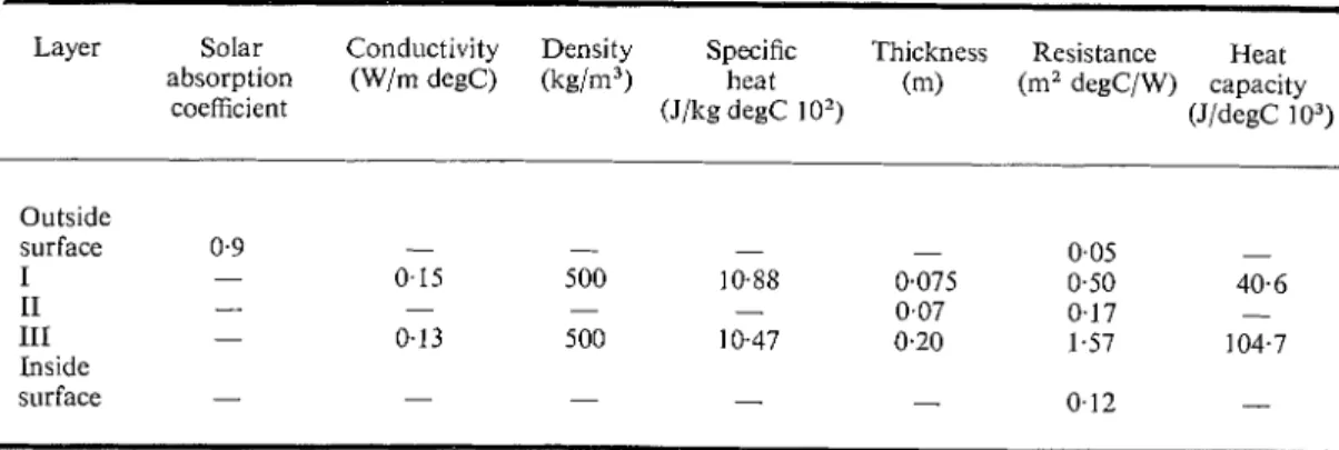
The thermal properties listed in Table 1 take account of these moisture contents, conductivity being based on the simple linear relationship[l]:'j
B. I. Hoglund, G. P. Mitalas and D. G. Stephenson
where
Table C- 1. Coeficiertts ard properties
Layer Solar absorption
coefficient
Conductivity (W/m degC)
Density Specific Thickness
(kg/m3) heat (m) (J/kg degC 1 02) Resistance Heat (mz degC/W) capacity (JIdegC 1 03) Outside surface I I1 I11 Inside surface
k,,i = thermal conductivity in the moist state, kcal/mh degC,
lc, = thermal conductivity in the dry state,
kcal/m h degC,
U = per cent moisture by weight, dry basis. The solar absorption coefficient, a, for black bituminous roofing is assumed to be 0.9; and the resistances at the outside and inside surfaces equal 0.05 and 0.12 m2 deg C/W, respectively.
... .,..a ... ....,. , " , . .< .: ...:.. ,. .
.:I
L a y e r I : 7 . 5 crn C e l l u l a r :: <., ...,.*' .,,..: .; :. .
. . . ,. .:. . . ,,;,;.,. .. ..I ... I . . ' , . . . >.. ...L C o n c r e t e!
L a y e r 11: 7 crn Air S p a c eFig. 2. Simplifie(1 corrstrrictiori rlividerl irlto tllree layers for t11e calcrrlatiorrs.
2.2 Measuremnents
Measurements were taken at different periods from December 1963 to April 1965[2].
Hentflo~i] through the roof system was measured
with thermo-electric heat flow meters at four points on the bottom, warm surface.
Temperature (air and surface) was measured by
means of copper-constantan thermocouples. These and the heat flow meters were connected to potentiometric recorders (Honeywell-Brown). The therrnocouples on the top of the roof were covered with the roof surfacing material.
So/ar racliation was measured by means of Kipp
and Zonen solarimeters.
Moisture content of the two cellular concrete
layers was determined at different times by removing cores.
2.3 Conclitions d~iritzg the period zrsec1,for conzpnrisotz Heat flows and surface temperatures were cal- culated for a period of seven days in April 1965. During this time the weather varied from colnpletely overcast to very clear conditions. The daily total solar radiation incident on a horizontal surface varied from 4 to 15 MJ/m2 and the outside air
temperature from - 12 to
+
13°C. There was nosnow on the roof at any time during the week. The inside air temperature was steady, ranging between
+23 and +24"C.
3. RESPONSE FACTOR METHOD FOR CALCULATING HEAT FLUX
The temperatures and heat fluxes at the surface of a roof are related by the response factor sets:
Q , = i - , . X - T . Y (2)
Qi
= T o . Y - T i . Zwhere (3)
Q = heat flux (heat flow towards inside is
positive),
T = temperature,
subscripts o and i refer to outside and inside surface respectively.
X , Y and Z are the three sets of response factors
that characterize the heat flow through the roof. All of these quantities are in time-series form, i.e. each symbol represents a set of values.
The response factor method of computing heat flux through an element of a building has been described by Mitalas and Stephenson[3, 41 in papers that also give a method for computing the factors for a multilayer element such as this roof. The response factor method is particularly well suited for these calculations because it does not require the assumption of periodic conditions, nor any complex analysis of the driving temperatures. It is necessary to know only the values of the driving temperatures at regular intervals.
The calculation of heat fluxes using this technique involves the multiplication of the driving tem- peratures by the appropriate response factors and the summation of a series of such products. A desk calculator may be used, but it is preferable to prepare a simple program to enable a digital computer to d o the arithmetic.
The method is applicable only to situations where the thermal conductivity and specific heat of the materials are independent of time. If the coeffi- cients of heat transfer a t the surfaces are constant, they can be combined with the roof response factors to give a set of over-all factors that relate surface fluxes to the outside and inside air temperatures. Table 2 gives the factors for the roof alone that must be used with roof surface temperatures.
Surface Temperatures and Heat Fluxes for Flat Roofs
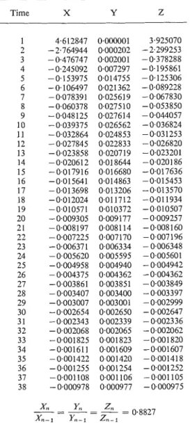
Table C-2. Surface to srrrface response factors for the pat roof
Time X Y Z
4. RESULTS OF CALCULATIONS
4.1 Heat $ow based on measured s~nmface
tet??peratures
The heat fluxes at both the inner and outer surfaces of the roof were calculated using the experimentally measured values of the roof surface temperatures. The calculated fluxes are shown in
Table 3, column 3, along with experimentally
measured values. The good agreement between calculated and measured values shows that the surface temperature and heat flux measurements are self-consistent, that the values chosen for thermal properties are appropriate, and that the air space ventilation and the spacer blocks have a negligible effect on the measured heat flux.
4.2 Mean heatfloul basecl on n7ean inside and outside
air fen7peratuws
The daily average heat flow is sometimes cal- culated by multiplying the average inside-to-outside air temperature difference by the over-all trans- mittance for a building element (Table 3, column 4). This simple method gives very large errors because it neglects solar radiation entirely. For the 7th and 8th of April (clear days) the average heat flow through the test roof calculated in this way is about 50 per cent higher than the average of the measured values. If the thermal resistance of the outer layer is discounted because the air space is vented, the discrepancy is even higher.
4.3 Heat $ 0 1 ~ baserl on simple sol-air tem??perahrres
The simplest expression for sol-air temperature first given by Mackay and Wright[5] is
oSA
=sort
+
aIRowhere (4)
OSA = sol-air temperature,
8," = outside air temperature,
a = absorptivity of surface for short-wave
radiation,
Table C-3. Measctred arrrl calcltlated heat flow, daily meat1 ~.alltes ( W/nz2)
Computed heat flow based on the temperature difference Difference per cent
Measured 0,;-Q,, Q;,,-Q,, Q;,,-Qs,l 0;"-Bsn B;a-Q~,, Q;,-B,, 91-90 9 2 - 9 ~ (13-90 94-90 95-cl0 96-(10
Time heat flow 90 90 90 40 90 90
90 (1 1 (1 z 93 94 9 5 9 6
Apr. 2 6.7 (7.8) 8.9 (6.8) (6.5) (7.4 ) (7.6) (4- 16) -i-33 (+ 2) (- 3) (+lo) (+ 13) 3 7.4 7.8 8.9 7.2 7.1 7.4 7.6 i - 5 - t 2 0 - 3 - 5 0 i- 3 4 7.3 7.7 7.3 7.2 6.9 7.5 7.7
+
5 0 - 2 - 6 + 3 4 - 5 5 6.2 6.3 6.8 5.6 5.1 6.5 6.6 i- 2 + I 0 -11 -17+
6+
6 6 6.2 6.2 7.4 5.0 4.8 5.9 6.0 0 4-19 -19 -23 - 5 - 3 7 6.0 6.0 9.1 5.8 5.7 6.3 6.4 0 $52 - 3 - 6 + 5 4 - 6 8 7.0 7.3 10.4 5.8 5.7 7.3 7.6 4 - 4 1 - 4 9 -17 -18 $ 4 i - 8 Notes:All days before 2 April are assumed to havc the same conditions as 2 April. q l , q3, q5 and q s are computed by means of the rcsponse factor method. q4 is conipi~ted by means of RC-network.
32 B. I. Hoglund, G. P. Mitalas and D. G. Stephenson
I = short-wave radiation incident on unit area
of roof,
R, = resistance to heat transfer at outside
surface.
The daily mean values of heat flow based on hourly values of OsA, obtained by both the response factor and an RC-network method, are shown in Table 3, columns 5 and 6, respectively; values of
0 , were calculated from measured values of O,, and
I, and an assumed average R, of 0.05 m2 deg C/W.
This average value of R, is in accordance with the
measurements of Brown[6].
The daily mean heat flows calculated by both
methods, using O,, are in good agreement with
each other, but agreement with measured values is not as satisfactory as was obtained with measured roof surface temperatures. A comparison of hourly values, given in figures 3 and 4 for cloudy and clear days, respectively, indicates a greater discrepancy for clear days.
Fig. 3. Measured and calclrlated heat flow for a clolrdy day (3 April), follo~vi~~g a day with fairly clolrdy conditioirs.
2 4 u I 3 2 1 0
Similarly, calculated outside surface temperatures
using OsA, were in reasonably good agreement with
measured values on a cloudy day and during daylight hours, but the measured temperatures on clear nights were lower than the calculated ones. In fact, the surface temperature falls well below the outside air temperature on clear nights. This indicates that O,, as given by equation (4) is too high, especially at night. Equation (4) is based on the assumption that the sky radiates as a black body at outside air temperature, but the results in Table 3 and figures 3 and 4 show that this is not valid. Mackay and Wright[5] recognized this fact but used the simple form for cooling calculations as this gave conservative results. In 1952 Mackay suggested a modified formula that included a term for long- wave radiation [discussion of reference 71.
-
-
-
9 rneas-
-0---.--
q 8,. - q o:,-
-0- 9 8:; - - - 1 1 1 1 1 1 / 1 1 1 1 ~4.4 Heat flow calculation based on mod$ed sol-air
temperature
8;,
0 4 8 1 2 16 2 0 2 4
A P R I L 3 T I M E
In Appendix A a modified sol-air temperature based on Brunt's[8] sky radiation formulae is given by:
1
where
H, = outside surface heat transfer coefficient,
a = solar radiation absorption factor,
I = solar radiation incident on the surface,
E = emissivity of the surface,
R = long-wave radiation incident on the
surface,
q = constant (in a linear approximation of the
aT4 curve),
hc = outside surface convection heat transfer
coefficient,
O,, = outside air dry-bulb temperature.
-
9 rneas-0- q 8,,
2
--.--
q o:,1
0 4 8 1 2 16 2 0 24
A P R I L 8 T I ME
Fig. 4. Meas~rrad and calclrlated heat flow for a very clear day (8 April), follo~vii~g n day wit11 clear corldiiio~~.
Calculations based on this sol-air temperature give good agreement for both heat flow and surface temperatures. As shown in Table 3, the biggest discrepancy between calculated and measured daily mean values of heat flow is only + 6 per cent. The calculated heat flow for each hour of the day is very close to that measured on both clear and cloudy days, as is shown in figures 3 and 4.
The comparison of calculated and measured values indicates that the modified sol-air tem-
perature
O
h
adequately accounts for both short-and long-wave exchange at the exterior surface. 4.5 Heat flow based on mnodiJied sol-air temperature
Ol.2
In Appendix B a modified sol-air temperature based on the equivalent radiant temperature of sky
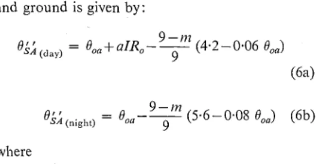
Surface Temperatures and Heat F/uxes for F/nt Roojs 3 3 and ground is given by:
where
M Z = sky clearness in oktas and all other symbols have same meaning as in equation (4). The last term in equation (6) takes account of the fact that the long-wave radiation from the sky is less than that from a black body at outside air tempera- ture.
The inside surface heat flux calculated using 0;;
is shown in Table 3 and in figures 3 and 4. Values are in good agreement with measurements and with values obtained with 0;, for all conditions
Fig. 5. The eqrrivaler~t radiarit temperatrrre of sky and ground
(OR) (effective re-radiatiorz temperature) as a furzction of the outside air dry-bulb tempe1.atur.e (O,,) during completely clear
nights, vertical and horizontal slrrfaces[6].
4.6 Time de/ay and decrement factor method Calculation of the actual heat flow for each time of day by the approximate ' time delay and decre- ment factor ' method for periodic heat flow as given in the I.H.V.E. Guide gives poor agreement with the measurements in this case, since the actual heat flow is non-periodic.
4.7 Some tlzermal clznracteristics of tlze roof The heat flow, as mentioned before, is determined on the under surface. During a 24-h period the maximum heat flow (at noon) can be about 40 per cent higher and the minimum (at midnight) about
30 per cent lower than the mean value. This
variation, on the other hand, is very small compared with the variation on the top surface, where the extreme values can be nine times lower or higher than the mean value.
The temperature fluctuation is effectively damped out by the roof construction. For example, the variation between maximum and minimum tem- perature on the outside surface can be more than 50 deg C, while it is only about 2 deg C on the inside surface.
Steady-state heat flow seldom occurs in the construction with such a high storage and the rapid fluctuations of air temperature, solar heating and radiation cooling. The temperature gradient is not linear, even for rather cloudy conditions, contrary to some common design assumptions.
The time lag is found to be 10-12 h ; the heat loss was maximum at about mid-day and minimum during the night.
5. CONCLUSION
Non-steady-state heat flow through a roof can be calculated quite accurately by the response factor method, even when the conditions are not periodic. It is necessary, however, that the sol-air temperature allow for the fact that clear sky emissivity isless than unity. Results based on two different sol-air tem- perature formulae are in equally good agreement with the measured values.
Even an RC-network is fairly well suited for such calculations, but it is more laborious (for non- periodic conditions) because of practical difficulties in producing the driving functions by function generators.
Calculation of the inside surface heat flux by the ' time delay and decrement factor ' method gives poor agreement with experimental results because the assumption of periodic conditions was not satisfied in the experimental situation.
The results confirm that the effect of free ventila- tion of the air space and the cold bridge effects of spacer blocks are negligible on the measured heat flux, and also confirm that the assumed properties are appropriate for this roof. The material above the air space has
a
significant effect on the heat loss through-the roof.Ackno~vledgement-This is a contribution from the Division of Building Research, National Research Council, Canada, and is published with the approval of the Director of the Division.
REFERENCES
1. A. ELMROTH and I. HOGLUND, Influence of moisture on the thermal resistance of external walls of cellular concrete-Relating to two newer types of construction.
RilernICIB Symposium, Moistrlre Problems in Buildings, Helsinki (1965).
2. A. ELMROTH and I. HOGLUND, Analys av varmeflode och temperatur-fordelning for
34 B. I. Hoglund, G. P. Mitalas and D. G. Stephenson
3. G. P. MITALAS and D. G. STEPHENSON, Room thermal response factors. To be presented at the ASHRAE Semi-Annual Meeting, Detroit, 30 January to 2 February (1967). 4. D. G. STEPHENSON and G. P. MITALAS, Cooling load calculations by the thermal
response factor method. To be presented at the ASHRAE Semi-Annual Meeting, Detroit, 30 January to 2 February (1967).
5. C. 0 . MACKAY and L. T. WRIGHT, Summer comfort factors as influenced by the thermal properties of building materials. ASHVE Trans. 49 (1943).
6. G. BROWN, Varmeovergang vid byggnaders ytterytor (Heat transfer at exterior surfaces of buildings). Transactiorzs Nat. Swedish Coun. Building Res., Stockholm, 27 (1956).
7. V. PARMELEE and W. W. AUBELE, Radiant energy emission of atmosphere and ground.
ASHVE Trans. 58 (1952).
8. D. BRUNT, Physical and Dynanzic Meteorology. University Press, Cambridge (1952).
9. 0 . ONGUNLESI, Solar radiation and thermal gradients in building units. Building Sci.
1, 1 (1965).
10. R. W. BLISS, Jr., Atmospheric radiation near the surface of the ground; A summary for engineers. Solar Energy 5 (3) (1961).
11. A. Angstrom, Beitr. Phys. frei Atnzos. 14, 1 (1928).
APPENDIX A
ModiJied sol-air tenzperature based on Brunt's sky radiation formulae
A heat balance for an outside horizontal surface
gives :
~ I + E R - E R ~ + ~ , ( B ~ ~ - B ~ ) = Q (A-1)
where
a = solar radiation absorption factor,
I = solar radiation incident on the surface,
E = emissivity of the surface,
R = long-wave radiation incident on the
surface,
eRs = long-wave radiation emitted by the sur- face,
h, = surface convection heat transfer coeffi- cient,
0, = surface temperature,
Boo = air dry-bulb temperature.
The heat flux Q can also be expressed using sol-
air temperature
Ho (B;,- 6s) =
Q
(A-2)where
Ho = surface heat transfer coefficient
B;, = sol-air temperature.
Elimination of Q in equations (A-1) and (A-2)
gives
1
B;, = - (al+ E R - eRs+hC Boa-h, Bs)+ 0,
Ho
(A-3)
The long-wave radiation incident on a horizontal surface is the radiation emitted by the sky. This emission is a function of the sky cloud conditions. Assuming that the form factor from a horizontal surface to the part of the sky that is cloudy is directly proportional to the sky clearness number
m (oktas)*, then
* m ranges from 0 to 8,
m = 0 denotes clear sky,
rn = 8 denotes completely overcast sky.
where
= average sky emissivity,
E , = clouded sky emissivity,
eCs = clear sky emissivity.
The emissivity of the clear sky is given in reference
[7] [see also reference 81
ecs = 0.55
+
0.33 2/(P,") (A-5)where
P,, = water vapour pressure at ground level,
inches mercury,
and the emissivity of the cloudy sky is 0.96[7]. Both emissivity values (i.e. cloudy and clear sky) are based on the assumption that the sky is at the ground level air dry-bulb temperature
therefore
R = en o T & (A-6)
where
To, = air dry-bulb absolute temperature,
o = Stefan-Boltzmann constant.
The black body emission can be approximated sufficiently accurately by a linear equation when the temperature undergoes moderate variation, i.e.
o T 4 % q + p e 04-71
where
p = slope of the o T 4 curve at B,,, i.e., p = 40 T,3,
8, = time average of the surface temperature,
q = o T:-40, o T: (A-8)
Substitution of the linear expression for Rs in equation (A-3) and collection of terms gives
1
eiA
=-
[aI+ E R - ~q+
Itc Boa-
(EP+
h,) Bs]+
0,Ho
The surface temperature, B,, is eliminated from
equation (A-9) by making H, = ep+h,,
i.e.
This is then a modified sol-air temperature to be used in equation (A-2) to calculate surface heat flux.
Sui:face Temperatures and Heat Fluxes for Flat Roofs 3 5
APPENDIX B
Mod$ed sol-air temperature based on the equivalent temperature of sky and ground
The net outgoing long-wave radiation from a surface can be given by
Q, = ue (T,4 -Ti). (B-1)
Writing this equation
Qr = hr (0s - 0,)
then
hr = cre (T,
+
TR).
(T:+
T i )-
4creT& 4creToaz,,, (B-2) whereQr = long-wave radiation heat flow,
cr = Stefan-Boltzmann's constant,
l = emissivity of the surface for long-wave radiation,
T, = absolute temperature of the surface,
TR = absolute equivalent radiant temperature
of sky and ground,
h, = outside surface radiation heat transfer coefficient,
T,,, = time average of T, and TR
Toa,,, = time average of absolute outside air dry- bulb temperature.
The heat balance at the roof surface can now be written [compare reference 91:
80s aI- 11, (eon - 0,) - (h,
+
11,) (e, - e0,) = - k-
xa
03-5) where
a = absorptivity of surface for short-wave
radiation,
I = intensity of short-wave solar radiation
incident on the surface,
I?, = outside convection heat transfer coefficient, k = thermal conductivity,
80s
- = temperature gradient at the surface,
ax
8, = the equivalent radiant temperature of sky and ground.
Using the sol-air temperature ;; 6' the heat balance can be expressed
a
0s (h,+
h,) (6;; - 0,) = ho (6;;-
0,) =-
k
-
ax (B-7) giving whereh, = outside heat transfer coefficient.
Brown161 has given 8, as a function of the air
temperature
eO,
from values observed in Stockholmduring completely cloudless nights (figure 5). An approximation gives for a horizontal surface:
for a vertical surface:
This is a reasonable approximation, especially when the deviation in the observed values is relatively great. Brown's measured values for horizontal surfaces are in good agreement with calculated ones[lO].
During the daytime the net heat loss from the ground to the sky is practically the same as it would be at night with the same atmospheric conditions of temperature and humidity[8].
Thus for clear conditions
where
-
hr-
0.4 during the night and-
0.3 during theh0 day for a horizontal surface.
For a sky of 172 oktas cloud the last term in equation
(B-10) is to be multiplied by the ratio (9-m)/9 following a proposal by Angstrom[ll].
Equation (B-10) can now be separated into two parts
(B- 1 1) where
R, = outside surface resistance
(B-12) (at night I is zero).
36 B. I. Hoglund, G. P. Mitalas and D. G. Stephenson
APPENDIX C 5. Heat capacity
Conversion factor's 1. Linear rneasure l m = 100 cm = 39.3701 in 2. Bulk density 1 kg/m3 = 0.06244 Ib/ft3 3. Temperature 'C = (OF-32)/1.8 OF = 1.8'C+32 4. Specific heat 1 J/kg degC = 0.2388
.
l o p 3 7. Thermal condzictivit y1 W/m degC = 0.5778 B.t.u./ft 11 degF
6.933 B.t.u. in/ft2 11 degF 8. Thermal resistance
1 m 2 degC/W = 5.678 ft' h degF1B.t.u. 9. Surface coeficient
B.t.u./lb degF 1 W/m2 degC = 0.1761 B.t.u./ft2 11 degF
Les rtsultats de calcul et de mesurage de temperature de surface ainsi que de flux thermiques sont revus et comparts. La mtthode de rtponse du coefficient thermique, appliqute pour le calcul des flux de chaleur et des temperatures donnent les valeurs Ctant en conformitt satisfaisante avec les valeurs mtsurtes, sous la condition toutefois, que la temptrature de solarisation (evalute suivant plusieurs formules dtrivtes) comprend les effets d'tchange de la radiation d'ondes longues entre le toit et le ciel. Die Ergebnisse der berechneten und gemessenen Flachentemperaturen und Warmes- tromungen fiir ein ventiliertes flaches Dach wurden verglichen und besprochen. Die Methode des thermischen Reaktionskoeffizienten fiir die Berechnung von Warmestro- mungen und Temperaturen ergibt Werte, die mit den gemessenen Werten gut iibereinstimmen, wenn die solare Temperatur (an Hand mehrerer abgeleiteter Formeln abgeschatzt) die Wirkung des Austausches der langwelligen Strahlung zwischen Dach und Himmel einschliefit.