Small-Signal Modelling for In-Depth Modal Analysis of an MTDC System

HAL Id: hal-01244019

https://hal-centralesupelec.archives-ouvertes.fr/hal-01244019

Submitted on 17 Dec 2015

HAL is a multi-disciplinary open access

archive for the deposit and dissemination of

sci-entific research documents, whether they are

pub-lished or not. The documents may come from

teaching and research institutions in France or

abroad, or from public or private research centers.

L’archive ouverte pluridisciplinaire HAL, est

destinée au dépôt et à la diffusion de documents

scientifiques de niveau recherche, publiés ou non,

émanant des établissements d’enseignement et de

recherche français ou étrangers, des laboratoires

publics ou privés.

Small-Signal Modelling for In-Depth Modal Analysis of

an MTDC System

Samy Akkari, Jing Dai, Marc Petit, Pierre Rault, Xavier Guillaud

To cite this version:

Samy Akkari, Jing Dai, Marc Petit, Pierre Rault, Xavier Guillaud. Small-Signal Modelling for

In-Depth Modal Analysis of an MTDC System. 2015 IEEE Electrical Power and Energy Conference

(EPEC), Oct 2015, London, Canada. �10.1109/EPEC.2015.7379955�. �hal-01244019�

Small-Signal Modelling for In-Depth Modal

Analysis of an MTDC System

S. Akkari, J. Dai, M. Petit

Group of Electrical Engineering Paris (GeePs) CentraleSup´elec, CNRS UMR 8507,

UPSud and UPMC Gif-sur-Yvette, France samy.akkari@centralesupelec.fr

P. Rault

X. Guillaud

Laboratory of Electrical Engineering and Power Electronics (L2EP Lille)

´

Ecole Centrale of Lille Lille, France

Abstract—In this paper, the state-space model of a VSC-MTDC system is derived from individual components and a modified PI section model for cables is proposed which considers both core and screen conductors as well as their coupling. A modal analysis performed on the complete system reveals the influence of each component on the system modes and permits the identification of a dominant DC voltage mode. This mode has proved to be largely affected by the energy storage level of the DC grid, and to be predominantly influenced by the voltage-droop parameters of the converters, meaning that the DC voltage dynamic of the MTDC system can be imposed thanks to a judicious choice of the voltage-droop parameters.

Index Terms—HVDC, modal analysis, MTDC, state-space model.

I. INTRODUCTION

The ever increasing offshore wind energy installed capacity is pushing coastal nations to develop the HVDC technology which is the only feasible solution to transiting large amount of bulk power over long distances. In fact, due to the large capacitance of shielded cables, the capacitive current of an HVAC cable becomes so significant that no power can be delivered above 75 km [1]. The proliferation of offshore wind farms will most probably give rise to several DC links located in the same geographical zone. DC reinforcements, extensions and AC zone interconnections may lead to a Multi-Terminal HVDC (MTDC) grid in the future. According to recent publications, the Voltage Source Converter (VSC) is currently the most appropriate and mature technology to interconnect the wind farms and the mainland grids [2]. However, several issues remain to be tackled before meshed HVDC grids become a reality, such as DC fault current extinction (DC breakers), power flow dispatch and DC voltage control. On this last topic, the master-slave control technique used to operate the existing HVDC links is not suitable for meshed HVDC grids [3]. The voltage-droop control technique, described in [4]–[6], seems to be the best solution to safely and efficiently controlling MTDC systems.

Classical small-signal stability analysis, used for modal analysis, is a powerful tool to acquire a better understanding of an MTDC system. This paper first presents the small-signal modeling of a VSC-HVDC converter and its state-space representation with a similar approach to the one in

[7]. The choice of a model for the DC cables is investigated as well. Then, by associating the multiple state-space models of individual components, the state-space representation of a 5-terminal MTDC system is obtained and studied. In particu-lar, a dominant mode which drives the DC voltage dynamics of the DC grid is identified and traced. The participation factor of each eigenvector is computed in order to study the sensitivity of this DC voltage mode with regards to the other elements of the MTDC system. This mode is linked to the energy storage level of the system and is largely influenced by the value of the voltage-droop parameter of the converters.

The paper is organized as follows. In Section II, the small-signal modeling of a VSC-HVDC converter is presented and the state-space representations of its elements are obtained. In Section III, the choice of the DC cable model is explained and the state-space representation of the 5-terminal HVDC grid is obtained. Finally, in Section IV, the modal analysis of the MTDC system is performed and the participation factor of each element on the system modes is analyzed.

II. STATE-SPACE MODELING OF AVSC-HVDC CONVERTER

This section aims at obtaining the state-space model of each part of a VSC-HVDC converter and combining them to generate the model of a full VSC-HVDC converter of the form:      d dtx = A.x + B.u y = C.x + D.u (1)

A. Control strategy of a VSC-HVDC converter

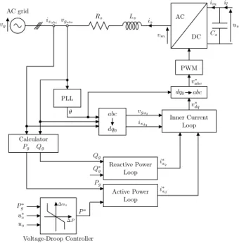
The global control of the VSC-HVDC converter is depicted in Figure 1. Some of the converters are equipped with a voltage-droop controller in order to participate in the DC voltage control. In fact, a converter equipped with a voltage-droop controller modifies its power reference according to the DC voltage by moving its operating point (P ,Udc) along the

characteristic line with a slope of _k1

v, where kv is the voltage-droop parameter. The converters connected to offshore wind farms are usually not equipped with a voltage-droop controller

since they inject into the DC grid all the available power regardless of the DC voltage.

vg AC grid Rs Ls is vm AC DC us Cs im il isabcvgabc PLL θ _abc dq0 Calculator Pg Qg Reactive Power Loop Qg Q∗ g i∗ sq Active Power Loop Pg i∗ sd P∗ P∗ g u∗ s us Voltage-Droop Controller ∆P ∆us Inner Current Loop vgdq isdq v∗ dq dq0 abc v∗ abc PWM

Fig. 1. Control Strategy of a VSC-HVDC converter.

B. Model of the physical system and the current-control loop The VSC-HVDC converter, modeled with its current control loop, is the base structure for any VSC model. As shown in Figure 1, the current control is carried out in the dq0 rotating frame. If the switching losses are neglected, the active power on the AC side of the converter matches the power on the DC side of the converter, i.e.

vmdisd+ vmqisq = usim (2) This non-linear equation is linearized by using the first order Taylor series. With each quantity composed of an operating point (denoted by the capital letter and the subscript 0) and a small variation (denoted by the Greek letter ∆), Equation (2) can be linearized as:

∆vmdIsd0+ ∆isdVmd0+ ∆vmqIsq0+ ∆isqVmq0= ∆usIm0+ ∆imUs0 (3)

The linearized current loop, the physical system on the AC side of the converter as well as the physical system on the DC side of the converter are depicted in Figure 2 (more details in [6], [8], [9]), where xid and xiq are the outputs of the integral part of the controllers corresponding respectively to the d-axis and q-axis projection of the dq0 frame.

From Figure 2, the state-space model of the current-controlled VSC is obtained, whose inputs are the current references in the dq0 frame, the DC voltage and the d-axis projection of the AC grid voltage, and whose outputs are the AC currents in the dq0 frame and the DC current.

C. Outer loop model

1) Active and reactive power loops: If the dq0 frame is chosen such that vgq = 0, the active power injected or extracted from the AC grid is:

pg= vgdisd (4)

where a positive pg corresponds to power extracted from

the DC grid and injected into the AC grid. The outer loop giving the d-axis current reference of a VSC is the active power controller potentially combined with a voltage-droop controller.

Equation (4) can be linearized as:

∆pg= ∆vgdIsd0+ ∆isdVgd0 (5) The block diagram of the active power loop is depicted in Figure 3, where xpis the output of the integral controller. For

more information about the feed-forward choice, see [10].

∆p∗ g ∆pg + − kip s Xp ++ feed-forward − ∆vgd Isd0 1 V_gd0 ∆i∗sd

Fig. 3. Linearized active power loop.

The state-space model of the active power loop can be obtained from Figure 3.

It is assumed that the q-axis current reference is provided by a reactive power controller. Since the reactive power loop has the same structure as the active power loop with the exception of a negative sign (since qg = −vgdisq), the reactive power loop state-space model is similar to that of the active power loop and is not further detailed here.

2) Voltage-droop controller: Some converters are also equipped with the voltage-droop controller [4], [11] depicted in Figure 4. This controller modifies the active power reference ∆p∗g of the active power loop of Figure 3.

This additional loop slightly alters the state-space model of the d-axis outer loop of the converter since it adds two additional inputs, ∆u∗_s and ∆u_s, such that the new active power reference ∆p∗_g

v of the active power loop obeys: ∆p∗_g

v = ∆pgv +

1 kv

(∆us− ∆u∗s) (6)

III. STATE-SPACE MODELING OF THE5-TERMINALHVDC GRID

A. DC cable model

Each DC line consists of two unipolar shielded cables (a positive and a negative pole), as shown in Figure 5, where cable screens are grounded at each end.

Initially, the DC cables were modeled by a classical PI equivalent, without taking into account the cable shields. However, replacing the classical PI equivalent model with the

∆i∗ sd ∆isd + − k_ii s xid kpi ++ + − + ∆vgd ∆vmd ∆isq ∆i∗sq + − k_ii s xiq kpi + + ++ + ∆vmq ∆vgq Lsω Lsω ∆vgd + + − Lsω 1 Rs+ Lss + − − ∆vgq Lsω 1 Rs+ Lss Is_d0 Vg_d0 Vg_q0 Is_q0 Σ ∆pm + − 1 Us0 ∆im Im0 ∆us ∆vmd ∆vmq ∆isd ∆isq

Fig. 2. Linearized model of the current-controlled VSC.

++ ∆p∗g ∆p∗gv + − −1 ∆us ∆u∗s Voltage Droop ∆p∗ v= 1 kv∆uv ∆uv ∆p∗v ∆pv ∆uv

Fig. 4. Linearized voltage-droop controller.

Fig. 5. DC lines layout.

more complicated but much more accurate wide-band model [12] noticeably impacts the DC voltage dynamics. This is illustrated in Figure 6, where the DC cable model’s impacts on the DC voltage dynamics are compared in EMTP-RV. It appears that the classical PI equivalent model produces undesirable oscillations, which do not exist with the wide-band model.

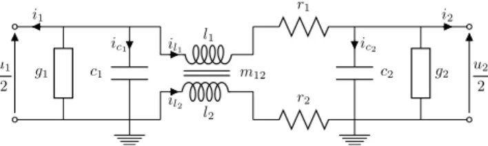
In-depth investigations revealed that the current flowing through the screen conductor is actually an important source of damping of the DC voltage. Therefore, a modified PI section model including both core and screen conductors as well as their coupling (modeled by a mutual inductance between these two conductors, as depicted in Figure 7 for the positive pole of the DC cable), have to be considered in order to acquire a more accurate model of the DC cable yet much simpler than the wide-band model.

Figure 6 shows that the response of this new model (called coupled PI equivalent model) is very close to the wide-band model reference. This validates the use of this DC cable model.

0 0.05 0.1 0.15 0.2 0.25 0.3 0.35 0.4 0.7 0.8 0.9 1 Time [s] DC V oltage [p .u .] Classical PI PI coupled Wide-band

Fig. 6. EMTP-RV simulation showing the impact of a power decrease on the DC voltage dynamics of different DC cable models.

m12 l1 l2 r1 r2 c1 c2 g1 g2 u1 2 u2 2 i1 i2 ic1 il1 ic2 il2

Fig. 7. Positive pole of the PI core-screen coupled model.

According to Figure 7, the Kirchhoff current law gives: ic1 = −i1− il1− g1

u1

2 ic2 = −i2+ il1− g2 u2

2 the Kirchhoff voltage law gives:

ul1 = u1

2 −

u2

2 − r1il1 ul2= −r2il2

and the evolution of the inductance currents and capacitor voltages obeys: duc1 dt = 1 c1 ic1 duc2 dt = 1 c2 ic2 Φ1= l1il1+ m12il2 Φ2= l2il2+ m12il1 ul1 = dΦ1 dt = l1 dil1 dt + m12 dil2 dt ul2 = dΦ2 dt = l2 dil2 dt + m12 dil1 dt

which yields: dil1 dt = l2ul1 l1l2− m212 − m12ul2 l1l2− m212 (7) dil2 dt = l1ul2 l1l2− m212 − m12ul1 l1l2− m212 (8) These equations give the state-space model of a DC line where the output voltage of Figure 7 is simply multiplied by 2 since each pole has the same length and the same characteristics.

B. 5-Terminal HVDC grid model

The studied system is a 5-terminal HVDC grid intercon-necting two offshore wind farms and three asynchronous AC grids as depicted in Figure 8. The parameters of the MTDC system are listed in Appendix.

vg2 ac dc Conv 2 vg3 ac dc Conv 3 Conv 5 dc ac Conv 4 dc ac ac dc vg1 Conv 1 l1 l2 l3 l6 l4 l5

Fig. 8. Topology of the HVDC grid.

Converters 1, 2 and 3 are equipped with voltage-droop controllers whereas converters 4 and 5 are equipped with regular active-power loops since they are connected to offshore farms and inject all the power harvested by the wind-farms into the DC grid. The initial power operating point of each VSC-HVDC converter as well as their voltage-droop coefficients1 are shown in Table I.

TABLE I

POWER REFERENCE VALUES AND VOLTAGE-DROOP COEFFICIENTS OF THE

VSC-HVDCCONVERTERS

Converter 1 2 3 4 5

Pg∗(MW) 200 200 -50 -162 -200

kv(p.u.) -0.4834 -0.4834 -0.4834 -∞ -∞

The global state-space model of the full MTDC system is obtained by summing the cable and station capacitors at the connection nodes and by combining the multiple state-space models [14], as shown in Figure 9. The final state-space model of the complete MTDC system consists of a 60x1 input vector, a 42x1 output vector, a 47x1 state vector, a 47x47 A matrix, a 47x60 B matrix, a 42x47 C matrix and a 42x60 D matrix.

1_{The voltage-droop parameter values were computed to achieve a time}

response of 100 ms, see [13] for more information.

Active Power Loop + Voltage Droop

Reactive Power Loop

Current Loop + Physical System ∆i∗ sd1 ∆i∗ sq1 ∆p∗ g1 ∆u∗ s1 ∆vgd1 ∆q∗ g1 ∆isd1 ∆isq1 ∆im1

Active Power Loop + Voltage Droop

Reactive Power Loop

Current Loop + Physical System ∆i∗ sd2 ∆i∗ sq2 ∆p∗ g2 ∆u∗ s2 ∆vgd2 ∆q∗ g2 ∆isd2 ∆isq2 ∆im2

Active Power Loop + Voltage Droop

Reactive Power Loop

Current Loop + Physical System ∆i∗ sd3 ∆i∗ sq3 ∆p∗ g3 ∆u∗ s3 ∆vgd3 ∆q∗ g3 ∆isd3 ∆isq3 ∆im3

Active Power Loop

Reactive Power Loop

Current Loop + Physical System ∆i∗ sd4 ∆i∗ sq4 ∆p∗ g4 ∆vgd4 ∆q∗ g4 ∆isd4 ∆isq4 ∆im4

Active Power Loop

Reactive Power Loop

Current Loop + Physical System ∆i∗ sd5 ∆i∗ sq5 ∆p∗ g5 ∆vgd5 ∆q∗ g5 ∆isd5 ∆isq5 ∆im5 HVDC Grid ∆us1 ∆us2 ∆us3 ∆us4 ∆us5 FULL MTDC SYSTEM

Fig. 9. System association scheme used for the state-space representation of the 5-terminal MTDC system.

IV. MODALANALYSIS OF THE5-TERMINALHVDC GRID A modal analysis can now be performed on the final state-space model of the 5-terminal HVDC grid presented in Figure 8. Table II summarizes its eigenvalues and indicates the rela-tive participation of the state variables to the different modes (corresponding to their respective eigenvalues), quantified by the state variables participation factors [15].

The 47 modes (size of the state vector) are divided into two distinct groups. The first group is associated to the DC grid (λdc1,...,16) while the second group corresponds to those associated to the VSCs (λc1,...,31):

• Modes associated to the eigenvalues from λdc1 to λdc8 are mostly affected by the elements of the DC grid but are also influenced by the parameters of the active power loops (state variable xp) of the three converters equipped

with a voltage-droop controller.

• Modes associated to the eigenvalues from λdc9 to λdc16 depend on the topology of the HVDC grid and are exclusively affected by the elements of the DC cables. These modes can be identified in the state-matrix of the HVDC grid alone (without the converters).

• Modes associated to the eigenvalues from λc1 to λc14 correspond to those inner current loops (state variable xiq for the q-axis, xid for the d-axis) of the converters whose outer loops (state variable xq for the reactive power loop,

TABLE II

MODALANALYSIS OF THE5-TERMINALHVDC GRID

Eigenvalues Freq._(Hz) Damp._ratio Dominant states

λdc1,2 −56.7 ± j1028 164 0.055 xp1, xp2, xp3,

λdc2,3 −56.9 ± j995 158 0.057 ∆us1, ∆us2, ∆us3

λdc5,6 −57.1 ± j724 115 0.079 ∆us4, ∆us5

λdc7,8 −57.7 ± j635 101 0.090

il₁₁, il₂₁, il₁₄,

il₂₄, il₁₅, il₂₅,

∆us1, ∆us2, ∆us3, ∆us4, ∆us5

λdc9,10 −117.1 – – il11, il21, il12, λdc11,12 −4.47 – – il₂₂, il₁₃, il₂₃, λdc13 −4.45 – – il₁₄, il₂₄, il₁₅, λdc14 −4.49 – – il₁₄, il₂₄, il₁₅, DC Grid λdc15,16 −0.604 – – il25, il16, il26, λc1...14 −195.2 ± j230 37 0.650 xq1...5, xi_q1...5, xp4, xp5, xi_d4, xi_d5 λc15...18 −193.8 ± j226 36 0.650 ∆us1, ∆us2, ∆us3, ∆us4, ∆us5,

xi_d1, xi_d2, xi_d3, λc19,20 −184.0 ± j238 38 0.611 xi_d4, xi_d5, il₁₁, il₂₁, il₁₂, il₂₂, il₁₃, il₂₃, λc21 −22.6 – – il₁₄, il₂₄, il₁₅, il₁₄, il₂₄, il₁₅, il₂₅, il₁₆, il₂₆ λc22 −28.8 – – ∆is_d1...3 Con v erters λc23...31 −29.7 – – ∆is_d1...5, ∆is_q1...5

behavior of the MTDC system. In fact, the reactive power loops of all five converters, as well as the active power loops of converters 4 and 5, are independent of the MTDC system since their output remains invariably constant. As anticipated, the eigenvalues of these modes correspond to the dynamics of the inner current loops (tuned for a response time of 15ms).

• Contrary to the eigenvalues from λc1 to λc14, modes associated to the eigenvalues from λc15 to λc20 corre-spond to the inner current loops (d and q-axis) of the three converters whose active power loops are highly impacted by the behavior of the MTDC system through the DC voltage droop. In particular, the modes associated to the conjugate eigenvalue pair λc19and λc20 correspond to complex interactions between the voltage-droop con-trollers of converters 1 to 3, the converters’ inner current loops and the DC grid. Those two modes describe the dynamic of the DC current in the whole MTDC system. While the eigenvalues λc15 to λc18 coincide with the dynamics of the inner current loops (tuned for a response time of 15ms), the modes associated to the conjugate eigenvalue pair λc19 and λc20 are coupled to the DC voltage dynamics and are highly volatile with regards to the voltage-droop parameter, as shown in Figure 10, where the root locus of the state matrix A are shown for different voltage-droop gains ranging from 0 to 0.5 p.u.

• Similar to the modes associated to λc19 and λc20, the mode associated to the eigenvalue λc21 corresponds to complex interactions between the voltage-droop con-trollers of converters 1 to 3, the converters’ inner current loops and the DC grid. However, contrary to the DC current modes (associated to the conjugate eigenvalue pair λc19 and λc20), this single mode describes the

dy-namic of the DC voltage in the whole MTDC system. Despite the fact that the voltage-droop parameters were originally tuned to achieve a DC voltage response time of 100ms (tuning which does not take into account the energy storage level of the DC grid, see [10] for more details), the interaction between the DC cables capacitors and the VSCs modifies the overall dynamics of this mode to give a response time of 130ms, which shows that the DC voltage dynamic is impacted by the energy storage level of the DC grid. As shown in Figure 10, because of the coupling between the DC current modes (associated to the conjugate eigenvalue pair λc19 and λc20) and the DC voltage mode, the eigenvalue pair λc19 and λc20 moves to the left with higher values of the droop gain while the eigenvalue λc21 moves to the right with higher values of the droop gain.

• Modes associated to the eigenvalues from λc22 to λc31 correspond to the converters’ outer loops used to compute the current references of the inner current loops. As expected, the modes associated to these eigenvalues have dynamics corresponding to the outer loops (tuned for a 100ms response time). In particular, the mode associated to the eigenvalue λc22corresponds to the additional active power injected or withdrawn from the DC grid by the converters equipped with a voltage-droop controller. The root locus of Figure 10 indicates that the DC voltage response time can range from 15ms (corresponding to voltage-droop parameters close to 0.001 p.u.) to 150ms (corresponding to voltage-droop parameters close to 0.5 p.u.) since the eigen-value λc21 ranges from −225 to −20. This shows that the DC voltage mode is largely influenced by the voltage-droop parameters of the converters, and more importantly, that a fine-tuning of the voltage-droop parameters enables the selection of any desired response time for the DC voltage dynamic between 15 to 150 ms, as long as the storage level of the DC grid remains unchanged. −200 −150 −100 −50 −1,000 0 1,000 λc21 λc19 λc20 Real(λ(A)) Imag( λ (A )) 0.1 0.2 0.3 0.4 0.5 kv -v alue

Fig. 10. Root locus of the state matrix A for voltage-droop parameters ranging from 0 to 0.5 p.u.

Figure 11 displays the results of an EMTP simulation of the DC voltage of the 5-terminal MTDC system for three

different voltage-droop parameters, in the case of a wind-farm production loss. The figure shows that the time response of the DC voltage corresponds to the time response of the mode associated to the eigenvalue λc21 as depicted in Figure 10. This demonstrates that the DC voltage dynamic is highly influenced by the voltage-droop parameters and that a judicious tuning of the voltage-droop parameters can make the DC voltage response time attain a desired value.

0 0.05 0.1 0.15 0.2 0.25 0.3 0.35 0.95 1 Time [s] DC V oltage [p .u .] kv= 0.1 kv= 0.3 kv= 0.5

Fig. 11. DC voltage at the converter 1 terminal for different values of the voltage-droop parameter, for the same wind farm production loss.

V. CONCLUSION

In this paper, a methodology for small-signal analysis of multi-terminal HVDC systems has been proposed, involving the computation of the state-space model of each element of the HVDC grid separately and then combining them all into a global state-space representation for the entire MTDC system. A comparison of time-domain simulations between a sim-plified and a more detailed model of a DC cable revealed that the shielded conductor damps the cable natural frequencies. A new cable model taking into account the coupling between the core and the screen of the cable has been proposed and validated. The state-space representation of this new model has been presented.

Finally, a modal analysis has been performed on the global state-space model of the MTDC system. The eigenvalue analysis together with a participation factor study of the eigenvectors enabled the identification of the MTDC system’s modes. In particular, the existence of a single mode corre-sponding to the DC voltage dynamics of the system has been established. This mode has proved to be largely affected by the energy storage level of the DC grid, and to be predominantly influenced by the voltage-droop parameters of the converters, meaning that the DC voltage dynamic of the MTDC system

can be imposed thanks to a judicious choice of the voltage-droop parameters. APPENDIX VSCs data: Sn= 375 MVA Usn= 640 kV Vmn= 230 kV Ls= 0.3 p.u. Rs= 1.22E-4 p.u. Cs= 30 µF DC lines specifications: DC line 1 2 3 4 5 6 Length (km) 150 150 175 150 125 200 DC cables data: r = 5.347 mΩ/km l = 3.740 mH/km c = 0.247 µF/km g = 6.207E-8 S/km imax= 2265 A REFERENCES

[1] N. Kirby, L. Xu, M. Luckett, and W. Siepmann, “HVDC transmission for large offshore wind farms,” Power Engineering Journal, vol. 16, pp. 135–141, June 2002.

[2] N. Flourentzou, V. Agelidis, and G. Demetriades, “VSC-based HVDC power transmission systems: An overview,” Power Electronics, IEEE Transactions on, vol. 24, pp. 592–602, March 2009.

[3] J. Beerten, S. Cole, and R. Belmans, “Modeling of multi-terminal vsc hvdc systems with distributed dc voltage control,” Power Systems, IEEE Transactions on, vol. 29, pp. 34–42, Jan 2014.

[4] S. Akkari, M. Petit, J. Dai, and X. Guillaud, “Interaction between the voltage-droop and the frequency-droop control for multi-terminal HVDC systems,” in AC and DC Power Transmission. 11th IET International Conference on, Birmingham, February 2015.

[5] T. M. Haileselassie, “Control of multi-terminal VSC-HVDC systems,” Master’s thesis, Norvegian University of Science and Technology, 2008. [6] J. Beerten and R. Belmans, “Modeling and control of multi-terminal VSC HVDC systems,” Energy Procedia, vol. 24, pp. 123–130, 2012. [7] G. Kalcon, G. Adam, O. Anaya-Lara, S. Lo, and K. Uhlen,

“Small-signal stability analysis of multi-terminal VSC-based DC transmission systems,” Power Systems, IEEE Transactions on, vol. 27, pp. 1818–1830, Nov 2012.

[8] S. Akkari, M. Petit, J. Dai, and X. Guillaud, “Mod´elisation, simulation et commande des syst`emes VSC-HVDC multi-terminaux,” in Symposium de G´enie ´Electrique (SGE14), July 2014.

[9] T. Haileselassie, K. Uhlen, and T. Undeland, “Control of multiterminal HVDC transmission for offshore wind energy,” in Nordic Wind Power Conference, September 2011.

[10] P. Rault, X. Guillaud, F. Colas, and S. Nguefeu, “Investigation on interactions between AC and DC grids,” in PowerTech, 2013 IEEE Grenoble, pp. 1–6, June 2013.

[11] S. Akkari, J. Dai, M. Petit, and X. Guillaud, “Coupling between the frequency droop and the voltage droop of an AC/DC converter in an MTDC system,” in PowerTech, 2015 IEEE Eindhoven, 2015. [12] L. Kocar, J. Mahseredjian, and G. Olivier, “Weighting method for

transient analysis of underground cables,” Power Delivery, IEEE Trans-actions on, vol. 23, pp. 1629–1635, July 2008.

[13] P. Rault, Dynamic Modeling and Control of Multi-Terminal HVDC Grids. PhD thesis, Laboratory L2EP, University Lille Nord-de-France, 2014.

[14] F. W. Fairman, Linear Control Theory: the State-Space Approach. John Wiley & Sons, 1998.