Optimizing spectroscopic follow-up strategies for
supernova photometric classification with active learning
E. E. O. Ishida,
1
?
R. Beck,
2,3
, S. Gonz´
alez-Gait´
an
4
, R. S. de Souza
5
,
A. Krone-Martins
6
, J. W. Barrett
7
, N. Kennamer
8
, R. Vilalta
9
, J. M. Burgess
10
,
B. Quint
11
, A. Z. Vitorelli
12
, A. Mahabal
13
, and E. Gangler
1
,
for the COIN collaboration
1Universit´e Clermont Auvergne, CNRS/IN2P3, LPC, F-63000 Clermont-Ferrand, France
2Institute for Astronomy, University of Hawaii, 2680 Woodlawn Drive, Honolulu, HI, 96822, USA
3Department of Physics of Complex Systems, E¨otv¨os Lor´and University, Pf. 32, H-1518 Budapest, Hungary
4CENTRA/COSTAR, Instituto Superior T´ecnico, Universidade de Lisboa, Av. Rovisco Pais 1, 1049-001 Lisboa, Portugal 5Department of Physics & Astronomy, University of North Carolina at Chapel Hill, Chapel Hill, NC 27599-3255, USA 6CENTRA/SIM, Faculdade de Ciˆencias, Universidade de Lisboa, Ed. C8, Campo Grande, 1749-016, Lisboa, Portugal 7Institute of Gravitational-wave Astronomy and School of Physics and Astronomy, University of Birmingham, Edgbaston, Birmingham, B15 2TT, United Kingdom
8Department of Computer Science, University of California Irvine, Donald Bren Hall, Irvine, CA 92617, USA
9Department of Computer Science, University of Houston, 3551 Cullen Blvd, 501 PGH, Houston, Texas 77204-3010, USA 10Max-Planck-Institut f¨ur extraterrestrische Physik, Giessenbachstrasse, D-85748 Garching, Germany
11SOAR Telescope, AURA-O, Colina El Pino S/N, Casila 603, La Serena, Chile
12Instituto de Astronomia, Geof´ısica e Ciˆencias Atmosf´ericas, Universidade de S˜ao Paulo, S˜ao Paulo, SP, Brazil 13Center for Data-Driven Discovery, California Institute of Technology, Pasadena, CA, 91125, USA
Accepted XXX. Received YYY; in original form ZZZ
ABSTRACT
We report a framework for spectroscopic follow-up design for optimizing supernova photometric classification. The strategy accounts for the unavoidable mismatch be-tween spectroscopic and photometric samples, and can be used even in the beginning of a new survey - without any initial training set. The framework falls under the um-brella of active learning (AL), a class of algorithms that aims to minimize labelling costs by identifying a few, carefully chosen, objects which have high potential in im-proving the classifier predictions. As a proof of concept, we use the simulated data released after the Supernova Photometric Classification Challenge (SNPCC) and a random forest classifier. Our results show that, using only 12% the number of training objects in the SNPCC spectroscopic sample, this approach is able to double purity results. Moreover, in order to take into account multiple spectroscopic observations in the same night, we propose a semi-supervised batch-mode AL algorithm which selects a set of N = 5 most informative objects at each night. In comparison with the initial state using the traditional approach, our method achieves 2.3 times higher purity and comparable figure of merit results after only 180 days of observation, or 800 queries (73% of the SNPCC spectroscopic sample size). Such results were obtained using the same amount of spectroscopic time necessary to observe the original SNPCC spec-troscopic sample, showing that this type of strategy is feasible with current available spectroscopic resources. The code used in this work is available in theCOINtoolbox. Key words: methods: data analysis – supernovae: general – methods: observational
? E-mail: [email protected] (EEOI)
1 INTRODUCTION
The standard cosmological model rests on three observa-tional pillars: primordial Big-Bang nucleosynthesis (Gamow 1948), the cosmic microwave background radiation (Spergel et al. 2007;Planck Collaboration et al. 2016), and the
celerated cosmic expansion (Riess et al. 1998; Perlmutter et al. 1999) - with Type Ia supernovae (SNe Ia) playing an important role in probing the last one. SNe Ia are astro-nomical transients which are used as standardizable candles in the determination of extragalactic distances and veloci-ties (Hillebrandt & Niemeyer 2000;Goobar & Leibundgut 2011). However, between the discovery of a SN candidate and its successful application in cosmological studies, addi-tional research steps are necessary.
Once a transient is identified as a potential SN, it must go through three main steps: i) classification, ii) redshift esti-mation, and iii) estimation of its standardized apparent mag-nitude at maximum brightness (Phillips 1993;Tripp 1998). Ideally, each SN thus requires at least one spectroscopic ob-servation (preferably around maximum - items i and ii) and a series of consecutive photometric measurements (item iii). Since we are not able to get spectroscopic measurement for all transient candidates, soon after a variable source is de-tected a decision must be made regarding its spectroscopic follow-up, making coordination between transient imaging surveys and spectroscopic facilities mandatory. From a tra-ditional perspective, taking a spectrum of a transient that ends up classified as a SNIa results in the object being in-cluded in the cosmological analysis. On the other hand, if the target is classified as non-Ia, spectroscopic time for cos-mology is essentially considered “lost”1.
In the last couple of decades, a strong community ef-fort has been devoted to the detection and follow-up of SNe Ia for cosmology. Classifiers (human or artificial) on which follow-up decisions are based have become increasingly ef-ficient in identifying SNe Ia from early stages of their light curve evolution - successfully targeting them for spectro-scopic observations (e.g.Perrett et al. 2010). The available cosmology data set has grown from 42 (Perlmutter et al. 1999) to 740 (Betoule et al. 2014) in that period of time. This success helped building consensus around the paramount im-portance of SNe Ia for cosmology. It has also encouraged the community to add even more objects to the Hubble dia-gram and to investigate the systematics uncertainties which currently dominate dark energy error budget (e.g. Conley et al. 2011). Thenceforth, SNe Ia are major targets of many current - e.g. Dark Energy Survey2 (DES), Panoramic Sur-vey Telescope and Rapid Response System3 (Pan-STARRS) - and upcoming surveys - e.g. Zwicky Transient Facility4 (ZTF) and Large Synoptic Survey Telescope5(LSST). These latter new surveys are expected to completely change the data paradigm for SN cosmology, increasing the number of available light curves by a few orders of magnitude.
However, to take full advantage of the great potential in such large photometric data sets, we still have to con-tend with the fact that spectroscopic resources are - and will continue to be - scarce. The majority of photometri-cally identified candidates will never be followed spectro-scopically. Full cosmological exploitation of wide-field
imag-1 This is strictly for cosmological purposes; spectroscopic obser-vations are extremely valuable, irrespective of the transient in question, though for different scientific goals.
2 https://www.darkenergysurvey.org/ 3 https://panstarrs.stsci.edu/ 4 http://www.ptf.caltech.edu/ztf/ 5 https://www.lsst.org/
ing surveys necessarily requires a framework able to infer re-liable spectroscopically-derived features (redshift and class) from purely photometric data. Provided a particular tran-sient has an identifiable host, redshift can be obtained be-fore/after the event from the host observations (spectro-scopic or photometric) or even from the light curve itself (e.g. Wang et al. 2015). On the other hand, classification should primarily be inferred from the light curve6. This pa-per concerns itself with the latter.
Before we dive into the details of SN photometric clas-sification, it is important to keep in mind that, regardless of the method chosen to circumvent these issues, photometric information will always carry a larger degree of uncertainty than those from the spectroscopic scenario. Photometric red-shift estimations are expected to have non-negligible error bars and, at the same time, any kind of classifier will carry some contamination to the final SNIa sample. Neverthe-less, if we manage to keep these effects under control, we should be able to use photometrically observed SNe Ia to increase the statistical significance of our results. The ques-tion whether the final cosmological outcomes surpass those of the spectroscopic-only sample enough to justify the addi-tional effort is still debatable. Despite a few reports in this direction using real data from the Sloan Digital Sky Survey7 (SDSS - Hlozek et al. 2012;Campbell et al. 2013) and Pan-STARRS (Jones et al. 2017), the answer keeps changing as different steps of the pipeline are improved and more data become available. Nevertheless, there seems to be a consen-sus in the astronomical community that we have much to gain from such an exercise.
The vast literature, with suggestions on how to im-prove/solve different stages of the SN photometric classi-fication pipeline, is a testimony of the positive attitude with which the subject is approached. For more than 15 years the field has been overwhelmed with attempts rely-ing on a wide range of methodologies: colour-colour and colour-magnitude diagrams (Poznanski et al. 2002;Johnson & Crotts 2006), template fitting techniques (e.g. Sullivan et al. 2006), Bayesian probabilistic approaches (Poznanski et al. 2007;Kuznetsova & Connolly 2007), fuzzy set theory (Rodney & Tonry 2009), kernel density methods (Newling et al. 2011) and more recently, machine learning-based clas-sifiers (e.g.Richards et al. 2012a;Ishida & de Souza 2013; Karpenka et al. 2013;Lochner et al. 2016;M¨oller et al. 2016; Charnock & Moss 2017;Dai et al. 2017).
In 2010, the SuperNova Photometric Classification Challenge (SNPCC - Kessler et al. 2010) summarized the state of the field by inviting different groups to apply their classifiers to the same simulated data set. Participants were asked to classify a set of light curves generated according to the DES photometric sample characteristics. As a start-ing point, they were provided with a spectroscopic sample enclosing ∼ 5% of the total data set, and for which class information was disclosed. The organizers posed three main questions: full light curve classification with and without the use of redshift information (supposedly obtained from the host galaxy) and an early epoch classification - where par-ticipants were allowed to use only the first 6 observed points
6 Although, seeFoley & Mandel 2013. 7 http://www.sdss.org/
from each light curve. The goal of the latter was to access the capability of different algorithms to advise on spectroscopic targeting while the SN was still bright enough to allow it. A total of 10 groups replied to the call, submitting 13 (9) entries for the full light curve classification with (without) the use of redshift information. No submission was received for the early epoch scenario.
The algorithms competing in the SNPCC were quite diverse, including template fitting, statistical modelling, se-lection cuts and machine learning-based strategies (see sum-mary of all participants and result in Kessler et al. 2010). Classification results were consistent among different meth-ods with no particular algorithm clearly outperforming all the others. The main legacy of this initiative however, was the updated public data set made available to the commu-nity once the challenge was completed. It became a test bench for experimentation, specially for machine learning approaches (Newling et al. 2011; Richards et al. 2012a; Karpenka et al. 2013;Ishida & de Souza 2013).
One particularly challenging characteristic of the SN classification problem, also present in the SNPCC data, is the discrepancy between spectroscopic and photometric samples. In a supervised machine learning framework, we have no alternative other than to use spectroscopically clas-sified SNe as training. This turns out to be a serious problem, since one of the hypothesis behind most text-book learn-ing algorithms relies on trainlearn-ing belearn-ing representative of tar-get. Due to the stringent observational requirements of spec-troscopy, this will never be the case between spectroscopic and photometric astronomical samples. But the situation is even more drastic for SNe, where the spectroscopic follow-up strategy was designed to target as many Ia-like objects as possible. Albeit modern low-redshift surveys try to miti-gate and counterbalance this effect (e.g. ASASSN8, iPTF9), the medium/high redshift (z > 0.1) spectroscopic sample is still heavily under-represented by all non-Ia SNe types. Spectroscopic observations are so time demanding, and the rate with which the photometric samples are increasing is so fast, that the situation is not expected to change even with dedicated spectrographs (OzDES - Childress et al. 2017). This issue has been pointed out by many post-SNPCC machine learning-based analysis (e.g.Richards et al. 2012a; Karpenka et al. 2013;Varughese et al. 2015;Lochner et al. 2016;Charnock & Moss 2017;Revsbech et al. 2017). In spite of the general consensus being that one should prioritize faint objects for spectroscopic targeting, as an attempt to increase representativeness (Richards et al. 2012a;Lochner et al. 2016), the details on how exactly this should be im-plemented are yet to be defined.
Thus the question still remains: how do we optimize the distribution of spectroscopic resources with the goal of im-proving photometric SN identification? Or, in other words, how do we construct a training sample that maximizes ac-curate classification with a minimum number of labels, i.e. spectroscopically-classified SNe? The above question is sim-ilar in context to the ones addressed by an area of machine learning called active learning (Settles 2012; Balcan et al. 2009;Cohn et al. 1996).
8 http://www.astronomy.ohio-state.edu/˜assassin/index.shtml 9 https://www.ptf.caltech.edu/iptf
Active Learning (AL) iteratively identifies which ob-jects in the target (photometric) sample would most likely improve the classifier if included in the training data - al-lowing sequential updates of the learning model with a min-imum number of labelled instances. It has been widely used in a variety of different research fields, e.g. natural language processing (Thompson et al. 1999), spam classification ( De-Barr & Wechsler 2009), cancer detection (Liu 2004) and sentiment analysis (Kranjc et al. 2015). In astronomy, AL has already been successfully applied in multiple tasks: de-termination of stellar population parameters (Solorio et al. 2005), classification of variable stars (Richards et al. 2012b), optimization of telescope choice (Xia et al. 2016), static su-pernova photometric classification (Gupta et al. 2016), and photometric redshift estimation (Vilalta et al. 2017). There are also reports based on similar ideas by Masters et al. (2015);Hoyle et al.(2016).
In this work, we show how active learning enables the construction of optimal training datasets for SNe photomet-ric classification, providing observers with a spectroscopic follow-up protocol on a night-by-night basis. The framework respects the time evolution of the survey providing a deci-sion process which can be implemented from the first obser-vational nights –avoiding the necessity of adapting legacy data and the consequent translation between different pho-tometric systems. The methodology herein employed virtu-ally allows any machine learning technique to outperform itself by simply labelling the data (taking the spectrum) in a way that provides maximum information gain to the clas-sifier. As a case study, we focus on the problem of binary classification, i.e. Type Ia vs non-Ia, but the overall struc-ture can be easily generalized for multi-classification tasks.
This paper is organized as follows: section2describes the SNPCC data set, emphasizing the differences between spectroscopic and photometric samples. Section3details on the feature extraction, classifier and metrics used through-out the paper. Section4explains the AL algorithm, details the configurations we chose to approach the SN photometric classification problem, and presents results for the idealized static, full light curve scenario. Section5explains how our approach deals with the real-time evolution of the survey and its consequent results. Section6presents our proposal for real-time multiple same-night spectroscopic targeting (batch-mode AL). Having established a baseline data driven spectroscopic strategy, in Section7we estimate the amount of telescope time necessary to observe the AL queried sam-ple. Lastly, section8shows our conclusions.
2 DATA
In what follows, we use the data released after the SNPCC. This is a simulated data set constructed to mimic DES servations. The sample contains 20216 supernovae (SNe) ob-served in four DES filters, {g, r, i, z}, among which a subset of 1103 are identified as belonging to the spectroscopic sam-ple. This subset was constructed considering observations through a 4m (8m) telescope and limiting r-band magnitude of 21 (23.5) (Kessler et al. 2010). Thus, it resembles closely biases foreseen in a realistic spectroscopic sample when com-pared to the photometric one. Among them, we highlight the predomination of brighter objects (figure1) with higher
sig-Figure 1. Comparison between simulated peak magnitudes in the SNPCC spectroscopic (red - training) and photometric (blue - target) samples. Violin plots show both distributions in each of the DES filters.
Figure 2. Distribution of mean signal to noise ratio (SNR) in the SNPCC spectroscopic (red - training) and photometric (blue - target) samples.
nal to noise ratio (SNR, figure2), and the predominance of SNe Ia over other SN types (figure 3). Hereafter, the spec-troscopic sample will be designated SNPCC spec and the remaining objects will be addressed as SNPCC photo.
3 TRADITIONAL ANALYSIS
3.1 Feature extraction
For each supernova, we observe its light curve, i.e. the evo-lution of brightness (flux) as a function of time, in four DES filters {g, r, i, z}. For most machine learning applications, this information needs to be homogenized before it can be used as input to a learning algorithm10. There are many ways in which this feature extraction step can be performed: via a proposed analytical parametrization (Bazin et al. 2009; Newling et al. 2011), comparisons with theoretical and/or well-observed templates (Sako et al. 2008) or dimensional-ity reduction techniques (Richards et al. 2012a;Ishida & de Souza 2013). Literature has many examples showing that, for the same classification algorithm, the choice of the
fea-10 Exceptions include algorithms able to deal with a high degree of missing data (e.g.Charnock & Moss 2017;Naul et al. 2018).
Sample
SN type
Spec (train) Photo (target)
Ia Ibc II SNPCC photo SNPCC spec Ia Ibc II Sample SNe type
Figure 3. Populations of different supernova types in the SNPCC spectroscopic (training) and photometric (target) samples. The spectroscopic sample holds 599 (51%) Ia, 144 (13%) Ibc and 400 (36%) II, while the photometric sample comprises 4326 (22%) Ia, 2535 (13%) Ibc and 12442 (65%) II.
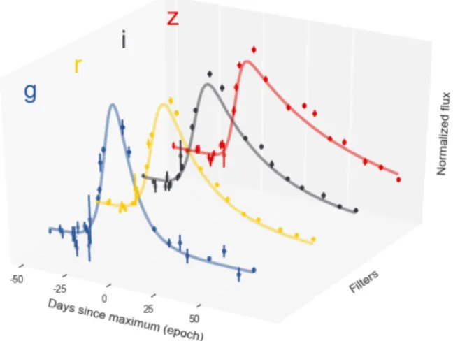
Figure 4. Example of light curve fitted with the parametric func-tion ofBazin et al.(2009) - equation1. The plot shows measure-ments for a typical well-sampled type Ia at redshift z ∼ 0.20, in each one of the 4 DES filters (dots and error bars) as well as its best fitted results (lines).
ture extraction method can significantly impact classifica-tion results (seeLochner et al. 2016, and references therein). In what follows, we use the parametrization proposed byBazin et al.(2009),
f (t)= A e −(t−t0)/τf
1+ e(t−t0)/τr + B,
(1) where A, B, t0, τf and τr are parameters to be
deter-mined. We fit each filter independently in flux space with a Levenberg-Marquardt least-square minimization (Madsen et al. 2004). Figure 4 shows an example of flux measure-ments, corresponding errors and best-fit results in all 4 filters for a typical, well-sampled, SN Ia from SNPCC data.
Although not optimal for such a diverse light curve sam-ple, the parametrization given by Eq.1was chosen for being a fast feature extraction method. Moreover, as any para-metric function, it returns the same number of parameters independently of the number of observed epochs, which is crucial for dealing with an inhomogeneous time-series which changes on a daily basis (the importance of this homoge-neous representation is further detailed in Section 5). We stress that a more flexible feature extraction procedure still holding the characteristics described above would only im-prove the results presented here.
3.2 Classifier
Once the data has been homogenized, we need a supervised learning model to harvest the information stored in the spec-troscopic sample. Analogous to the feature extraction case, the choice of classifier also impacts the final classification results for a given static data set (Lochner et al. 2016). In order to isolate the impact of AL in improving a given config-uration of feature extraction and machine learning pipeline, we chose to restrict our analysis to a single classifier. A com-plete study on how different classifiers respond to the update in training provided by AL is out of the scope of this work, but is a crucial question to be answered in subsequent stud-ies. All the results we present below were obtained with a random forest algorithm (Breiman 2001).
Random forest is a popular machine learning algorithm known to achieve accurate results with minimal parameter tuning. It is an ensemble technique made up of multiple de-cision trees (Breiman et al. 1984), constructed over different sub-samples of the original data. Final results are obtained by averaging over all trees (for further details, see appendices A and B ofRichards et al. 2012a). The method has been suc-cessfully used for SN photometric classification (Richards et al. 2012a;Lochner et al. 2016;Revsbech et al. 2017). In what follows, we used the scikit-learn11 implementation of the algorithm with 1000 trees. In this context, the prob-ability of being a SN Ia, pIa, is given by the percentage of trees in the ensemble voting for a SNIa classification12.
3.3 Metrics
The choice of a metric to quantify classification success goes beyond the use of classical accuracy (equation2) - especially when the populations are unbalanced (figure3). In order to optimize information extraction, this choice must take into account the scientific question at hand.
In the traditional SN case, the goal is to improve the quality of the final SNIa sample for further cosmological
11 http://scikit-learn.org/
12 In this work we are concerned only with Ia × non-Ia classifi-cation. The analysis of classification performance using other SN types will be the subject of a subsequent investigation.
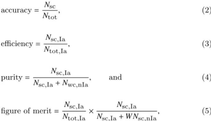
use. In this context, a false negative (a SNIa wrongly classi-fied as non-Ia) will be excluded from further analysis posing no damage on subsequent scientific results. On the other hand, a false positive (non-Ia wrongly classified as a Ia) will be mistaken by a standard candle, biasing the cosmologi-cal analysis. Thus, purity (equation 4) of the photometri-cally classified SNIa set is of paramount importance. At the same time, we wish to identify as many SNe Ia as possible (high efficiency - equation3), in order to guarantee optimal exploitation of our resources. Taking such constraints into consideration, Kessler et al. (2010) proposed the use of a figure of merit which penalizes classifiers for false positives (equation5). Throughout our analysis, classification results will be reported according to these 4 metrics:
accuracy= Nsc Ntot , (2) efficiency= Nsc,Ia Ntot,Ia , (3) purity= Nsc,Ia Nsc,Ia+ Nwc,nIa , and (4)
figure of merit= Nsc,Ia Ntot,Ia
× Nsc,Ia Nsc,Ia+ WNsc,nIa
, (5)
where Nsc is the toal number of successful classifications, Ntotthe total number of objects in the target sample, Nsc,Ia the number of successfully classified SNe Ia (true positives), Ntot,Ia the total number of SNe Ia in the target sample, Nwc,nIathe number of non-Ia SNe wrongly classified as SNe Ia (false positives) and W is a factor which penalizes the occurrence of false positives. FollowingKessler et al.(2010) we always use W= 3.
In the AL framework we propose, the metrics above are used to quantify the classification results in the target sample. They were calculated after the classifications were performed and had no part in the decision making algorithm (further details in Section4and AppendixA).
4 ACTIVE LEARNING
We now turn to the key missing ingredient in our pipeline. The tools we have described thus far allow us to process (section3.1), classify (section 3.2), and evaluate classifica-tion results (secclassifica-tion3.3) given a pair of labelled and unla-belled light-curve data sets. The question now is: starting from this initial configuration, how can we optimize the use of subsequent spectroscopic resources in order to maximize the potential of our classifier? Or in other words, how can we achieve high generalization performance by adding a mini-mum number of new spectroscopically observed objects to the training sample? We advocate the use of a dedicated rec-ommendation system tuned to choose the most informative objects in a given sample - those which will be spectroscop-ically targeted.
Active learning (AL) is an area of machine learning designed to optimize learning results while minimizing the number of required labelled instances. At each iteration, the
algorithm suggests which of the unlabelled objects would be most informative to the learning model if its label was avail-able (Settles 2012; Balcan et al. 2009; Cohn et al. 1996). Once identified, a query is made - in other words, the algo-rithm is allowed to interact with an external agent in order to ask for the label of that object13. The queried object -along with its label - is then added to the training sample and the model is re-trained. This process is repeated un-til convergence is achieved, or unun-til labelling resources are exhausted. The complete algorithm is illustrated in Fig.5.
Different flavours of AL propose different strategies to identify which objects should be queried. In what follows, we report results obtained using pool-based AL14via uncer-tainty sampling. In this framework, we start with two sets of data: labelled and unlabelled. At first, the machine learn-ing algorithm (classifier) is trained uslearn-ing all the available labelled data. Then, it is used to provide a class probabil-ity for all objects in the unlabelled set. The object whose classification is most uncertain is chosen to be queried. In a binary classification problem as the one investigated here, this corresponds to querying objects near the boundary be-tween the two classes - where the classifier is less reliable. A detailed explanation of the uncertainty sampling technique (as well as query by committee) is given in appendixA.
Finally, whenever one wishes to quantify the improve-ment in classification results due to AL, it is important to keep in mind that simply increasing the number of objects available for training changes the state of the model - in-dependently of how the extra data were chosen. Thus, AL results should always be compared to the passive learning strategy, where at each iteration objects to be queried are randomly drawn from the unlabelled sample. Moreover, in the specific case of SN classification, we also want to in-vestigate how the learning model would behave if the same number of objects were queried following the canonical spec-troscopic targeting strategy - where objects to be queried are randomly drawn from a sample which follows closely the initial SNPCC labelled distribution. Diagnostic results presented bellow show outcomes from all three strategies: canonical, passive learning, and AL via uncertainty sam-pling15.
4.1 Static full light curve analysis
We begin by applying the complete framework described in the previous subsections to static data. This is the tradi-tional approach, where we consider that all light curves were completely observed at the start of the analysis. Although this is not a realistic scenario (one cannot query, or spec-troscopically observe, a SN that has already faded away), it gives us an upper limit on estimated classification results. Section 5 considers more realistic constraints on available query data and light-curve evolution.
13 In the machine learning jargon, this agent is called an oracle. It can be a human, machine or piece of software capable of providing labels. In our context, making a query to the oracle corresponds to spectroscopically determining the class of a given object. 14 Our analysis used the libact Python package developed by Yang et al.(2017).
15 The code used in this paper can be found in the COINtoolbox -https://github.com/COINtoolbox/ActSNClass
Figure 5. Schematic illustration of the Active Learning (AL) work flow in the context of photometric light curves classification. Starting at the top left, the training set (spectroscopic sample -grey circles), is used to train a machine learning algorithm - re-sulting in a model which is then applied to the unlabelled data (photometric light-curves - yellow pentagons). This initial model returns a classification for each data point of the unlabelled set (now represented as red squares and blue triangles). The AL al-gorithm is then used to choose a data point of the unlabelled data with highest potential to improve the classification model (iden-tified by the grey arrow). The label of this point is then queried (a spectrum is taken). Once the true label of the queried point is known, it is added to the training set (converted into a grey circle), and the process is repeated.
For each light curve and filter, all available data points were used to find the best-fit parameters of equation1 fol-lowing the procedure described in section3. Best-fit values for different filters were concatenated to compose a line in the data matrix. In order to ensure the quality of fit, we considered only SNe with a minimum of 5 observed epochs in each filter; this reduced the size of our spectroscopic and photometric samples to 1094 and 20193 objects, respectively.
4.1.1 Sub-samples
The iterative framework presented above corresponds to the AL strategy for choosing the next object to be queried. In this description, we have 2 samples: labelled and unlabelled. In case we wish to quantify the performance of the ML al-gorithm after each iteration, the recently re-trained model must be used to predict the classes of objects in a third sam-ple –one that did not take part in the AL algorithm. Classifi-cation metrics are then calculated, after each iteration, from predictions on this independent sample. In this scenario we need 3 samples: training, query, and target. The query sam-ple corresponds to the set of all objects available for query
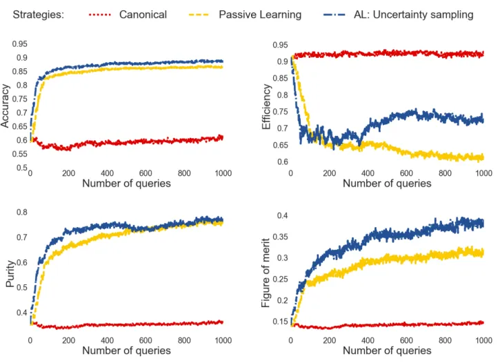
Figure 6. Evolution of classification results as a function of the number of queries for the static full light curve analysis.
upon which the model evolves16. On the other hand, the tar-get sample corresponds to the independent one over which diagnostics are computed. In the traditional analysis, query and target sample follow the same underlying distribution in feature space; this separation helps avoid overfitting. This is the case for the static full light curve analysis. In the results presented in this sub-section, SNPCC photo was randomly divided into query (80%) and target (20%) samples.
Finally, we quantified the evolution of the classification results when new objects are added to the training sample according to the canonical spectroscopic follow-up strategy, by constructing a pseudo-training sample. For each element of SNPCC spec, we searched for its nearest neighbour in SNPCC photo17. This allowed us to construct a data set which follows very closely the distribution in the parameter space covered by the original SNPCC spec. Thus, randomly drawing elements to be queried from this pseudo-training
16 Not to be confused with the set of queried objects, which com-prises the specific objects added to the training set (1 per itera-tion).
17 This calculation was performed in a 16 dimensions parameter space: type, redshift, simulated peak magnitude, and mean SNR in all 4 filters. For all the numerical features we used a standard euclidean distance.
sample is equivalent to feeding more data to the model ac-cording to the canonical spectroscopic follow-up strategy.
4.1.2 Results
In this section we present classification results for the static full light curve scenario according to 3 spectroscopic target-ing strategies: canonical, passive learntarget-ing and AL via uncer-tainty sampling (section4). In all three cases, at each itera-tion 1 object was queried and added to the training sample (the one with highest uncertainty). We allowed a total of 1000 queries, almost doubling the original training set.
Figure 6 shows how classification diagnostics evolve with the number of queries. The red inverse triangles de-scribe results following the canonical strategy (random sam-pling from the pseudo-training sample), yellow circles show results from passive learning (random sampling from the query sample), and blue triangles represent results for AL via uncertainty sampling. We notice that the canonical spec-troscopic targeting strategy does not add new information to the model –even if more labelled data is made available. Thus there is almost no change in diagnostic results after 1000 queries. On the other hand, the canonical strategy is very successful in identifying SN Ia (approximately 92% ef-ficiency); however, by prioritizing bright events, it fails to
Canonical Passive learning AL: Uncertainty sampling 18 21 24 27 18 21 24 27 18 21 24 27 900 700 500 250 100 50 40 30 20 10
i−band peak magnitude
Number of quer
ies
Training Target Queried objects
Figure 7. Simulated i-band peak magnitude distribution as a function of the number of queries for the static full light curve scenario. The yellow (blue) region shows distribution for the training (target) samples, while the red curves denote the composition of sample queried by AL. Lines go through 10 to 900 queries (from top to bottom). Different columns correspond to different learning strategies: canonical, passive and active learning via uncertainty sampling (from left to right).
provide the model with enough information about other SN types. Consequently, its performance in other diagnostics is poor (∼ 60% accuracy, 36% purity and a figure of merit of 0.15). At the same time, passive learning and AL via un-certainty sampling show very similar efficiency results up to 400 queries. Accuracy levels stabilize quickly (84%/87% af-ter only 200 queries), followed closely by purity results (73% after 600 queries). The biggest difference appears on effi-ciency levels. We can recognize an initial drop in effieffi-ciency up to 400 queries. This is expected, since both strategies pri-oritize the inclusion of non-Ia objects in the training sample: passive learning simply led by the higher percentages of non-Ia SNe in the target sample (figure3), and AL by aiming at a more diverse information pool. This implies that high accuracy and purity levels are accompanied by a decrease in efficiency (from 92% to 68% at 200 queries). After a mini-mally diverse sample is gathered, passive learning continues to lose efficiency, stabilizing at 63% after 700 queries, while
AL is able to harvest further information to stabilize at 72% after 800 queries. Thus, after 1000 new objects were added to the training sample, passive learning achieves a figure of merit of 0.32 (2.1 times higher than canonical), while AL via uncertainty sampling achieves a figure of merit of 0.39 (2.6 times higher than canonical).
Figure7illustrates how the distribution of peak i-band magnitude in the set of queried elements evolves with the number of queries. For the sake of comparison, we also show the static distributions for the training (yellow) and target (blue) samples. As expected, the canonical strategy consis-tently follows the spectroscopic sample distribution. Mean-while, passive learning completely ignores the existence of the initial training –consequently, its initial queries overlap with regions already covered by the training sample, allo-cating a significant fraction of spectroscopic resources to ob-tain information already available in the training. The AL strategy, even in very early stages, takes into account the
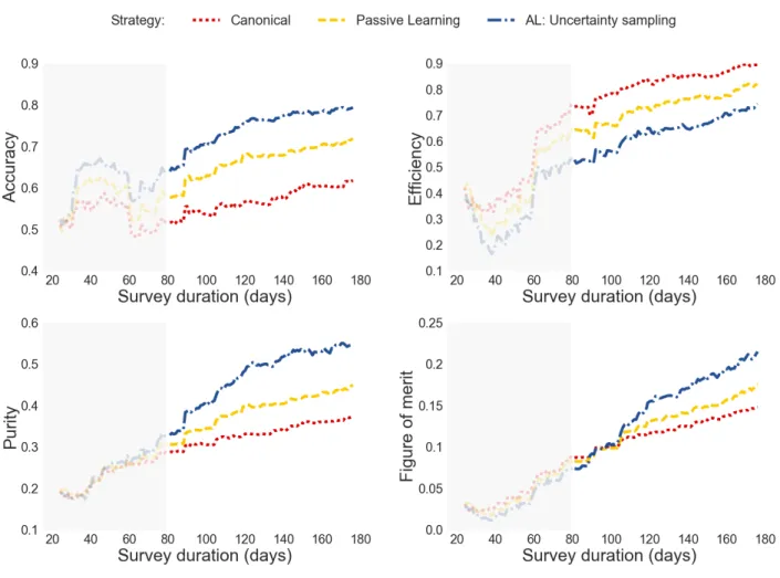
Figure 8. Evolution of the classification results as a function of the survey duration for the time-domain AL considering the SNPCC training set as completely given in the beginning of the survey.
existence of the training sample, focusing its queries in the region not covered by training data (higher magnitudes). At 900 queries, the set of queried objects chosen by passive learning (red line, middle column) follows closely the distri-bution found in the target sample (blue), - but this does not translate into a better classification because the bias present in the original training was not yet overcome. On the other hand, the discrepancy in distributions between the target sample (blue region) and the set of objects queried by AL (red line, right-most column) at 900 queries is a consequence of the existence of the initial training18. The fact that AL takes this into account is reflected in the classification results (figure6).
These results provide evidence that AL algorithms are able to improve SN photometric classification results over canonical spectroscopic follow-up strategies, or even passive learning in a highly idealized environment19. However, in order to have a more realistic description of a SN survey, we
18 The reader should keep in mind that after 1000 queries the model is trained in a sample containing the complete SNPCC spectroscopic sample added to the set of queried objects. 19 A result already pointed out byGupta et al.(2016).
need to take into account the transient nature of the SNe and the evolving aspect of an observational survey.
Although we chose to illustrate non-representativeness between samples in terms of peak brightness in different bands (e.g. figures1,7and 12), these features are absence in the input data matrix. Our goal is to emphasize that the underlying astrophysical properties are tracked differently by the AL and passive learning strategies - even if these are not explicitly used.
5 REAL-TIME ANALYSIS
In this section, we present an approach to deal with the time evolving aspect of spectroscopic follow-ups in SN surveys. This is done through the daily update of:
(i) identification of objects allocated to query and target samples,
(ii) feature extraction and (iii) model training.
We begin considering the full SNPCC spectroscopic sample completely observed at the beginning of the survey - this allows us to have an initial learning model. Then, at
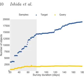
Figure 9. Number of objects in the query (yellow circles) and target (blue triangles) samples as a function of the days of survey duration. The grey region highlights the initial build-up phase of the survey, where there is a steep increase in the number of objects in the target sample.
each observation day d, a given SN is included in the analy-sis if, until that moment, it has at least 5 observed epochs in each filter. If this first criterion is fulfilled, the object is des-ignated as part of the query sample if its r-band magnitude is lower than or equal to 24 (mr ≤ 24 at d) - otherwise, it is assigned to the target sample20. Figure9shows how the number of objects in the query (yellow circles) and target (blue triangles) samples evolves as a function of the num-ber of observing days. Although the survey starts observing at day 1, we need to wait until day 20 in order to have at least 1 object with a minimum of 5 observed epochs in each filter. From then on, the query sample begins with 666 ob-jects (at day 20) and shows a steady increase until it almost stabilizes ∼ 2100 SNe (around day 60). On the other hand, the target sample shows a steep increase until d ∼ 80 (here-after, build-up phase) and continuous to grow from there until the end of the survey - although at a lower rate. This behaviour is expected since, in this description, the query sample corresponds to the fraction of photometric objects satisfying the magnitude threshold (mr ≤ 24) at a specific time. Notice that as the survey evolves, an object whose de-tection happened in a very early phase will be assigned to the target sample during its rising period, but if its bright-ness increases enough to allow spectroscopic targeting it will move to the query sample - where it will remain for a few epochs. After its maximum passes, the SN will eventually return to the target sample as soon as it fades below the magnitude threshold - remaining there until the end of the survey. Thus, it is important to keep in mind that, despite its size being practically constant after the build-up phase, individual objects composing the query sample might not be the same for consecutive days.
The feature extraction process is also performed on
20 We consider an object with r-band magnitude of 24 to have the minimum brightness necessary to allow spectroscopic observation with a 8-meter class telescope.
a daily basis, considering only the epochs measured un-til that day. This clarifies why we consider an analytical parametrization a simple, and efficient enough, feature ex-traction procedure. It reasonably fast and encompasses prior domain knowledge on light curve behaviour while returning the same number of parameters independently of the num-ber of observed epochs. Moreover, it avoids the necessity of determining the time of maximum brightness or performing any type of epoch alignment (see e.g.Richards et al. 2012a; Ishida & de Souza 2013; Revsbech et al. 2017). Thus, we are able to update the feature extraction step as soon as a new epoch is observed and still construct a homogeneous and complete low-dimensionality data matrix. The only con-straint is the number of observed epochs, which must be at least equal to the number of parameters in all filters.
Finally, at the end of each night, the model is trained using the features and labels available until that point. The AL algorithm is allowed to query only the objects belonging to the query sample. Once a query is made, the targeted object and corresponding label are added to the training sample, the model is re-trained and the result applied to the target sample (figure5). Given the time span of the SNPCC data, we are able to repeat this analysis for a total of 180 days.
Figure 8 shows the evolution of classification results considering the complete SNPCC spectroscopic sample as a starting point. Here we can clearly see the effect of the evolving sample sizes: accuracy and efficiency results oscil-late, while purity and figure of merit remain indifferent to the learning strategy, during the build-up phase (grey re-gion). Once this phase is over, results start to differ and the AL with uncertainty sampling clearly surpasses the other two, achieving 80% accuracy, 55% purity and a figure of merit of 0.23, while the passive learning only goes up to 72% accuracy, 45% purity and figure of merit of 0.18. The canonical strategy continues to output better efficiency, but its loss in purity does not allow it to overcome even passive learning in figure of merit levels.
5.1 No initial training
This leaves one open question: what should we do at the beginning of a given survey, when a training set with the same instrument characteristics (e.g. photometric system) is not yet available? Or even more drastically: if the algorithm is capable of building its own training sample, do we even need an initial training at all? The answer is no.
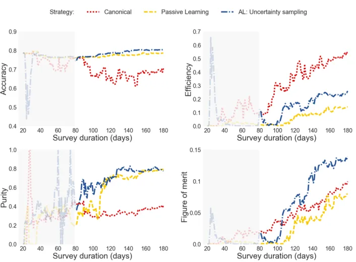
Figure 10 shows how the classification results behave when the initial model is trained in 1 randomly selected ob-ject from the query sample, meaning we start with a random classifier. In this context, diagnostics are meaningless until around 100 days (a little after the build-up phase) when all samples involved are under construction. After this period, AL with uncertainty sampling starts to dominate purity and, consequently, figure of merit results. After 150 observation days (or after 130 objects were added to the training), the active and passive learning strategies achieve purity levels comparable to the one obtained in the unrealistic full light curve scenario (∼ 80%). Thus, at the end of the survey, AL efficiency results (27%) are 80% higher than the one ob-tained by passive learning (15%), which translates into an almost doubled figure of merit (0.14 from AL and 0.08 from
Figure 10. Evolution of classification results as a function of survey duration in the real time analysis, with a random initial training of 1 object.
the canonical strategy). Compare these results with the ini-tial state of the full light curve analysis: figure6(accuracy 60%, efficiency 92%, purity of 35% and 0.15 figure of merit) was obtained using complete light curves for all objects, all SNe in the original SNPCC spectroscopic sample surviving the minimum number of epochs cuts (1094 objects) and the same random forest classifier. Final results of the real-time AL analysis (figure 10) surpasses the full light curve initial state accuracy results in 33%, more than doubles purity and achieves comparable figure of merit results. All of these while respecting the time evolution of observed epochs of only 161 SNe in the training set, or 15% the number of objects in the original SNPCC spectroscopic sample.
Accuracy levels of real time AL with (figure8) and with-out (figure10) the full initial training sample are compara-ble, while efficiency and figure of merit are higher for the former case. However, purity levels are 45% higher without using the initial training. This is a natural consequence of the higher number of SNe Ia in the SNPCC spectroscopic sample (figure 9), which requires the algorithm to unlearn the preference for Ia classifications before it can achieve its full potential in purity results. Figure10also shows that re-garding purity, passive learning is able to achieve the same results as those obtained with uncertainty sampling while
efficiency is severely compromised –exactly the opposite be-haviour shown by the canonical strategy. This is a conse-quence of the populations targeted by each of these strate-gies. By prioritizing brighter objects, the canonical strategy introduces a bias in the learning model towards SNIa clas-sifications. On the other hand, by randomly sampling from the target, passive learning adds a larger number of non-Ia examples to the training, introducing an opposite bias, at least in the early stages of the survey.
In summary, given the intrinsic bias present in all canon-ically obtained samples, we advocate that the best strategy for a new survey is to construct its own training during the firsts running seasons. Letting its own photometric sample guide the decisions of spectroscopic targeting. This is spe-cially important if one has the final goal of supernova cos-mology in mind, where the main objective is to maximize purity (minimize false positives) as well as many other sci-entific SN objectives.
6 BATCH-MODE ACTIVE LEARNING
In this section, we take another step towards a more realistic description of a spectroscopic follow-up scenario. Instead of choosing one SN at a time, spectroscopic follow-up resources
Figure 11. Evolution of classification results as a function of survey duration for the batch-mode real time analysis with N= 5 and a random initial training of 5 objects.
for large scale surveys will probably allow a number of SNe to be spectroscopically observed per night. Thus, we need a strategy which allows us to extend the AL algorithm, opti-mizing our choice from one to a set (or a batch) of objects at each iteration. We focus on two methods derived from the notion of uncertainty sampling: N-least certain and Semi-supervised uncertainty sampling.
The N-least certain batch query strategy uses the same machinery described in the sequential uncertainty sampling method but, instead of choosing a single unlabelled exam-ple, it selects the N objects with highest uncertainties, and queries all of them. This tactic carries a disadvantage, since a set of objects whose predictions exhibit similar uncertainties will probably also be similar among themselves (i.e., will be close to each other in the feature space). Thus, querying for a set of labels is not likely to lead to a model much different than the one obtained by adding only the most uncertain object to the training set. In dealing with a batch mode sce-nario, we should also require that the elements of the batch be as diverse as possible (maximizing their distance in the feature space).
Semi-supervised uncertainty sampling (e.g. Hoi et al. 2008), in contrast, avoids the need to call the oracle at each individual iteration by using the uncertainty associated to
each predicted label as a proxy for class assignment. The algorithm must be trained in the available initial sample in order to create the first batch. The object with the great-est classification uncertainty is then identified. Suppose this object has a probability p of being SN Ia. A pseudo-label is then drawn from a Bernoulli distribution, where success is interpreted as “Ia” label (with probability p) and failure as “non-Ia” (with probability 1−p). The object features and cor-responding pseudo-label are temporarily added to the train-ing sample and the model is re-trained. This is repeated until we reach the size of the batch (see algorithm1). The benefit of using the model to produce pseudo-labels comes with the inevitable uncertainty attached to model predictions: they come unwarranted. However, the problem attached to the N-least certain strategy is here, to a certain degree, overcome. Similar unlabelled instances are less likely to be included in the same batch.
The optimum number of elements in each batch, N, is highly dependent on the particular combination of data set and classifier at hand. At each iteration, we are actually stretching the capabilities of the learning model in a feed-back loop that cannot be expected to perform well for large batches. For the SNPCC data, our tests show that
semi-supervised learning outperforms the N-least certain strategy for N ∈ [2, 8] with maximum results obtained with N= 5.
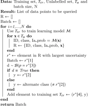
Data: Training set, Ttr, Unlabelled set, Tu and batch size, N
Result: List of data points to be queried R ← []
Batch ← [] for i=1,...,N do
Use Ttr to train learning model M for x ∈ Tu do
ID, class, Ia prob = M(x) R ← {ID, class, Ia prob, x} end
r∗← element in R with largest uncertainty Batch ← r∗[1] d ∼ B(p= r∗[3]) if d ≡ True then y ← r∗[2] else y ← alternate class (, r∗[2]) end
Add element to training set Ttr← (r∗[4], y) end
return Batch
Algorithm 1: Semi-supervised uncertainty sampling al-gorithm to identify which elements must be included in the batch.
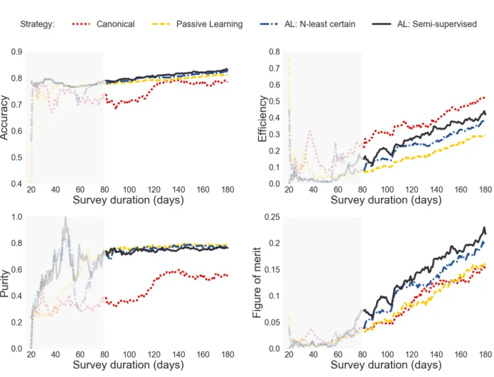
Figure11shows classification results for canonical and passive learning (both at each iteration drawing 5 random elements from the pseudo-training and target sample respec-tively), AL via N-least certain and semi-supervised uncer-tainty sampling, when the initial training consists of 5 ran-domly drawn objects from the query sample and N = 5. We see that in this scenario semi-supervised AL is able to achieve the same figure of merit (∼ 0.22) as sequential un-certainty sampling when the entire initial training sample is available (figure 8). However, it does so using only 63% of the number of objects for training (or 800 SNe in the training after 180 days, against 1263 SNe in the full training case). Moreover, although efficiency results show a steady increase until the end of the survey, purity achieves satu-ration levels (∼ 0.8 - the same as the final results obtained with the static full light curve scenario, figure6) after only 100 days (corresponding to a training set with 405 objects). A numerical description of the final classification results and corresponding training size is shown in table1.
From figure11we see that samples containing the same number of objects lead to different classification results. Moreover, considering that the query sample only contains objects with mr ≤ 24, we should not expect the set of objects queried by AL to be representative of the target sample, de-spite the improvement in classification results driven by AL. This is clearly shown in figure12, where we compare distri-bution of maximum observed brightness in each filter for the SNPCC spectroscopic (red) and photometric (blue) samples with the set of objects queried by AL (dark grey). The latter provides a slight advantage in coverage when compared to the original spectroscopic sample, but it is still significantly different from the photometric distribution. A similar be-haviour is found when we compare the populations of
differ-ent SN types (figure13) and redshift distribution (figure14). These results confirm that, although a slight adjustment is necessary in order to optimize the allocation of spectroscopic time, a significant improvement in classification results may be achieved without a fully representative sample.
7 TELESCOPE ALLOCATION TIME
As a final remark, we must address the question of how much spectroscopic telescope time is required to obtain the labels queried by the AL algorithm – in comparison to the time necessary to get all labels from SNPCC spectroscopic sample (canonical strategy).
In the realistic case of a survey adoption of the frame-work proposed here, a term taking into account the telescope time needed for spectroscopy observations must be added to the cost function of the AL algorithm. This was not explic-itly taken into account in this paper, but we considered a constraint on magnitudes for the set of SNe available for spectroscopic follow-up (rmag ≤ 24). We were able to esti-mate the integration time required for each object to achieve a given SNR by considering its magnitude and typical values for statistical noise of the sources21. In the SNPCC spectro-scopic sample, we considered the spectra taken at maximum brightness. For the set of AL queried objects, we used the magnitude at the epoch in which the object was queried. Considering a SNR of 10 (more than enough to enable clas-sification) the ratio between the total spectroscopic time needed to get the labels for the SNPCC spectroscopic sam-ple and the set of objects queried by semi-supervised AL is 0.9992. This indicates that the set of objects queried by AL would require less than 2.9s more time than the SNPCC spectroscopic sample to be observed at each hour. Also, if a more realistic estimation had been performed considering instrumental overheads, the set of objects queried by AL would have significant advantage, as it contains 26% less ob-jects than the SNPCC spectroscopic sample. This gives us the first indication that AL-like approaches are feasible al-ternatives to minimize instrumental usage and, at the same time, optimize scientific outcome of photometrically classi-fied samples.
For the specific case studied here, the high purity values achieved in early stages of the batch-mode AL, accompanied by the steady increase in efficiency (figure11) renders our final SN Ia sample optimally suited for photometric clas-sification in cosmological analysis –albeit being smaller in number of objects and requiring almost the same amount of spectroscopic resources to be secured.
8 CONCLUSIONS
Wide-field sky rolling surveys will detect an unprecedented number of astronomical transients every night. However, the usefulness of these photometric data for cosmological anal-ysis is conditioned on our ability to perform automatic and reliable light-curve classification using a very limited num-ber of spectroscopic observations for validation. Traditional
21 Namely, counts in the sky, ≈ 13.8 e−/s/pix and read-out noise, ≈ 8 e−(e.g.Bolte 2015).
static, full LC time domain time domain
time domain initial training initial training initial training
UNC UNC BATCH 5 BATCH 5
training 2093 1255 1093 810 size accuracy 0.89 0.80 0.85 0.83 efficiency 0.73 0.78 0.69 0.44 purity 0.78 0.55 0.69 0.76 figure of merit 0.39 0.23 0.31 0.22
Table 1. Classification results for the AL by uncertainty sampling (UNC) and semi-supervised batch mode (BATCH 5) strategies.
Figure 12. Distributions of maximum observed brightness, in all DES filters, for the set of objects queried by AL via batch-mode semi-supervised uncertainty sampling with N = 5 (dark grey). This is compared to distributions from SNPCC spectroscopic (red - top) and SNPCC photometric (blue - bottom) samples.
attempts to address this issue via supervised learning meth-ods focus on a learning model that postulates a static, fully observed pair of spectroscopic (training) and photometric (target) samples. Such studies are paramount to assess the requirements and performance of different classifiers. Nev-ertheless, they fail to address fundamental aspects of as-tronomical data acquisition, which renders the problem ill-suited for text-book machine learning algorithms. The most crucial of these issues is the non-representativeness between spectroscopic and photometric samples.
This mismatch has its origins in a follow-up strategy designed to maximize the number of spectroscopically con-firmed SNe Ia for cosmology, resulting in a highly biased spectroscopic set — and a sub-optimal training sample. Given such data configuration, not even the most suitable classifier can be expected to achieve its full potential. In this work, we advocate that any attempt to improve SN pho-tometric classification must include a detailed strategy for constructing a more representative training set, without ig-noring the constraints intrinsic to the observational process. Our proposed framework updates on a daily basis cru-cial steps of the SN photometric classification pipeline and
Sample SN type SNPCC train AL query SNPCC photo Ia Ibc II SNPCC photo AL: semi SNPCC spec Ia Ibc II Sample SNe type
Figure 13. Populations of different supernova types in the orig-inal SNPCC spectroscopic and photometric samples, and in time domain batch mode (N = 5) semi-supervised AL query sample after 180 days of observations. The composition of the SNPCC samples are the same as shown in figure3. The AL query sample holds 390 (48%) Ia, 122 (15%) Ibc and 298 (37%) II.
uses active learning to optimize the scientific outcome from machine learning algorithms. On each day, we consider only the set of available observed epochs, and perform feature extraction via a parametric light-curve representation. The identification of SNe available for spectroscopic targeting (objects with mr ≤ 24 on that day) as a separate group from the full photometric sample is also updated daily. Fi-nally, by using Active Learning (AL), we allow the algo-rithm itself to target those objects available for spectro-scopic targeting that would maximally improve the learn-ing model if added to the trainlearn-ing set. Uslearn-ing the proposed semi-supervised batch-mode AL, we designate an optimal set of new objects to be spectroscopically observed on each night. Once the batch is identified, the model is re-trained and new spectroscopic targets are selected for the subse-quent night. This method avoids the necessity of an initial training sample: it starts with a random classifier, allow-ing the algorithm to construct an optimal trainallow-ing sample
Figure 14. Redshift distribution of the original SNPCC spectro-scopic (red - dotted) and photometric (blue - dashed) samples, superimposed to the redshift distribution of the AL query set for the time domain semi-supervised batch mode AL strategy with-out the use of an initial training (dark blue - full). In each obser-vation night, the algorithm queried for 5 SNe. The distribution shows redshift for the query sample after 180 observation nights. .
from scratch, specifically adapted to the survey at hand. The framework was successfully applied to the simulated data re-leased after the Supernova Photometric Classification Chal-lenge (SNPCCKessler et al. 2010).
Our results show that the proposed framework is able to achieve high purity levels, ∼ 80%, after only 100 observation days — which corresponds to a training set of only 400 ob-jects. After 180 observation days, or 800 queries, we are able to reach a figure of merit of 0.22 (figure11) — highly above the values we would have obtained by using the canonical strategy for the idealized full training and full light curve analysis (which achieves 35% purity and figure of merit of 0.14, red curve in figure6).
After showing the classification improvements achieved with the AL algorithm, we examined the characteristics of the set of objects queried by AL. As expected, the mr ≤ 24 requirement does not allow this set to deviate strongly from the characteristics of the SNPCC spectroscopic sample (see figures 12, 14 and 13). However, these small differences translate into significant improvements in purity, and conse-quently, figure of merit results. This comes with no penalty whatsoever in the necessary observational time for spectro-scopic follow-up. The ratio of integration times required to observe the complete set of queried objects and the SNPCC spectroscopic sample is close to unity. This is still additional evidence that Active Learning is a viable strategy to opti-mize the distribution of spectroscopic resources.
In all our results, we observe that the canonical target-ing strategy, which prioritizes the spectroscopic follow-up of bright events which resemble SNe Ia, has higher efficiency results (which means that this strategy is more successful in identifying a high number of SNe Ia in the target sample). However, as the diversity present in the training sample is very low, purity levels are always compromised. The canon-ical strategy is successful in targeting SNe Ia, but it is not
optimal when the goal is to construct a training sample for machine learning classifiers.
In the present analysis, we restricted ourselves to the SNe photometric classification case of SNe Ia versus non-Ia. However, we stress that our methodology is easily adaptable to more general classifications that include other transients (e.g. Narayan et al. 2018). This exercise will be especially informative when applied to the data from the upcoming Photometric LSST Astronomical Time-series Classification Challenge22(PLAsTiCC).
Finally, it is reasonable to expect that different combi-nations of classifiers and feature extraction methods will re-act differently to the iterative AL process. The same is valid for the AL algorithm itself. Moreover, there are other prac-tical issues that we did not take into account, like the time delay necessary to treat the spectra and provide a classifica-tion or the fact that sometimes one spectra is not enough to get a classification. In summary, we recognize that each item in our pipeline can be refined, potentially leading to even more drastic improvements in classification results. The re-sults we show here are the first evidence that an iterative learning process adapted to the specificities of astronomi-cal observations can lead to significant optimization in the allocation of observational resources.
Adapting to the era of big data in astronomy will entail adapting machine learning techniques to the unique reality of astronomical observations. This requires tackling funda-mental issues which will always be present in astronomical data (e.g. the discrepancy between training and test sam-ples and the time evolution of a transient survey). Astron-omy has once again the opportunity to provide ground for developments in other research areas by providing unique data situations not commonly present in other scenarios, as long as a consistent interdisciplinary environment is avail-able. We are convinced that the most exciting part of this endeavour is still to come.
ACKNOWLEDGEMENTS
This work was created during the 4th COIN Residence Pro-gram23(CRP#4), held in Clermont-Ferrand, France on Au-gust 2017, with support from Universit´e Clermont-Auvergne and La R´egion Auvergne-Rhˆone-Alpes. This project is finan-cially supported by CNRS as part of its MOMENTUM pro-gramme over the 2018-2020 period. EEOI thanks Michele Sasdelli for comments on the draft and Isobel Hook for useful discussions. AKM acknowledges the support from the Portuguese Funda¸c˜ao para a Ciˆencia e a Tecnologia (FCT) through grants SFRH/BPD/74697/2010, from the Portuguese Strategic Programme UID/FIS/00099/2013 for CENTRA, the ESA contract AO/1-7836/14/NL/HB and Caltech Division of Physics, Mathematics and Astronomy for hosting a research leave during 2017-2018, when this paper was prepared. RSS thanks the support from NASA under the Astrophysics Theory Program Grant 14-ATP14-0007. RB acknowledges support from the National Sci-ence Foundation (NSF) award 1616974 and the NKFI NN
22 https://plasticcblog.wordpress.com/ 23 https://iaacoin.wixsite.com/crp2017
114560 grant of Hungary. BQ acknowledges financial support from CNPq-Brazil under the process number 205459/2014-5. AZV acknowledges financial support from CNPq. AM thanks partial support from NSF through grants AST-0909182, AST-1313422, AST-1413600, and AST-1518308. This work has made use of the computing facilities of the Laboratory of Astroinformatics (IAG/USP, NAT/Unicsul), whose purchase was made possible by the Brazilian agency FAPESP (grant 2009/54006-4) and the INCT-A. This work was partly supported by the Center for Advanced Comput-ing and Data Systems (CACDS), and by the Texas Insti-tute for Measurement, Evaluation, and Statistics (TIMES) at the University of Houston. This project has been sup-ported by a Marie Sklodowska-Curie Innovative Train-ing Network Fellowship of the European Commission’s Horizon 2020 Programme under contract number 675440 AMVA4NewPhysics.
The Cosmostatistics Initiative24(COIN) is a non-profit organization whose aim is to nourish the synergy between as-trophysics, cosmology, statistics, and machine learning com-munities. This work benefited from the following collabora-tive platforms: Overleaf25, Github26, and Slack27.
REFERENCES
Balcan M. F., Beygelzimer A., Langford J., 2009, Journal of Com-puter and System Sciences, 75, 78
Bazin G., et al., 2009,A&A, 499, 653 Betoule M., et al., 2014,A&A,568, A22
Bolte M., 2015, Modern Observational Techniques,http://www. ucolick.org/~bolte/AY257/s_n.pdf
Breiman L., 2001, Machine Learning, 45, 5
Breiman L., Friedman J. H., Olshen R. A., Stone C. J., 1984, Classification and Regression Trees. Wadsworth and Brooks, Monterey, CA
Campbell H., et al., 2013,ApJ,763, 88 Charnock T., Moss A., 2017,ApJ,837, L28
Childress M. J., et al., 2017, preprint, (arXiv:1708.04526) Cohn D. A., Ghahramani Z., Jordan M. I., 1996, Journal of
Ar-tificial Intelligence Research, 4, 129 Conley A., et al., 2011,ApJS,192, 1
Cover T. M., Thomas J. A., 2006, Elements of Information Theory (Wiley Series in Telecommunications and Signal Processing). Wiley-Interscience
Dai M., Kuhlmann S., Wang Y., Kovacs E., 2017, preprint, (arXiv:1701.05689)
DeBarr D., Wechsler H., 2009, in Sixth Conference on Email and Anti-Spam. Mountain View, California. pp 1–6
Foley R. J., Mandel K., 2013,ApJ,778, 167 Gamow G., 1948,Nature,162, 680
Goobar A., Leibundgut B., 2011,Annual Review of Nuclear and Particle Science,61, 251
Gupta K. D., Pampana R., Vilalta R., Ishida E. E. O., de Souza R. S., 2016, in 2016 IEEE Symposium Series on Computa-tional Intelligence (SSCI).
Hillebrandt W., Niemeyer J. C., 2000,Annual Review of Astron-omy and Astrophysics, 38, 191
Hlozek R., et al., 2012,ApJ,752, 79
24 https://github.com/COINtoolbox 25 https://www.overleaf.com 26 https://github.com 27 https://slack.com/
Hoi S. C. H., Jin R., Zhu J., Lyu M. R., 2008, in 2008 IEEE Con-ference on Computer Vision and Pattern Recognition. pp 1–7, doi:10.1109/CVPR.2008.4587350
Hoyle B., Paech K., Rau M. M., Seitz S., Weller J., 2016,MNRAS, 458, 4498
Ishida E. E. O., de Souza R. S., 2013,MNRAS,430, 509 Johnson B. D., Crotts A. P. S., 2006,AJ,132, 756 Jones D. O., et al., 2017,ApJ,843, 6
Karpenka N. V., Feroz F., Hobson M. P., 2013, MNRAS,429, 1278
Kessler R., et al., 2010,Publications of the Astronomical Society of Pacific,122, 1415
Kranjc J., Smailovi´c J., Podpeˇcan V., Grˇcar M., ˇZnidarˇsiˇc M., Lavraˇc N., 2015, Information Processing & Management, 51, 187
Kuznetsova N. V., Connolly B. M., 2007,ApJ,659, 530 Liu Y., 2004, Journal of chemical information and computer
sci-ences, 44, 1936
Lochner M., McEwen J. D., Peiris H. V., Lahav O., Winter M. K., 2016,ApJS,225, 31
Madsen K., Nielsen H. B., Tingleff O., 2004, Methods for Non-Linear Least Squares Problems (2nd ed.)
Masters D., et al., 2015,ApJ,813, 53
M¨oller A., et al., 2016,J. Cosmology Astropart. Phys.,12, 008 Narayan G., et al., 2018, preprint, (arXiv:1801.07323) Naul B., Bloom J. S., P´erez F., van der Walt S., 2018, Nature
Astronomy,2, 151
Newling J., et al., 2011,MNRAS,414, 1987 Perlmutter S., et al., 1999,ApJ,517, 565 Perrett K., et al., 2010,AJ,140, 518 Phillips M. M., 1993, ApJ, 413, L105
Planck Collaboration et al., 2016,A&A,594, A1
Poznanski D., Gal-Yam A., Maoz D., Filippenko A. V., Leonard D. C., Matheson T., 2002,PASP,114, 833
Poznanski D., Maoz D., Gal-Yam A., 2007,AJ,134, 1285 Revsbech E. A., Trotta R., van Dyk D. A., 2017, preprint,
(arXiv:1706.03811)
Richards J. W., Homrighausen D., Freeman P. E., Schafer C. M., Poznanski D., 2012a,MNRAS,419, 1121
Richards J. W., et al., 2012b,ApJ,744, 192 Riess A. G., et al., 1998,AJ,116, 1009
Rodney S. A., Tonry J. L., 2009,ApJ,707, 1064 Sako M., et al., 2008,AJ,135, 348
Settles B., 2012, Active Learning. Morgan & Claypool
Solorio T., Fuentes O., Terlevich R., Terlevich E., 2005,MNRAS, 363, 543
Spergel D. N., et al., 2007,ApJS,170, 377 Sullivan M., et al., 2006,AJ, 131, 960
Thompson C. A., Califf M. E., Mooney R. J., 1999, in ICML. pp 406–414
Tripp R., 1998, A&A, 331, 815
Varughese M. M., von Sachs R., Stephanou M., Bassett B. A., 2015,MNRAS,453, 2848
Vilalta R., Ishida E. E. O., Beck R., Sutrisno R., de Souza R. S., Mahabal A., 2017, in 2017 IEEE Symposium Series on Com-putational Intelligence (SSCI).
Wang Y., Gjergo E., Kuhlmann S., 2015,MNRAS,451, 1955 Xia X., Protopapas P., Doshi-Velez F., 2016, Cost-Sensitive Batch
Mode Active Learning: Designing Astronomical Observation by Optimizing Telescope Time and Telescope Choice. pp 477– 485,doi:10.1137/1.9781611974348.54
Yang Y.-Y., Lee S.-C., Chung Y.-A., Wu T.-E., Chen S.-A., Lin H.-T., 2017, preprint, (arXiv:1710.00379)