Alkenone-based evidence of Holocene slopewater cooling in the northwest Atlantic

Alkenone-based Evidence of Holocene Slopewater

Cooling in the Northwest Atlantic

by

Jessie M. Kneeland

B.S. Geology

California Institute of Technology,

2004

MASSACHUS• S IN

OF TECHNOLOGY

DEC 0 5 2006

LIBRARIES

Submitted to the Department of Earth, Atmospheric, and Planetary

Sciences

in partial fulfillment of the requirements for the degree of

Master of Science in Climate Physics and Chemistry

at the

MASSACHUSETTS INSTITUTE OF TECHNOLOGY

September 2006

©

Massachusetts Institute of Technology 2006. All rights reserved.

ARCHIVES

A uthor ...

-

" ...

...

DepartmBtit of Earth, Atmospheric, and Planetary Sciences

August 11, 2006

Certified by..,.

/ '

Accepted by ...

... y... ...

Julian P. Sachs

Associate Professor

Thesis Supervisor

.... ;.. .. .. ...

Maria T. Zuber

E.A. Griswold Professor of Geophysics

Head, Department of Earth, Atmospheric and Planetary Sciences

Alkenone-based Evidence of Holocene Slopewater Cooling in

the Northwest Atlantic

by

Jessie M. Kneeland

B.S. Geology

California Institute of Technology, 2004

Submitted to the Department of Earth, Atmospheric, and Planetary Sciences on August 11, 2006, in partial fulfillment of the

requirements for the degree of

Master of Science in Climate Physics and Chemistry

Abstract

Alkenone-based estimates of sea surface temperature (SST) in the northwest Atlantic during the last 10,000 years are presented and used to assess scenarios for Holocene climate variability. Alkenone concentration and unsaturation records are presented from cores KNR140-39GGC, KNR140-51GGC, 2028, 2031, and MD95-2025 from the Blake Ridge (32°N), Carolina Slope (330_{N), Fogo Seamount (42}0_N),

Narwhal (440_{N), and Orphan Basin (50'N) respectively. The southernmost core,} from the Blake Ridge, indicates very little temperature variation over the Holocene. Somewhat inshore and to the north of that location, the Carolina Slope record shows a slight cooling trend of about 1.50C over the past 5,000 years, which is interrupted by a brief but sudden drop of about 10_{C between 3,000 and 2,000 years before present.} Lack of age control for the core from Fogo Seamount prevents any conclusions about the time frame of alkenone variation at that location. At the Narwhal site, which is not far from the Laurentian fan, a strong and consistent cooling of 90_{C is the most} recent pattern of variation. Alkenone concentrations from the Orphan Basin were not sufficient for reliable measurement of a Holocene temperature trend. The general pattern of strong cooling in the northern slope water region and very modest cooling south of Cape Hatteras, where the Gulf Stream separates from the coastline and heads out to sea, may suggest a shift in mean Gulf Stream path as a possible culprit for the temperature record seen at the Narwhal site. However, changes of incoming solar radiation or seasonality of alkenone production over the Holocene provide alternative mechanisms for alkenone temperature variation.

Thesis Supervisor: Julian P. Sachs Title: Associate Professor

Acknowledgments

I wish to thank my advisors, Julian Sachs and Carl Wunsch, for the guidance and knowledge they provided while I prepared for and completed this thesis. Carl encour-aged me to take a critical look at the usual assumptions made in paleoceanography, and to be scientifically rigorous in my thinking. Julian provided an abundance of enthusiasm and plenty of ideas and access to samples to keep me busy.

I am very grateful to Carl for securing funding for my studies and work on this project; NASA is thanked for this support. Additional financial support was from a Robert R Shrock Graduate Fellowship, and I am thankful to Vicki McKenna for securing this support that allowed me to complete my thesis.

Lloyd Keigwin a.t WHOI is gratefully acknowledged for allowing me to sample cores he collected and for providing fruitful discussions and information about. data interpretations. Ellen Roosen and Jim Broda helped me collect samples at WHOI. John King at. URI provided access to sediment cores and sampling space in his lab, and his students were very helpful as well.

Several Sachs Lab members provided a good deal of laboratory assistance, for which I am grateful. Rienk Smittenberg and Zhaohui Zhang advised me on laboratory equipment and techniques. Monica Byrne provided inspiration and encouragement. Katharina Pahnke helped me to learn to measure alkenones, and she sampled sediment cores with me.

Finally, I'd like to thank my family and friends for providing the supportive envi-ronment that. helped me get to MIT in the first place and then complete this thesis. My parents always encouraged me to set my goals high and persevere in my work, and I'm thankful that they also reminded me to have enough fun to stay sane. Above all, I am most grateful to Marcus, without. whom I would have missed dinner more than I'd like to admit.

Contents

1 Introduction

15

2 Background: Holocene climate and oceanography of the North

At-lantic and Alkenone Paleothermometry

17

2.1 Holocene Climate of the North Atlantic ... ... .. 17

2.1.1 Proxy records . . . . ... . . . 17

2.1.2 Modeling studies . ... . . . 20

2.2 Oceanographic setting and climatology of the slope water region . . . 20

2.2.1 Surface currents . . ... . 20

2.2.2 The Gulf Stream separation .... ... ... .. 21

2.2.3 The slope water . ... . . . 23

2.2.4 Climatology: the North Atlantic Oscilation . . . . . 24

2.3 Alkenone unsaturation ratio as a sea surface temperature proxy . . . 24

2.3.1 Calibration of U as a temperature proxy . . . . 25

2.3.2 Seasonality of alkenone production and U"7 . ... ... 26

2.3.3 Preservation of alkenone signal . ... ... 26

2.3.4 The imperfect relationship between Uk and SST. . ... . 28

3 Methods

31

3.1 Samples .. . ... . ... ... 31

3.2 Lipid Extraction ... . . . 32

3.3 Alkenone Quantitation . . ... ... 33

3.5 Standards ... 35

3.6 Calculation of Uk'...

...

...

35

3.7 Age Models ..

...

...

.

36

3.7.1

Blake Ridge, KNR140-39GGC . ..

. . .

. . .

. .

36

3.7.2

Carolina Slope, KNR140-51GGC ...

...

36

3.7.3 MD95-2031, Narwhal . . . ... 39

3.7.4

MD95-2028, Fogo Seamount .

...

.

. .

. . . . .

41

3.7.5

MD95-2025, Orphan Basin ...

.

41

4 Results 45 4.1 KNR140-39GGC, Blake Ridge ... ... .. ... . . .. 45 4.2 KNR140-51GGC, Carolina Slope . ... 47 4.3 MD95-2028, Fogo Seamount ... ... 51 4.4 MD95-2031, Narwhal ... ... 55 4.5 MD95-2025, Orphan Basin .... . . . ... . 58 5 Discussion 67 5.1 Comparison with other data .... ... ... ... 69

5.1.1 Alkenone data from the slope water region ... .. . . . . 69

5.1.2 618() from KNR140-51GGC, Carolina Slope . .. ... . . 70

5.2 Correlations between Uk7 and alkenone concentration .... .. . . . 70

5.3 Impact of ocean current variability on slope water temperature . . . . 76

5.4 Insolation and ocean temperatures . . ... ... 76

5.5 Effect of seasonality on alkenone production and U 7 . .. ... 77

5.6 Conclusions ... ... 82

List of Figures

2-1 CO₂ concentration in Antarctic ice on the GISP2 age scale, from Ahn

et al., 2004

[1]

...

...

....

...

19

2-2 Surface currents in the slope water region. Contours show 200 In, 1000 m, 2000 inm, 3000 m, 4000 m, and 5000 m depth. Reproduced from Pickart et al., 1999 [33]. ... ... ... 22

2-3 Chemical structures of the three C37 methyl ketones used in

determin-ing U37 and U . ... .. .. ... . 30

3-1 Age model for core KNR140-39GGC from the Blake Ridge in cali-brated years before present. The age model used in this study was in-terpolated from the available radiocarbon-based dates using a PCHIP (Piecewise-Cubic Hermite Interpolating Program) spline in MATLAB. Radiocarbon dates are from foraminifera, and calibrated ages were cal-culated according to Stuiver et al., 1998 [48] and Bard et al., 1998 [3] by Keigwin and Schlegel, 2002 [22]. Data courtesy L. Keigwin, 2005

3-2 Age model for core KNR140-51GGC from the Carolina Slope in cal-ibrated years before present. Data are from Keigwin, 2004 [23], and were converted from radiocarbon age to calibrated age using the CALIB v. 5.0 program from Stuiver et al., 2005 [49] and the Marine04 cali-bration dataset of Hughen et al., 2004 [18], which assumes a 400 year offset between marine and atmospheric carbon. Core-top value of 0 age is assumed, for lack of additional data. A linear interpolation was used to estimate the age-depth relationship for depths of samples. . . 38

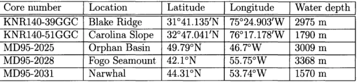
3-3 Age model for core MD95-2025 from the Orphan Basin, in calibrated years before present. Data and their sources are listed in Table 3.4. A linear interpolation and extrapolation was used to determine ages for each sample used for alkenone measurement .. .. ... 44

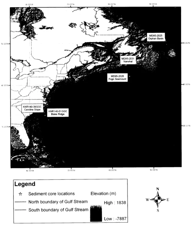
4-1 Map of the northwest Atlantic highlighting sediment core locations. Sediment core locations are listed in Table 3.1. Contour lines show 0 nm, 500 m, 1000 in, 2000 in, and 3000 in below mean sea level. Gulf Stream boundaries shown delineate the la (68.3%) confidence interval of the Gulf Stream position determined from satellite data [24]. . . . 46 4-2 Values of alkenone unsaturation parameter UIk and combined

concen-tration of C37:2 and C3 7:3 alkenones in core KNR140-39GGC from the

Blake Ridge... . ... . ... . 48

4-3 Alkenone-based sea surface temperatures for core KNR140-39GGC from the Blake Ridge. The modern sea surface temperature is from the LEVITUS94 dataset [25]. The age model used in lower panel is shown in Figure 3-1. ... ... 49

4-4 Values of alkenone unsaturation parameter U37 and combined concen-tration of C37:2 and C37:3 alkenones in core KNR140-51GGC from the

4-5 Alkenone-based sea surface temperatures for core KNR140-51GGC from the Carolina Slope. The modern sea surface temperature is from the LEVITUS94 dataset [25]. The age model used in lower panel is shown in Figure 3-2. . ... . ... ... 52 4-6 Values of alkenone unsaturation parameter U37 and combined

concen-tration of C37:2 and C3 7:3 alkenones in core MD95-2028 from the Fogo

Seamount... ... 55

4-7 Alkenone-based sea surface temperatures for core MD95-2028 from the Fogo Searnount. The modern sea surface temperature is from the LEV-ITUS94 dataset [25]. . ... ... . . 56 4-8 Values of alkenone unsaturation parameter Uk' and combined

concen-tration of C37:2 and C3 7:3 alkenones in core MD95-2031 from Narwhal. 59 4-9 Alkenone-based sea surface temperatures for core MD95-2031 from

Narwhal. The modern sea surface temperature is from the LEVITUS94

dataset [25]... . ... ... 60

4-10 Values of alkenone unsaturation parameter Uk' and combined concen-tration of C37:2 and C37:3 alkenones in core MD95-2025 from the Orphan

Basin ... ... . . . . 64

4-11 Alkenone-based sea surface temperatures for core MD95-2025 from the Orphan Basin. The modern sea surface temperature is from the LEV-ITUS94 dataset [25]. The age model used in lower panel is shown in

Figure ??... ... 65

5-1 Map indicating locations of alkenone temperature data in the slope water region. Locations with green labels are from this study; pink labels indicate study sites of Sachs et al., 2006 [44]. ... 71 5-2 Slope water temperature data from this study and from Sachs et al.,

5-3 Alkenone-based sea surface temperatures (this study) and 6180 mea-surements from G. sacculifer [23]. Scales of sea surface temperature

and 6180 are aligned to be equivalent according the Craig, 1965 [8]

modification of the Epstein et al., 1953 [13] calibration, assuming that the oxygen isotope composition of seawater is 0%o. This assumption is roughly accurate for the late Holocene, but provides a bias toward lower temperature in the early Holocene, when global ice volume was greater and mean 618() of sea water was thus higher. The modern sea surface temperature is from the LEVITUS94 dataset [25]. The age

model used in the lower panel is shown in Figure 3-2. .... ... . 73 5-4 Insolation variations over the Holocene. Parameters shown are (a)

Precession parameter, (b) obliquity, (c) summer solstice insolation at 650N and (d) annual mean insolation at 650_{N. From Crucifix et al.,}

List of Tables

3.1 Sediment cores used in this study. ...

...

32

3.2 Samples where overlapping GC peaks in the initial analysis interfered

with alkenone quantitation and necessitated saponification. . a ....

35

3.3 Planktonic foraminifera samples submitted to NOSAMS for dating. .

40

3.4 Age model data for MD95-2025, Orphan Basin. . ...

43

4.1 Alkenone data from KNR140-39GGC, Blake Ridge. Depth shown is

the mean depth of a 1-cm-wide slice. Temperature was calculated

according to Equation 3.2 from Prahl et al., 1988 [39]. Unsaturated

alkenone concentration is the sum of C

37

:

2

and C

37:3

concentrations, in

nanograms of alkenone per gram dry weight of sediment. ...

.

50

4.2 Alkenone data from KNR140-51GGC, Carolina Slope. Depth shown

is the mean depth of a 1-cm-wide slice. Temperature was calculated

according to Equation 3.2 from Prahl et al., 1988 [39]. Unsaturated

alkenone concentration is the sum of C

37

:

2

and C

3 7

:

3

concentrations, in

nanograms of alkenone per gram dry weight, of sediment. . ...

.

53

4.3 Alkenone data for MD95-2028, Fogo Seamount. Depth shown is the

mean depth of a 1-cm-wide slice. Temperature was calculated

ac-cording to Equation 3.2 from Prahl et al., 1988 [39]. Unsaturated

alkenone concentration is the sum of C

37

:

2

and C

3 7

:

3

concentrations, in

4.4 Alkenone data for MD95-2031, Narwhal. Depth shown is the mean depth of a 1-cm-wide slice. Temperature was calculated according to Equation 3.2 from Prahl et al., 1988 [39]. Unsaturated alkenone con-centration is the sum of C37:2 and C3 7:3 concentrations, in nanograms

of alkenone per gram dry weight of sediment. This dataset is continued in Table 4.5 ... . ... . . . . . ... .. 61 4.5 Alkenone data for MD95-2031, Narwhal, continued from Table 4.4.

Depth shown is the mean depth of a 1-cm-wide slice. Temperature was calculated according to Equation 3.2 from Prahl et al., 1988 [39]. Unsaturated alkenone concentration is the sum of C3 7:2 and C37:3

con-centrations, in nanograms of alkenone per gram dry weight of sediment. 62 4.6 Alkenone data for MD95-2025, Orphan Basin. Depth shown is the

mean depth of a 1-cm-wide slice. Temperature was calculated ac-cording to Equation 3.2 from Prahl et al., 1988 [39]. Unsaturated alkenone concentration is the sum of C37:2 and C3 7::3 concentrations, in

nanograms of alkenone per gram dry weight of sediment . . ... . 66 5.1 Modern mean annual, February, and August sea surface temperatures

at the locations of sediment cores used in this study. Data are from the LEVITUS94 database [25]. Core sites are listed in order of increasing

Chapter 1

Introduction

In the context of a 65 million year record of global climate fluctuations [53], the current interglacial period, known as the Holocene, is thought to be a. period of fairly stable climate [15]. With the exception of an abrupt transition to colder temperatures at around 8200 years before present (B.P.) [2], Holocene temperatures reconstructed from oxygen isotopes in Greenland ice cores appear to have remained almost constant, in contrast to the glacial-interglacial cycles of the previous 250,000 years [10].

Recent studies of sea surface temperatures in the northwest Atlantic based on alkenone unsaturation ratios have indicated that ocean temperatures decreased by about 100C over the Holocene [21]. This result is surprising, and seemingly at odds with the previous understanding of Holocene temperatures [10]. Though there has been some previous alkenone evidence of a modest. cooling of 1 - 30C, those data ap-parently conflicted with oxygen isotope and species abundance data from planktonic foraminifera from the same sites that showed no cooling trend [27].

The monotonic decrease in sea surface temperature seen in alkenone data from the Laurentian Fan is not undisputed by evidence from foraminiferal oxygen isotopes [21], and a clear climatic mechanism for such a cooling is not obvious. These uncertainties in the interpretation of Laurentian Fan alkenone data prompted a need for additional data.

In order to examine the timing and extent of the apparent. surface ocean cooling over the Holocene, we selected several sites in the slope water region of the

north-western Atlantic for further alkenone-based analysis. The alkenone technique relies on measuring the relative proportions of several specific unsaturated methyl ketones, compounds produced in the mixed layer of the ocean by coccolithophorids, a type of phytoplankton. The alkenone unsaturation parameter U" has been previously established as a proxy for mean annual sea, surface temperature in numerous stud-ies [37, 39, 46, 29].

This thesis begins with a review of the alkenone unsaturation parameter Uk' and its use as a proxy for sea surface temperature. A review of current understanding of Holocene climate follows. A section describing the oceanography and climate of the slope water region places the study sites in a geographic and climatic context. Sections describing analytical methods used and results obtained in this study follow the review sections. We conclude with discussion of possible explanations for the ap-parent Holocene cooling in slope waters substantiated by the alkenone data presented here.

Chapter 2

Background: Holocene climate and

oceanography of the North

Atlantic and Alkenone

Paleothermometry

2.1

Holocene Climate of the North Atlantic

2.1.1

Proxy records

Many paleoceanographic proxies have been used to decipher the history of climate during the Holocene, or roughly the last 10,000 years. An early indication from the O80 in Greenland ice seemed to indicate that climate, or more specifically air temperature over Greenland, had been quite stable over the Holocene, particularly compared to the magnitude of variability during glacial periods [15, 10].

The only apparent Holocene climate fluctuation of any significance in Greenland is the 8.2 kyr cold event [2]. At this time, methane concentration, accumulation rate, and 61`0 of the ice all decreased and salt concentrations in the ice increased. These changes indicate a drier and dustier period approximately 50_{C colder over} Greenland that lasted several hundred years [2]. Evidence from the slope water region

in the western north Atlantic indicate that ocean temperatures there may have been suppressed around that time for as long as 700 years [21]. Although the effects of this event on atmosphere and ocean temperatures seem prolonged, the cause is now thought to have been a quick release of about 5 Sv (1 Sv = 106 m3/s) of flood water from glacial Lake Agassiz lasting less than a year [7] .

The high resolution record of CO2 in ice from Siple Dome, Antarctica,

demon-strates that CO2, an important "greenhouse gas", was not constant over the Holocene [1]. The compilation by Ahn and coworkers [1] of that CO2 data, with other previously

published data from various Antarctic ice cores provides a good picture of how several important climate variables covaried, and that figure is reproduced as Figure 2-1 here. Evidence for sea. surface temperature variations comes from many locations in the north Atlantic area. Hald et al. [16] report foraminiferal assemblage data that indicate that slope SSTs in the Norwegian Sea near Svalbard increased during the earliest Holocene (approximately 10,800 cal. years BP according to radiocarbon dating) by about. 3 - _{4VC, remained at that higher temperature until about 8800 cal. years BP,}

and then decreased again.

Marchal and coworkers [27] provided a statistically rigorous examination of ocean temperature evidence from multiple proxies. They found that alkenone-based sea surface temperature records from seven locations around the northeast Atlantic and Mediterranean all show a statistically significant. cooling over the Holocene. However, that result stood in sharp contrast to evidence they examined from foraminiferal

O180

and foraminiferal abundance data, which show no clear temperature trend. Diatom assemblages from several of their cores indicate a possible cooling of up to 5oC over the period, but neither the timing nor magnitude of the diatom reconstruction agrees with the alkenone evidence, where they occur in the same core. Though the statistical tests of Marchal and coworkers [27] demonstrate the fidelity of trends in the alkenone data, they also demonstrate the significance of a lack of trend in the foraminifera data.

Another compilation of alkenone-based SST records by Lorenz and coworkers [26] also found a general pattern of surface cooling over the middle and late Holocene in

300 290 280 270 260

250

240 230 220 210 200 190 180 0 2 Figure 2-1: CO2 al., 2004 [1]. -180 -190 -200 -210

-220

-230

-240

-250

-270' -280 -290 4 6 8 10 12 14 16 18 20 22 24 26 28 30 32 34 36 38 40

GISP2 age (kyrBP)

the extratropics.

2.1.2

Modeling studies

Several models of Holocene climate have also indicated significant variation in ocean temperature over this period.

Renssen et al. [41] employed a coupled model including atmosphere, ocean, sea ice, and vegetation to simulate variation in atmosphere and ocean circulation and changes in sea surface temperature during the Holocene. The model included realistic insolation and prescribed methane and carbon dioxide concentrations estimated from Raynaud et al. [40]. The modeled temperature decrease in high northern latitudes of 20_{C over the Holocene is broadly consistent with proxy data.}

Lorenz and coworkers [26] explored temperature trends over the past 7000 years in order to understand the alkenone temperature data they had compiled. Their model results indicated a mean warming of the northwest Atlantic near the Grand Banks of approximately 1'C, and no clear trend in the slope water south of that region. However, they calculated a decrease in summer temperature and increase in winter temperature in the same area that is consistent with the lower insolation contrast between summer and winter at Northern mid-latitudes in the early Holocene.

2.2

Oceanographic setting and climatology of the

slope water region

2.2.1

Surface currents

The dominant oceanographic feature in the surface northwest Atlantic is the Gulf Stream. Warm waters of the Caribbean Current pass through the Florida Straits, join up with the Antilles Current, and then continue up the coast of the U.S. as the Gulf Stream, closely following the edge of the continental shelf. The Gulf Stream then separates from the coast by Cape Hatteras and heads out into the open ocean. From that point, the path of the Gulf Stream is highly variable, and a considerable

number of Gulf Stream meanders separate off into eddies known as "cold core rings" and "warm core rings" if they move south or north from the Stream, respectively. A coordinated survey in 1950 employed several U.S. Navy and research vessels to observe the Gulf Stream in a coordinated way, and one key result was confirmation that the eddies form when large amplitude meanders in the Gulf Stream close off [14]. A statistical study of satellite observations found that at least 24% of Gulf Stream crests (meanders to the north of the mean path) separate off to form warm core rings. These warm core rings are particularly important to the slope water region between the Gulf Stream and the continental shelf, because the eddies transport anomalously

warm and salty water northward.

In addition to mesoscale eddies coming off of the Gulf Stream, the slope water is influenced by additional currents, particularly the Labrador Current and a so-called "slopewater current [14]." The slopewater current flows eastward through the slope water region after splitting off from the Gulf Stream [33], and the Labrador Current

flows _{south and westward from the Labrador Sea and loops around the Grand Banks.}

The Labrador Current cools and freshens the northwest Atlantic slope waters. A map illustrating the surface currents in the slope water region is shown in Figure 2-2, from

Pickart et al., 1999 [33].

2.2.2

The Gulf Stream separation

From the first attempts to write down a set of governing equations (e.g. l\Munk, 1950 [30]) to more recent and more complicated modelling efforts, many oceanogra-phliers have sought to understand what controls the mean circulation and variability in the northern Atlantic Ocean. Even a simple model of a rectangular basin where the Coriolis parameter _{varies with latitude is sufficient to explain the need for}

western-intensification of the overall surface gyre circulation in the northern Atlantic [47]. However, models and modellers still disagree over what controls the separation of

the _{Gulf Stream from the coast at Cape Hatteras. Indeed, many models are unable to}

simulate the observed separation of the Gulf Stream, even in the presence of realistic bottom topography. Numerous hypotheses about the mechanism of Gulf Stream

65 W (60 W

56 r Figure 2-2: Surface currents in

m, 2000 m, 3000 in, 4000 m, 1999 [33].

the slope water region. Contours show 200 m, 1000

and 5000 m depth. Reproduced from Pickart et al.,

50 \ 45 N 4'i N 50 N 4• N 3• N 45 5 SC W 45 VW .. 0 W '-ýb W 50 W

separation are still being debated. One of the first hypotheses proposed was that the western boundary current separates from the coast at the latitude of zero wind curl [30]. Another prominent idea is that separation is due to interaction between the surface Gulf Stream and the Deep Western Boundary Current [50]. Another possibility, that separation is controlled by the joint effect of baroclinicity and relief (JEBAR), relies on contribution of density stratification and non-negligible bottom topography to the overall vorticity budget to explain the seaward bend in the Gulf Stream's path (see e.g. Myers et al., 1996 [31]). The mechanism of Gulf Stream separation is an outstanding problem in physical oceanography, and the possibility that the separation point may have differed under different climatological conditions bears further exploration.

2.2.3

The slope water

A compilation of hydrographic data from the slope water region revealed some signif-icant patterns of circulation and variability [33]. As Fuglister and Worthington [14] initially identified, the slopewater current, is observed as a jet unique from the Gulf Stream. Using an empirical orthogonal function (EOF) analysis of a series of hy-drographic sections at either 50 or 55°W, Pickart et al. [33] found that in the slope water region, the slopewater jet and Labrador Current either strengthen or weaken in concert. In their strengthened state, the slopewater jet moves onshore. The deep circulation in these sites seems to covary with the surface flows as well. During times of strengthened surface currents, the flow at greatest depth, the southward-flowing Denmark Strait Overflow Water, is also strengthened relative to its mean. In contrast, the mid-level flow of the Labrador Sea Water is weakened.

A recent. study by Dupont et al. [12] analyzed the heat, volume and salt budgets in the slope water region using results from a high-resolution ocean circulation model. Their primary conclusion is that properties in the slope water area. are set by influences from the Gulf Stream, Slope Water Current, and Labrador Current, and by fluxes of heat from sea surface to atmosphere. They implied that under a slightly warmer climate, the formation of Slope Water would be decreased and the region would be

more strongly influenced by Gulf Stream properties.

2.2.4

Climatology: the North Atlantic Oscilation

The dominant climatological feature in the North Atlantic on interannual to decadal time-scales is the North Atlantic Oscillation (NAO). Similar to the better-known El Nifio - Southern Oscillation (ENSO), the NAO is a coupled oscillation in the ocean and atmosphere. In the positive phase of the NAO, atmospheric pressure is higher over the Azores and lower over Iceland, compared to the mean. A positive NAO index is correlated with slightly increased sea surface temperature in the slope water region [28].

2.3

Alkenone unsaturation ratio as a sea surface

temperature proxy

The use of alkenone unsaturation ratios as a proxy for sea surface temperature (SST) has recently gained broad application in the paleoceanography field. Volkman et al. [52] first reported the existence of the C37 - C3 9 methyl and ethyl ketones with

two or three double bonds that later became commonly referred to as "alkenones." An initial study by Brassell et al. [6] showed that the degree of unsaturation in long-chain ketones produced by certain coccolithophorids was related to growth temper-ature. Since then, many workers have cultured the haptophyte algae which produce unsaturated C37 alkenones to establish the specific temperature (e.g. [37, 39])

nutri-ent [51, 38], and light [51, 38] dependence of the unsaturation patterns.

Core-top calibration studies [39, 45, 42, 29] have compared the alkenone un-saturation ratios of material extracted from sediments to the seasonal and annual sea surface temperature of overlying waters. Studies of alkenones extracted from near-surface seawater offer snapshots of water-column alkenone inventories that are difficult to compare with core-top studies, which examine alkenones produced over a much longer time period. Nonetheless, studies of alkenones in seawater particulate

organic matter provide additional information about the total amount and relative

proportions of different alkenone compounds produced under a range of ocean

con-ditions [4, 36, 34]. When comparing alkenone studies, it is important to differentiate

between the source of the measured alkenones (e.g. core-top sediments, algal culture,

or seawater) and the parameters to which they are being compared (e.g. seasonal or

annual average sea surface temperature, culture growth temperature, or instantaneous

sea surface temperature.)

2.3.1

Calibration of UP as a temperature proxy

The first calibration between alkenone unsaturation ratios and temperature came

from Brassell et al. [6], who introduced the use of the U~7 index, which is defined as

[C37:2] - [C3 7:4]

[

37 -C37:2]+ [C3 7:3] [C37:4]

where [C37:2], [C:37.3], and [C37:4] represent concentrations of di-, tri-, and

tetra-unsaturated C

37

methyl ketones respectively. These three compounds, whose

struc-tures are shown in Figure 2-3, have been identified as

(E,E)-15,22-heptatriacontadien-2-one, (E,E,E)-8,15,22-heptatriacontatrien-(E,E)-15,22-heptatriacontadien-2-one, and

(E,E,E,E)-8,15,22,29-heptatriatetraen-2-one by several groups [11, 52].

Prahl and Wakeham [37] first introduced the use of U"7

,

which differs from the

U~

7

index only in the neglect of the tetra-unsaturated C

37

methyl ketone. Specifically,

the U17 index is defined as

Sk'

C37:2

37

_C37:2

37 2 C37 3 (2.2)

+ C37:3

One commonly-used calibration between Uk7 comes from a core-top study by

Miiller et al. [29]. By comparing core-top values of U7 fromr over a hundred samples

with mean annual. production-weighted annual, and seasonal temperatures, they

de-termined that the best fit between Uk7 and temperature comes from using the mean

annual sea surface temperatures of overlying water.

2.3.2

Seasonality of alkenone production and

Uk

The issue of whether alkenones in surface sediments reflect the overlying water

tem-perature is already implicit in calibration studies. That is, the relationship between

the U37 index and sea surface temperature was defined to provide the maximum

pos-sible correlation between these two properties, and that maximum correlation was

found between U"; and mean annual surface temperature for the popular calibration

determined by Miiller et al. [29].

The same study also compared U" with mean

annual temperature at a variety of depths, production-weighted annual mean

sur-face temperature, and seasonal average sursur-face temperature, all of which had lower

correlation coefficients than mean annual temperature at the surface.

Prahl and coworkers [36] measured alkenone production and composition in

partic-ulate organic matter and from sediment traps at Station ALOHA in the oligotrophic

North Pacific. They determined that alkenone production and export events can

take place in both winter and summer, for separate reasons. They linked the

sum-mer export events to "new production" caused by nitrogen fixation in the surface

mixed layer, whereas the winter events were tied to eddy-scale mixing of nutrients

up from deep waters and occurred in the deep chlorophyll maximum layer. Even

though the winter export events occurred deeper in the water column and at a colder

temperature, U3' values representing a production-weighted average of summer and

winter export were in agreement with mean annual sea surface temperatures. Prahl et

al. therefore concluded that the seasonality of alkenone production and longer-term

variations in ecology and productivity should not affect the applicability of U3 as a

paleoclimate proxy.

2.3.3

Preservation of alkenone signal

In order to have confidence in a paleo-temperature reconstruction based on alkenone

unsaturation ratios, we need to be confidant that the unsaturation pattern measured

from a sediment core sample is not substantially different from the alkenone

unsatu-ration ratio in the overlying water column at the time that sediment was deposited.

Sikes et al.

[45]

provide some evidence that U3L values do not change during routine handling and storage procedures typical for sediment cores designated for paleoceano-graphic studies, at least over storage periods up to four years. Thus if the signal has not been altered in the water column or sediments prior to core collection, an authen-tic Utk value can be measured.

There are several questions to answer in addressing the issue of whether sedimen-tary U"' specifically represents the temperature of overlying waters at the time the sediment was deposited. First, does the Uk of lipids extracted from surface sediments record the same signal as the overlying water? How does sediment redistribution af-fect. alkenone deposition? And finally, do early diagenetic processes, and particularly oxidative degradation, alter the U37 composition of down-core sediments?

Prahl et al. [35] investigated preservation of alkenones in marine sediments by comparing sediment from above and below an oxidation horizon in two different cores from the same massive turbidite deposit. They found that although the concentration of alkenones in the sediments decreased by about 88% from the unoxidized to the oxidized section of the turbidite, the Ul values were very similar. When translated to temperature using the calibration by Prahl et al., 1988 [39], the variation of Uk'

values between oxidized and unoxidized samples corresponds to less than P1C. These results suggest that the U 37of sediments is not altered by exposure to oxygen (and by implication also nitrate and other weaker oxidizing agents.) Investigating the effect of carbonate dissolution on U37, Sikes et al. [45] found that exposure of sediments to acidic conditions in a laboratory setting did not affect U3' values, even when the exposure to acid was sufficient to dissolve almost all carbonate from a moderately carbonate-rich sediment. They additionally noted that offsets between U37-based

SST from core-top samples and measured SST of overlying waters in a global dataset were not correlated with water depth, so Sikes et al. [45] concluded that carbonate dissolution does not impact Uk7.

2.3.4

The imperfect relationship between U37 and SST

Not all studies have shown U" to be linearly well-correlated to mean annual sea surface temperature, particularly at low temperatures and low salinities. Some stud-ies [4, 42] suggest that U37 is much better correlated than U" to sea surface tem-peratures when those temtem-peratures are low, particularly below about 80 C. Other work [46] has demonstrated that U3k can still correlate well with the low tempera-tures characteristic of the Southern Ocean, and that U3 is a better proxy than Uk7 for temperature in the Southern Ocean. A comparison between core-top Uk7 and

U37 values at high northern and southern latitudes [42] showed that although Uk correlates well with SST in both hemispheres, the exact relationship differs between the Southern Ocean dataset and the Nordic Seas dataset. Uk', on the other hand, did not show the same relationship to SST in the high northern latitudes as it had in the high southern latitudes [42]. Sites where Bendle and Rosell-Mel6 [4] demon-strated U37 and SST pairings inconsistent with the Mfiller et al., 1998 [29] calibration occurred almost exclusively north of 670

N in the Nordic Seas, so the Miiller et al., 1998 [29] calibration should still be applicable in regions south of 67'N. The break-down in a linear relationship between Uk7 and SST at low temperatures thus seems geographically constrained, though it does provide reason for caution when applying the proxy into the past.

Salinity also may have a significant effect on U37 [5], at least at the lower salin-ities of coastal waters. A study of alkenone production and unsaturation patterns across a salinity transect between the North Sea. and the Baltic Sea showed that even though temperature, light, and nutrients were almost constant over the region, U3k

varied significantly, and was correlated to sea surface salinity [5]. These results came from measuring both particulate organic matter from a bloom of E. huxleyi, a major alkenone-producing species, and alkenones extracted from surface sediments. They were able to rule out significant contributions of sedimentary alkenones from other species based on the patterns of alkenone and alkenoate compounds, so the unex-pected lack of a clear relationship between U'7 and SST could not be attributed to

an unknown alkenone producer.

In a culture study of the somewhat uncommon alkenone-producing species

Isochry-sis galbana, Versteegh and coworkers [51] determined that U37 values can be altered by

both nutrient and light limitation, producing an apparent temperature offset around 2-3'C. Prahl and coworkers [38] cultured the ubiquitous Emiliania huxleyi and also determined that nutrient limitation causes Uk' values to be too low for the given

/

0-Figure 2-3: Chemical U37 and U3. /-,4 CIA

U

Q) CO

I

Z

I

Z

a) · (.-o4 G, c(5 6"=

/

/

0

/

/

0

Chapter 3

Methods

3.1

Samples

Samples for alkenone analysis were collected from five available sediment cores. The gravity core 51GGC was collected from the Carolina Slope (32'47.041'N, 76017.178'W) at 1790 m water depth on R/V Knorr Cruise 140 Leg 2 during November, 1993. On the same cruise, gravity core 39GGC was collected from the Blake Ridge (31'40.135'N, 750_{24.903'W) at 2975 m water depth. Core 51GGC and 39GGC were sampled every} 4 cm to a total depth of 2.9 m in core 51GGC and 1.17 m in core 39GGC. Three cores from the Marion Dufresne cruise MD101, part of the IMAGES program, were also sampled. Core MD95-2025 comes from the Orphan Basin (49.79'N, 46.70_W)

at 3009 m water depth. The archive section of the Orphan Basin core was sampled every 100 cm over the top 30 m of core. Core MD95-2028 was collected from the Fogo Seamount (42.10_{N, 55.75}0_{W) in 3368 in of water. The archive section of the Fogo} Seamount core was sampled every 100 cm for the first 5 m of core, every 200 cm to a depth of 19 in, and then every 100 cm again to a final depth of 22 m. Core MD95-2031 comes from a site in the Grand Banks called Narwhal (44.31'N, 53.74'W) in 1570 m of water. The Narwhal core was sampled every 20 cm from the coretop down to a maximum depth of 12 m.

Samples were taken from a 1 cm depth interval, and ca.re was taken to exclude material that had touched the sides of the core liner and material that had been

Core number Location Latitude Longitude Water depth KNR140-39GGC Blake Ridge 31041.135'N 75024.903'W 2975 m KNR140-51GGC Carolina Slope 32047.041'N 76017.178'W 1790 m

MD95-2025 Orphan Basin 49.79°N 46.70W 3009 m

MD95-2028 Fogo Seamount 42.1°N 55.75oW 3368 m

MD95-2031 Narwhal 44.31oN 53.740_{W 1570 m}

Table 3.1: Sediment cores used in this study.

exposed to the air after the core had been split. Each sample represented between 5 g and 15 g wet mass. Samples were stored frozen at -20 to -30'C in precombusted 16 ml glass vials, and then freeze-dried at -500C using a Virtis Benchtop freeze-drier for several days, after which they were stored in a dessicator prior to lipid extraction.

3.2

Lipid Extraction

All materials were pre-combusted at 4500C or greater for at least 8 hours. All tools and equipment, including the stainless steel cells, were washed with tap water (3x) and deionized water (3x), and then either sonicated in methanol and then dichloromethane (DCM) for at least 3 minutes each, or rinsed sequentially in methanol (3x), DCM (3x), and hexanes (3x). For extraction of each sample, first 3-5 g of pre-combusted Na2SO4 and then 3-12 g of dry, ground-up sediment. was loaded into a stainless

steel cell with a similar mass of Na2SO4 and 20 pl of 0.103mg/ml n-C3 7 alkane in

toluene internal recovery standard, glass fiber filters (VWR®, pore size 1.5 pim) on either end of the cell, and quartz sand (Accusand®) separated by another filter to fill the cell. Samples were then extracted with DCM using a DIONEX ASE 200 Accelerated Solvent Extractor. Each sample was extracted using 3 consecutive 5-minute extraction cycles at 1500 psi and 1500C. A slightly modified procedure was used to extract samples that needed to be preserved for future isotopic work on foraminifera. For these samples (roughly half of the samples from MD95-2025 and MD95-2031, and all samples from MD95-2028), the sediment was gently mixed with a spatula rather than ground, and Na2SO4 on either side of the sample was separated

by a glass fiber filter. These samples were extracted in the ASE at 1000 psi and 1000C.

After extraction, all samples were dried down under nitrogen using a Zymark TurboVap evaporator and stored at -20 to -300C, if necessary. Total lipid extracts were then transferred to 2 ml borosilicate Target® vials (National Scientific®) using rinses of acetone/DCM (1:1 v:v), DCM (2x) and hexanes, and solvents were evaporated under nitrogen. Total lipid extracts were dissolved in 400 pl toluene with a known quantity of n-C36 alkane quantitation standard and derivatized by silylation with 10 pl bis(trimethylsilyl)trifluoroacetanide (BSTFA) at 500C for one hour using a Pierce Reacti-Therm IIITM _{hot plate in preparation for alkenone identification and} quantification by gas chromatography.

3.3

Alkenone Quantitation

Di- and tri-unsaturated C3 7 alkenones were identified and quantified using an Agilent

Technologies 6890N gas chromatograph with flame ionization detection (GC-FID). A 10 pl aliquot of the 410 pl derivatized total lipid extract solution was injected onto the 60-m-long, 0.32 mm diameter fused silica Chrompack capillary column (CP-Sil 5CB, #CP8744) using a 7683 Series injector with autosampler. Identification of n-alkane standards and alkenone peaks was made by comparison of retention time with a known sediment standard. Determination of alkenone concentrations was achieved by comparison of alkenone peak areas with the area of the n-C:₃₆ alkane quantitation standard.

Some samples, particularly from core MD95-2025, had very low alkenone con-centrations, such that a 10 pl aliquot out of 410 pl of total lipid extract solution was insufficient to robustly determine the alkenone concentrations. After the initial quantitation and determination of low concentration, these samples were dried down under nitrogen and then re-derivatized with 2 pl BSTFA in either 20 or 40 pl of dry toluene at. 500C for one hour. A 10 pl aliquot of the 22 or 42 I1 solution was then injected on the GC-FID for alkenone quantitation.

3.4

Saponification

A number of samples, particularly some with low alkenone concentrations, contained compounds whose peaks overlapped with those of the two C37 alkenones being

mea-sured, such that alkenone quantitation was not initially possible. Since the interfering compounds were suspected to be primarily fatty acids and alcohols with more polar moieties than the alkenone compounds of interest, those sample were hydrolyzed to separate the ketones for additional analysis.

The total lipid extracts were dissolved in 3 ml of 1N KOH in methanol and son-icated for approximately 3-4 minutes. After that, 1 ml of dichloromethane- (DCM-) extracted deionized water was added and the samples were shaken vigorously. The vials were then capped under nitrogen and allowed to sit in an oven at 600C overnight in order for the hydrolysis reaction to proceed fully.

The polar and non-polar compounds were then separated by adding approximately 15 ml each of DCM-extracted water and hexane to the solutions. The solution was shaken vigorously and then the solvents were allowed to separate. The hexane frac-tion, containing the less polar compounds, was then carefully pipetted off into a separate vial. An additional 15 ml of hexanes was added 3 more times and the pro-cess repeated. The aqueous fraction, containing the more polar compounds, was saved separately.

The hexane fraction was then back-extracted using 15 ml DCM-extracted water. After vigorous shaking and subsequent settling and separation of the solvents, the hexane portion was carefully pipetted off into a new vial containing a small amount of pre-combusted sodium sulfate (Na2SO4), to remove any remaining water. The

hexane was finally transferred to one last clean vial, and the sodium sulfate was rinsed 3 times with several milliliters of clean hexane.

The hexane fraction was finally dried down under nitrogen, then transferred to a small GC vial and re-derivatized with BSTFA, as above, for analysis by GC-FID. Samples that needed saponification are listed in T'able 3.2.

Core number

Location

Depth

MD95-2025 Orphan Basin 300-301 cm MD95-2025 Orphan Basin 400-401 cm MD95-2025 Orphan Basin 600-601 cm MD95-2025 Orphan Basin 1000-1001 cm MD95-2025 Orphan Basin 1800-1801 cm MD95-2025 Orphan Basin 2000-2001 cm

MD95-2025 Orphan Basin 2100-2101 cim

MD95-2025 Orphan Basin 2200-2201 cm

MD95-2025 Orphan Basin 2900-2901 cm

MD95-2028 Fogo Seamount 1100-1101 cm

MD95-2031 Narwhal 1080-1081 cm

Table 3.2: Samples where overlapping GC peaks in the initial analysis alkenone quantitation and necessitated saponification.

interfered with

3.5

Standards

Standard solutions were used to quantify alkenone concentrations and to measure loss of the total lipid extract during transfers and processing. The internal recovery

standard solution used was 0.103 ing/ml n-C37 alkane in toluene. The quantitation

standard used was 5.122 pg/nml n-C36 alkane in toluene.

To measure procedural precision, a sediment standard from Bermuda Rise core GGC-5 (referred to as BRC) was measured after approximately every 10 samples. Overall precision in measuring U37 from the BRC standard was 0.0256 in U<7 units, which is equivalent to 0.75°C, or less than the standard error for reconstructing tem-perature using a number of core-top calibrations [29]. Reproducibility of the alkenone concentration was ±10% of the concentration measured.

3.6

Calculation of U

7

The parameter UJ7, defined in Equation 2.2, was calculated as the ratio of con-centrations of the two methyl ketone compounds. An alkenone-based sea surface

temperature was then calculated from the U/ according to: U3 = 0.039 + 0.034 * T (3.1) or alternatively, U_{k' - 0.039} T = -0.039 _(3.2) 0.034

from the E. huxleyi culture calibration of Prahl et al., 1988 [39].

3.7

Age Models

3.7.1

Blake Ridge, KNR140-39GGC

For core KNR140-39GGC, calibrated 14C dates from planktonic foraminifera were provided by L. Keigwin (pers. comm.) as published by Keigwin and Schlegel [22]. Original radiocarbon dates were calibrated according to Stuiver et al., 1998 [48] and Bard et al., 1998 [3] by Keigwin and Schlegel, 2002 [22]. The provided dates were interpolated to the depths of alkenone measurements using the PCHIP (Piecewise-Cubic Hermite Interpolating Program) cubic spline in MATLAB to obtain the age model for that core. The age model for KNR150-39GGC is shown in Figure 3-1.

3.7.2

Carolina Slope, KNR140-51GGC

14_{C dates from planktonic foraminifera in core KNR140-51GGC [23] were calibrated}

using the CALIB v. 5.0 program [49] and the Marine04 calibration [18], which assumes a 400 year offset between marine and atmospheric carbon. No core-top date was available, so a date of 0 years BP was assumed, and the dates were then interpolated to sample depths using a linear interpolation. The age model for core KNR140-51GGC is shown in Figure 3-2.

LUUUU 15000 0-a 10000 o 5000 n

Age Model for Blake Ridge, KNR140-39GGC

0 50 100 150 200 250 300 350 400 450

Core depth, cm

Figure 3-1: Age model for core KNR140-39GGC from the Blake Ridge in calibrated years before present. The age model used in this study was interpolated from the available radiocarbon-based dates using a PCHIP (Piecewise-Cubic Hermite Interpo-lating Program) spline in MATLAB. Radiocarbon dates are from foraminifera, and calibrated ages were calculated according to Stuiver et al., 1998 [48] and Bard et al., 1998 [3] by Keigwin and Schlegel, 2002 [22]. Data courtesy L. Keigwin, 2005 (pers. CO111111.) - I I I I I 0 S S S 0 S S S S I I I I I ^^^^^""""`

Age Model for Carolina Slope, KNR140-51GGC

50 100 150 200

Core depth, cm

250 300 350

Figure 3-2: Age model for core KNR140-51GGC from the Carolina Slope in calibrated years before present. Data are from Keigwin, 2004 [23], and were converted from radiocarbon age to calibrated age using the CALIB v. 5.0 program from Stuiver et al., 2005 [49] and the Marine04 calibration dataset of Hughen et al., 2004 [18], which assumes a 400 year offset between marine and atmospheric carbon. Core-top value of 0 age is assumed, for lack of additional data. A linear interpolation was used to estimate the age-depth relationship for depths of samples.

20000 5000 10000 5000 0· ,Og · · 0 400 I I I I I ·I I t 11 nrrrnn_{Irl II} 20VV

3.7.3

MD95-2031, Narwhal

To determine an age model for this core, tests of the planktonic foraminifer G.

bul-loides were picked from the >250pmn fraction and from the 150-250ipm fraction of either extracted or non-extracted freeze-dried sediment after disaggregating and rins-ing the sample usrins-ing deionized water. Extraction at high temperature and pressure using an organic solvent has previously been shown to have no demonstrable effect on "1C content of foraminifera [32]. One sample did not have sufficient G. bulloides

for radiocarbon dating, so N. pachyderma (left-coiling) was picked from the 150-250

pmi fraction instead. After picking, the foraminiferal tests were rinsed thoroughly in deionized water and dried in an oven at approximately 500_{C. Discolored or otherwise} odd-looking tests were discarded from the samples, and care was taken to remove any non-foranminiferal material from the samples. The cleaned samples were then

submit-ted to the NOSAMS accelerator mass spectrometry facility in Woods Hole, MA for analysis. Table 3.3 lists the sample depths and species submitted. Unfortunately, age

ffi C,: C-:

S

0] 003 00s C: OO ·c3 O o0 00 00 O y y c0 C O C3 T-·I LO

I~

0b 00 00

0

0 -z C1 z C, QJ o C-40 40 vj 33 ·c; o y C o o, o J 03 C,: 0c o0 0] 0,

S

01

01

3.7.4

MD95-2028, Fogo Seamount

No age information was available for MD95-2028, and after preliminary alkenone data were obtained, it was determined that developing an age model at this site would be beyond the scope of this study.

3.7.5

MD95-2025, Orphan Basin

The age model for NID95-2025 comes from data published in Hiscott et al., 2001 [17]. The information from that reference used here includes four radiocarbon dates from mixed planktonic foraminifera, one age for an ash layer, and a depth for the Marine Isotope Stage (MIS) 5/6 transition visually estimated from a plot of S1 8_{0. The ash}

layer at 9.70 in was determined by Hiscott et al. to be the 57.5 ka Ash 2 from Ruddiinan and McIntyre, 1984 [43]. The age of the MIS 5/6 transition was taken from Imbrie et al., 1984 [20] to be 127 ky B.P. The ages of the two younger radiocarbon samples from Hiscott et al. were calibrated for this study using the CALIB v. 5.0 program from Stuiver et al., 2005 [49] and the Marine04 calibration dataset of Hughen et al., 2004 [18], which assumes a 400 year offset between marine and atmospheric carbon. The other two radiocarbon ages given were too old to use the Stuiver et al. [49] program or the Hughen et al. [18] datasets, and were left in uncalibrated radiocarbon years, for which Hiscott and coworkers [17] used a 5568 year half-life for

"

4

C and assumed no reservoir correction. Little difference was noticed in the overall age model after changing the younger two ages from radiocarbon years to calibrated years.

A core-top age of 0 years B.P. was assumed, since no age above 60 cm was given. However, a sample of G. bulloides was picked from the 0-1 cm sample taken for this study. That sample was prepared as the other foraminifera samples listed for MID95-2031 (Narwhal) and was also submitted to NOSAMS in Woods Hole for AMS dating, but unfortunately that data was not available in time for inclusion in this documnent. The specific data used in the age model for MD95-2025 are listed in Table 3.4 and are depicted in Figure 3-3. Specific ages for sample depths were determined by linear

0 0 C) 0 0_;-4 0 0 ;-4 0 ct 4-)

_b-C

0 0;-4 t Cý 4--C.) o ID 0 7: CE C'] ct 0 m E ct_k O 0 0 C] o 0 0 S 0 C'] C']_ct k O1 Go L·3 c CO] 0 -z 0 .5 S

•o

cm• 0 C'_k0 C'] C'] or cu o ;-Go C']_S 0 c z ed 0

S

S 0 C']_lrt c O U-CD Cq O C' 4-4o ©_cJ

M

Cl Lfý C) ;-4 4-t 0 0 H© ©n

Age Model for Orphan Basin, MD95-2025 S S 0 S 0 S

200

400

600

800

1000 1200

Core depth, cm 1400 1600 1800

Figure 3-3: Age model for core MD95-2025 from the Orphan Basin, in calibrated years before present. Data and their sources are listed in Table 3.4. A linear interpolation and extrapolation was used to determine ages for each sample used for alkenone measurement. 120 100 20 2000 n/ 1 - · · · · | I I I I I I I I I I I h •u " 1 -E

Chapter 4

Results

Alkenone concentration and ratio data were obtained from 5 separate sediment cores from the northwest Atlantic, listed in Table 3.1 and shown in their geographic and bathymetric context in Figure 4-1. These locations span a wide range of latitude and are generally located along the continental slope.

Alkenone-based temperatures from the two sites south of Cape Hatteras, where the Gulf Stream separates from the slope and heads out to sea, show fairly steady temperatures over the Holocene, with ranges of only a few degrees Celsius at the Blake Ridge and Carolina Slope locations. The sites farther north show considerably more variation, though it was determined through alkenone analysis and subsequent research that our samples from only one of the other three sites, Narwhal (MD95-2031), represent the Holocene portion of the core. Data from the two remaining cores, MD95-2028 (Fogo Seamount) and MD95-2025 (Orphan Basin) will nonetheless be presented and discussed here, though few conclusions can be drawn from them that are specifically relevant to the Holocene temperature problem.

4.1

KNR140-39GGC, Blake Ridge

Concentrations of both the di- and tri-unsaturated C3 7 methyl ketones from the Blake

Ridge samples were sufficient for good quantitation by GC-FID. The combined con-centration of both compounds and the U'/ values are shown in Figure 4-2. These

50 0'O') 40 O0N 100't4 K , 0 W 70 C' w U U V u vv

Legend

N

* Sediment core locations Elevation (m)

North boundary of Gulf Stream High

:

1838 W E

L

Low : -7887

Figure 4-1: Map of the northwest Atlantic highlighting sediment core locations. Sed-iment core locations are listed in Table 3.1. Contour lines show 0 m, 500 in, 1000 nm, 2000 mn, and 3000 in below mean sea. level. Gulf Stream boundaries shown delin-eate the l0 (68.3%) confidence interval of the Gulf Stream position determined from satellite data [24].

parameters are uncorrelated, with a correlation coefficient of -0.0187 that is not

sta-tistically significant.

With the exception of a few outliers, the alkenone temperatures measured from the Blake Ridge are within a 2°C range for the entire Holocene. Figure 4-3 shows the sea surface temperature record, calculated from U:k according to Equation 3.2 from Prahl et al., 1988 [39], versus both depth and age. The age model for this core was presented in Section 3.7.1. It should be recalled that age control was sparse for this section of the core, and the age model was constructed by assuming an age of 0 years B.P. for the core-top and interpolating from the calibrated age of 9175 years B.P. at 280 cmn depth.

The modern mean sea, surface temperature at this location is 23.9'C [25], which is within error of the alkenone SST nearest to core-top (the top of this core was disturbed, so a core-top sample sufficient for alkenone analysis could not be obtained). However, it should be noted that the measured modern SST is slightly higher than mean Holocene SST at this site. Additionally, since age control is poor for the upper portion of this core, a lack of perfect agreement, between modern and near-core-top

SST is not surprising.

4.2

KNR140-51GGC, Carolina Slope

Concentration of di- and tri-unsaturated alkenones and Uý from the Carolina Slope are shown in Figure 4-4. Alkenone concentrations are highest near the core-top

(ex-cept for one seemingly anomalous point around 230 cm depth), and there is no obvious

pattern _{of variation in concentration. Though there is no visually obvious relationship}

between concentration and U3k_{, the correlation coefficient between them is -0.3250,}

which is significant at the 95% confidence level.

Similar to the Blake Ridge, the alkenone temperatures from the Carolina Slope shown in Figure 4-5 have a range of about 20C over the Holocene. A clear drop in tempnleratures is evidenced by the alkenone data between 3000 and 2000 years B.P., after which the alkenone SST returns to its previous value.

n 00 v.o0 0.86 0.84 S 0.82 0.8 0.78 0 7A

KNR140-39GGC, Blake Ridge Alkenone Data

I o1 1000 800 r 0 600 8 C O 400 ( 200 u) n-_' 0 20 40 60 80 100 120 Depth (cm)

Figure 4-2: Values of alkenone unsaturation parameter Uk and combined concentra-tion of C37:2 and C3 7:3 alkenones in core KNR140-39GGC from the Blake Ridge.