Aspects of inference for the Influence Model and related graphical models

(1)

Aspects of Inference for the Influence Model and

Related Graphical Models

by

Arvind K. Jammalamadaka

B.S., University of California at Santa Barbara (2001)

Submitted to the Department of Electrical Engineering and Computer

Science

in Partial Fulfillment of the Requirements for the degree of

Master of Science in Electrical Engineering and Computer Science

at the

Massachusetts Institute of Technology

June 2004

@

Massachusetts Institute of Technology 2004. All rights reserved.

A uthor ...

...

Department of Electrical Engineering and Computer Science

May 21, 2004

Certified by ...

George C. Verghese

Professor of Electrical Engineering

Thesis Supervisor

Accepted by ..

Arthur C. Smith

Chairman, Department Committee on Graduate Students

MASSACHUSETTS INSTITUTE OF TECHNOLOGY

(2)

(3)

Aspects of Inference for the Influence Model and Related

Graphical Models

by

Arvind K. Jammalamadaka

Submitted to the Department of Electrical Engineering and Computer Science on May 21, 2004, in partial fulfillment of the

requirements for the degree of

Master of Science in Electrical Engineering and Computer Science

Abstract

The Influence Model (IM), developed with the primary motivation of describing net-work dynamics in power systems, has proved to be very useful in a variety of contexts. It consists of a directed graph of interacting sites whose Markov state transition prob-abilities depend on their present state and that of their neighbors. The major goals of this thesis are (1) to place the Influence Model in the broader framework of graphical models, such as Bayesian networks, (2) to provide and discuss a hybrid model be-tween the IM and dynamic Bayesian networks, (3) to discuss the use of inference tools available for such graphical models in the context of the IM, and (4) to provide some methods of estimating the unknown parameters that describe the IM. We hope each of these developments will enhance the use of IM as a tool for studying networked interactions.

Thesis Supervisor: George C. Verghese Title: Professor of Electrical Engineering

(4)

(5)

Dedicated to:

(6)

Acknowledgments

I would like to thank Professor George Verghese who has been a great teacher,

men-tor and supervisor for this thesis work. His encouragement, support and advice have made this work a pleasure for me.

My early interactions and discussions with Dr. Sandip Roy and Carlos

Gomez-Uribe steered me in this direction and for that I am thankful to both of them.

Finally, I would like to thank my family for their love and affection, and for en-couraging me to excel in whatever I do.

This work is supported by an AFOSR DoD URI for "Architectures for Secure and Robust Distributed Infrastructures" F49620-01-1-0365 (led by Stanford University).

(7)

List of Figures

2-1 A hidden Markov model expressed as a Bayesian network. Shaded

circles represent evidence nodes. . . . . 2-2 A POMNet graph and corresponding trellis diagram. Shaded circles

represent evidence nodes. . . . .

2-3 A "generalized" IM graph and trellis (DBN) structure. Solid lines

represent influence in the usual sense, whereas dashed lines represent same-time influence. The order for updating nodes at each time step

would be {1}, {2, 3}, {4} . . . ...

3-1 An example of a BN graph, and the nodes Shaded circles represent evidence nodes. .

relevant to target node 1.

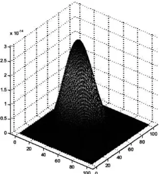
Plot of L(p, q) (p = 0.5, q = 0.5, T = 10). . . . . Estimates of p (p = 0.5, q = 0.5, T = 100). . . . . Estimates of q (p = 0.5, q = 0.5, T = 100). . . . . Estimates of p (p = 0.25, q = 0.63, T = 20). . . . . Estimates of q (p = 0.25, q = 0.63, T = 20). . . . . Plot of L(A) (p = 0.1, q = 0.4, A = 1, T = 50) .. . . . . Estimates of A (p = 0.1, q = 0.4, A = 1, T = 50). . . . .

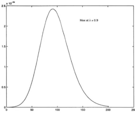
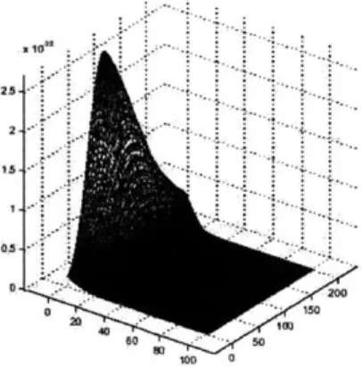
Plot of L(p, q, A), pq cross-section (p 0.1, q = 0.4, A = 1, T = 20). Plot of L(p, q, A), Ap cross-section (p = 0.1, q = 0.4, A = 1, T = 20). Plot of L(p, q, A), Aq cross-section (p = 0.1, q = 0.4, A = 1, T = 20).

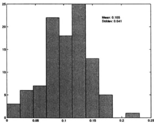
Estimates of p (p = 0.1, q = 0.4, A = 1, T = 100). . . . . Estimates of q (p = 0.1, q = 0.4, A = 1, T = 100). . . . . 22 24 25 4-1 4-2 4-3 4-4 4-5 4-6 4-7 4-8 4-9 4-10 4-11 4-12 36 47 48 49 49 50 52 52 53 53 54 54 55

(10)

(11)

Chapter 1 Introduction

Graphical models are an effective way of representing relationships between variables in a complex stochastic system. They are used in a variety of contexts, from digital communication [11] to modelling social interactions [4], and in fact have roots in sev-eral different research communities including statistics [17], artificial intelligence [23], and computational neuroscience [15].

The influence model (IM), introduced in [1] and described concisely in [2], was developed with the primary motivation of describing network dynamics in power sys-tems. It is, however, a rich stochastic model for networked components, capable of modelling systems that are complex but structured in a tractable way. It consists of a network of interacting Markov chains in a graph structure, with the next state of each chain dependent not only on its own current state, but that of its neighbors. The overall model is Markovian, in the sense that the probability distribution for the next state of the system is determined from model parameters in conjunction with the current state.

The work in [1] focuses on motivating and defining the influence model, as well as analyzing its tractability and dynamics.

(12)

mod-els called moment-linear stochastic systems, and the dynamics of those systems were analyzed, along with approaches to estimation and control.

More recently, [29] treats state estimation in the IM for cases in which we may not be able to obtain complete information about the system, by analogy with hidden Markov models. Further details regarding this approach to inference in the IM will be discussed later in this thesis.

The influence model has also been recently applied in the context of social in-teractions. In one application, it was used to model interaction dynamics among participants in a conversation

[4].

In another, it was used to model "webs of trust" in relationships between users of knowledge-sharing sites on the Internet [28].

The major goals of this thesis are: (1) to place the influence model in the broader framework of graphical models, as used in other fields mentioned above, (2) to pro-vide and discuss a hybrid between the IM and dynamic Bayesian networks, (3) to understand tools for performing efficient inference on the class of graphical models in which the influence model lies, and (4) to provide some results regarding estimation of parameters and structure for the IM.

1.1 Overview

In Chapter 2, we discuss how the IM can be embedded in the framework of graphical models. We relate it to hidden Markov models and to Bayesian networks, and provide a generalization based on this relationship. In Chapter 3, we exploit this connection to discuss algorithms for exact and approximate inference for the IM. Although we often assume the model parameters in an IM to be given, in practice, they are not. In Chapter 4, we discuss maximum likelihood estimation of these unknown model parameters. Finally, Chapter 5 provides some possibilities for potential future work.

(13)

Chapter 2 The Influence Model and Related

Graphical Models

2.1 The Influence Model

2.1.1 Definition

We first define the influence model. Consider a network which consists of n interacting nodes (or sites), evolving over discrete time k = 1, . . ., T, where node i can take on any

one of mi possible states. We denote the state of node i at time k by an mi x 1 column vector s [k] which is an indicator vector i.e., the mi-vector s2[k] contains a single 1 in

the position corresponding to the state of node i at time k, and a 0 everywhere else, for instance

s'[k] = [0 ... 010 ... 0],

where / denotes transpose.

Letting M = ET m, we denote the overall state of this networked system at

time k by the length M vector s[k], which simply consists of the collection of si [k] for

(14)

s1 [k]

s[k] = . (2.1.1)

-s, [k]

The state evolution and the network structure of the IM are governed by two things: (1) a set of state transition matrices {Aij} (where Aij is of order mi x iM)

which describe the effect of node i on node

j,

in a way analogous to the transition matrix of a Markov chain, and (2) an n x n stochastic matrix D called the "network influence matrix", whose elements dij provide the probability with which the state of node j at time k influences the state of node i in the next time step k + 1 (so d,, > 0

and Ej dij = 1). We assume that the Aij and the dij are homogeneous over time to avoid further complication.

To express the evolution of an IM, we also define pi[k], the probability vector for the next state of site i. This mi x 1 vector is defined so that the 1L" element of pi [k]

is the probability that node i is in state 1 at time k (and its entries therefore sum to

1). We also have the corresponding concatenated M-vector p[k]:

Pi [k]

p[k] = : .(2.1.2)

Pn [k]

Then, the state evolution of the IM has the following form:

pi[k + 1] =Zdi s[k]Aj. (2.1.3)

Or, more compactly,

(15)

where

dj1A ... d1An

H = i= D' @ Aij} (2.1.5)

LdinAni ... dpjnAnn

and 0 denotes the Kronecker product. The properties of the specially structured matrix H are explored in detail in [1], but are not essential to this thesis.

Some things to note: we see that si [k + 1] is conditionally independent of all other state variables at time k + 1 given s[k] i.e.,

n

P(s[k +

1]Is[k])

= JP(s[k + 1]fs[k]), (2.1.6)

i=1

and the Markov property holds for the process s[k] as it evolves over time, that is,

P(s[k + 1]js[k, s[k - 1], . - -) = P(s[k + 1]Is[k]). (2.1.7)

We also see that the influence matrix D specifies a directed graph for the structure of the model by indicating the presence or absence of dependencies between nodes.

2.1.2 An Alternate Formulation

The above way of viewing the evolution/update process makes its quasi-linear struc-ture clear, but an equivalent way of viewing the process, which might be more intuitive in certain cases, involves each site picking a "determining site" from among its neigh-bors for the update. That process can be summarized in the following three steps

(see [2]):

1. A site i randomly selects one of its neighboring sites in the network, or itself,

to be its determining site for Step 2. Site j is selected as the determining site for site i with probability dij.

(16)

s

[k].

The probability vector pi [k + 1] will be used in the next stage to choose the next status of site i, so pj[k + 1] is a length-mi row vector with nonnegative entries that sum to 1. Specifically, if site

j

is selected as the determining site, then p'[k + 1] = s'[k]Aji, where Aji is a fixed row-stochastic mj x mi matrix. That is, Aji is a matrix whose rows are probability vectors, with nonnegative entries that sum to 1.

3. The next status s [k + 1] is chosen according to the probabilities in p'[k + 1],

which were computed in the previous step.

2.1.3 Expectation Recursion

One interesting result of the IM structure is that the conditional expectation of the system state given the state at the previous time step can be expressed in a simple recursive way (see [2]). This can be shown as follows: since the state at time k + 1 is realized from the probabilities in p[k + 1], we have

E(s'[k + 1] 1 s[k]) = p'[k + 1] = s'[k]H, (2.1.8)

where the second equality is from Equation 2.1.4. Applying this expectation equation repeatedly, we get the recursion:

E(s'[k + 1]

1

s[O]) = s'[]Hk1l = E(s'[k]

I

s[O])H. (2.1.9)

2.1.4 Homogeneous Influence Model

It is worth mentioning a particular specialization of the influence model. The

homo-geneous influence model occurs when all the nodes have the same number of possible

states, mi = _{m for all i, and there is only a single transition matrix, A}₃ _{= A for}

all i and j. This specialization can be useful in certain symmetric cases, and will potentially simplify aspects of the update and inference tasks greatly.

(17)

2.1.5 Matrix-Matrix Form

Finally, for the homogeneous influence model, instead of stacking the state and state-probability vectors on top of each other as in (2.1.2) and (2.1.1), we can stack their transposes, and create n x m matrices S[k] and P[k]:

s [k] ' [k]

S[k1= P[k]= . (2.1.10)

s'[kp] p' [k]

Now, the update equation takes the following form:

P[k + 1] = DS[k]A. (2.1.11)

We call this the matrix-matrix form of the update.

2.2 Partially Observed Markov Networks

In this section, we will discuss two generalizations that can be made regarding the structure of the influence model. The more general model, which we call a Partially

Observed Markov Network (POMNet), is closer in spirit to the graphical models seen

in contexts such as machine learning, while still maintaining the flavor of the IM.

2.2.1 Markov Networks

In the full specification of the IM, the probability vector for the next state of the system, s[k + 1], is given in terms of a linear equation involving s[k], {A ₃}, and D. In the first generalization, we will eschew the linearity of the IM update, and allow for the probabilistic dependence between nodes to be specified in general terms. We maintain the idea that each node is influenced by its neighbors in the network, and updates at the next time step are based on that influence, but we allow the precise nature of the influence to be arbitrary. The particular dependence between nodes in

(18)

the IM is therefore a special case of this model, which we term a Markov network. Note that equations (2.1.6) and (2.1.7) still hold for Markov networks.

2.2.2 Partial Observation

The second generalization has to do with the idea that we may only be capable of a partial observation of the system; that is, the state evolution may be observed at only a fixed subset of nodes [291. We will call this subset the observed nodes, and the remainder unobserved, or hidden nodes. It is often the case in situations of interest that we cannot obtain full knowledge of the system, and the idea of observed and hidden nodes may well fit the type of data we are able to obtain. This type of partial knowledge also meshes well with the general theory for other graphical models, as we will see.

2.3 Relation to Hidden Markov Models

2.3.1 Hidden Markov Models

We now look at the hidden Markov model (HMM). The HMM consists of a Markov chain whose state evolution is unknown, and observations at each time step that probabilistically depend upon the current state of the Markov chain. It is often used in contexts such as speech processing [8], in which we have a process inherently evolv-ing in time, and want to separate our observations from some simple (but hidden) underlying structure. We will give an overview of the HMM here, but see a source such as [24] or [10] for a more thorough introduction.

An HMM is defined by three things:

1. Transition Probabilities. The state transition matrix of the underlying

(19)

2. Output Probabilities. The probability that.a particular output is observed,

given a particular state of the underlying chain.

3. Initial State. The distribution of the initial state of the underlying chain.

There are well-known algorithms for inference on the HMM [10]. The forward-backward algorithm is a recursive method for determining the likelihood of a partic-ular observation sequence. The Viterbi algorithm can be used to identify the most likely hidden state sequence corresponding to an observation sequence. The Baum-Welch algorithm is a generalized expectation-maximization (EM) algorithm used to estimate the model parameters from training data.

2.3.2 Relation to the POMNet

If we consider a Markov chain with states corresponding to the possible states of s[k]

in a POMNet, the evolution of the POMNet is captured by this chain. If we are dealing with partial observations, then we can imagine an HMM observation corre-sponding to each time step, consisting of the appropriate subset of state variables

(as this observation is certainly probabilistically dependent on the current state of the entire system). However, this formulation of the POMNet doesn't seem to be especially useful, as the size and complexity of the underlying chain grows to be pro-hibitively large even for a moderately sized POMNet, since the number of possible states of s[k] is exponential in the number of nodes. Also, the original network graph structure is obscured by this representation, which is an indication that we are not efficiently using that structure for computation.

Rather than looking at the POMNet as an HMM, we can come up with an analogy of an HMM as a POMNet. Take an IM with two nodes, one hidden and one observed, where the hidden node influences both the observed node and itself, and the observed node influences nothing. The hidden node evolves as a simple Markov chain, since there are no outside influences, and the state of observed node is probabilistically

(20)

de-pendent upon the state of the hidden node - this is almost an HMM. The difference is that the observation (i.e. the state of the observed node) at time k is dependent upon the state of the hidden Markov chain at time k - 1.

Something else that can be gleaned from the HMM analogy is the development of forward and backward variables for the POMNet, analogous to those in the forward-backward algorithm for HMMs. While the computation will be different, and it should take into account the dependencies inherent in the graph structure, the goal of recursively computing a forward variable and the corresponding backward variable which describe the probability of seeing a particular observation sequence from time 1 to time k and ending up in state i at time k is still relevant. Calculating these analogous forward and backward variables should give us an easy way to compute the probability of a particular observation sequence, or identify the most likely hidden state sequence (over all the hidden nodes) by Viterbi decoding, just as for the HMM

(see [29]). Further details about this calculation can be found in Chapter 3.

2.4 Relation to Bayesian Networks

2.4.1 Bayesian Networks and Graph Theory

A more general class of graphical models than the HMM is that of Bayesian Networks

(BNs). A Bayesian network is a graphical model which consists of nodes and directed arcs. The nodes represent random variables, and the arcs, and lack thereof, represent assumptions regarding conditional independence. We will briefly review some graph theory definitions in order to present Bayesian networks; for a more thorough treat-ment of graph theory in the context of BNs, go to [7] or [21] among other places. Many of the following definitions will be used later in Chapter 3.

(21)

is a subset of the set V x V of pairs of vertices. In an undirected graph, the pairs are unordered and denote a two-way link between the vertices, whereas in a directed graph, we order the pairs, and consider the edges to specify a directional relation. If

(a, 3) E E, we write a --

4,

and say that a and

4

are neighbors. In the directed graph,

we also say that a is a parent of

4,

and 4 is a child of a. GA = (A, EA) is a subgraph

of G ifA C V and EA E E n (A x A) (that is, it may only contain edges pertaining to

its subset of vertices). A graph is called complete if every pair of vertices is connected.

A complete subgraph that is maximal is called a clique. A path of length n from a to

0 is a sequence a =

ao,

. .. , an

43

of distinct vertices such that (aC_ 1,

a)

E E for all

i = 1, . ., n. If there is a path from a to

0,

we say that a leads to

0,

and write a -

4.

A chain or trail is a path that may also follow undirected edges (i.e. (ai-₁, ai) or

(ai, ai_1) E E for all i = 1,. .., n). A minimal trail is a trail in which no node appears

more than once. The set of vertices a such that a '-4

4

but not

43

F-- a is the set of

ancestors of

4,

and the set

4

such that a -

4

but not

43

- a is the set of descendants of a. The nondescendants of a comprise the set of all vertices excluding descendants of a and a itself. A cycle is a path that begins and ends at the same vertex. A graph is acyclic if it has no cycles. An undirected graph is triangulated if every cycle of length greater than 3 possesses an edge between nonconsecutive vertices of the cycle (also called a chord). A directed acyclic graph, also called a DAG, is singly connected if for any two distinct vertices, there is at most one chain between them; otherwise it is multiply connected. A (singly connected) DAG is called a tree if every vertex has at most one parent, and exactly one vertex has no parent (this vertex is called the

root).

A Bayesian network is always on a DAG. Each node in the BN has a conditional

probability distribution (CPD) associated with it - this is the probability distribu-tion of the random variable corresponding to the node, given the node's parents. The power of Bayesian networks lies in the ability to represent conditional independence, and thus a factorization of the joint distribution of the random variables, in an easily

(22)

recognizable way using the graph structure. The key rule is that each node is con-ditionally independent of its nondescendants, given its parents [22]. This rule, and corresponding algorithms, can be used to determine useful independence relations in the network, as we will see in Chapter 3.

The values of some of the random variables in a BN may be specified, in which case we call them instantiated, or evidence nodes. This is analogous to the POMNet notion of observed sites (rather than hidden sites).

2.4.2 Relation to the POMNet

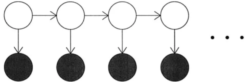
An important facet of the general BN framework is that there is no implicit temporal-ity - the network simply represents relationships between different random variables. However, we know that our POMNet model uses the same kind of temporal evolution found in HMMs, so we want to find a way to represent it. We note that an HMM can be represented as a particular type of BN, which has a simple two-node structure that repeats once for each time step of the HMM (Figure 2-1), in which, in each time slice, a hidden node represents the state of the underlying Markov chain, and an evidence node represents the corresponding observation. This type of BN, with a repeating structure over time steps, is in fact often called a Dynamic Bayesian Network (DBN) (see for instance [5], [12], or [16]).

Figure 2-1: A hidden Markov model expressed as a Bayesian network. Shaded circles represent evidence nodes.

(23)

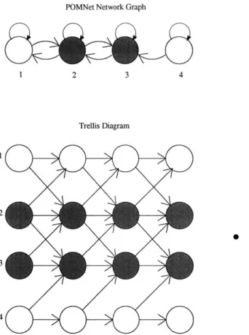
Since the POMNet can be represented as an HMM, we know that it can also be represented as a DBN. However, we can choose a much more informative and use-ful representation than the two-node repetition we used for HMMs. Considering the POMNet over a finite interval of time, we can create a DBN with one node per state variable per time step, and represent dependencies between nodes across time. The resulting directed acyclic graph, which we will call a trellis diagram, fully represents the structure of the POMNet (Figure 2-2). Note that we don't have any edges be-tween nodes within a given time step, since as we said, si[k + 1] is independent of all other state variables at time k + 1 given s[k]. Also, the directed edges always feed for-ward by exactly one time step, since we are dealing with a first order Markov process. Our partial observations constitute instantiated (evidence) nodes in the network, and consist of the same nodes at every time step of the repeating structure, since we defined partial observation over a fixed subset of nodes in the POMNet. Therefore all the structural information in this infinite trellis is contained in a snapshot of the nodes at any time, and the feed-forward edges from any time k to k + 1.

This representation of the POMNet is especially useful, as it allows us to apply some results from BNs to understand and improve the efficiency of inference tasks. Furthermore, it appears that these results can be translated to a form that is easily identified in the original POMNet or IM network graph. These tools for inference are the topic of the next chapter.

(24)

POMNet Network Graph 1 2 3 4 Trellis Diagram 2 3 4

Figure 2-2: A POMNet graph and corresponding trellis diagram. Shaded circles represent evidence nodes.

2.5 A Generalized Influence Model

We saw how a POMNet can be formulated as a Bayesian network. We now present a novel and potentially useful model which results from hybridizing the influence model and dynamic Bayesian networks in a different way than a POMNet. This can be thought of as a generalization of the IM, or equivalently a specially structured

DBN, since the influence model is a particular instance of DBN. The basic idea is

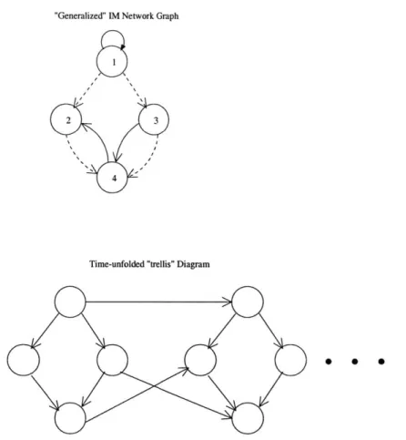
to allow for nodes within each time-slice of the model evolution to influence one an-other, resulting in same-time directed edges in the trellis diagram for the model (see Figure 2-3 for an example). In this sense, it is close to a DBN, which allows this type of same-time dependence. However, we choose to maintain the quasi-linear update

(25)

structure of the IM, and describe the same-time influence by a new influence matrix, called F, in addition to our standard network influence matrix D. The strictly lower triangular matrix F describes edge weights on a DAG (for a Bayesian network) over the nodes at a given time step, and a set of mi x mj matrices {Bij}, analogous to the

{Aij}, describes the effects of these same-time influences (now E,(dij +

fij)

1 and {Bjj} is also row-stochastic).

"Generalized" IM Network Graph

2 3

4

Time-unfolded "trellis" Diagram

Figure 2-3: A "generalized" IM graph and trellis (DBN) structure. Solid lines repre-sent influence in the usual sense, whereas dashed lines reprerepre-sent same-time influence. The order for updating nodes at each time step would be {1}, {2, 3}, {4}.

The model update can proceed in a similar fashion to the IM, with the following difference: the standard process will only update those nodes which are root nodes of the DAG, that is, those nodes whose values at time k + 1 are only influenced by the

(26)

state of the model at time k. We then add a step in which the remaining nodes at time k

+

1 are updated from the root nodes at that time (i.e. the root nodes update their children, and the updated nodes update their children, and so on). In other words, the update proceeds as follows:

1. Update the distributions for nodes dependent only on the previous time step

(without same-time influence) as in the standard IM: for such a node i,

I3

Pi[k + 1] = dij s' kAg,(.5.1)

just as in Equation 2.1.3 of the IM. We then find the realizations of those dis-tributions, obtaining si [k + 1] for this set i.

2. Update the distributions for nodes dependent only on the previous time step as well as the already-updated nodes: for such a node i,

pi[k + 1] = dis [k]AiZ + fij s [k + 1]Bji. (2.5.2)

Note that in the second sum,

fij

will be 0 for nodes j at which s [k + 1] has not yet been obtained. We find the realization of the calculated distributions, obtaining s [k + 1] for this set i.

3. Repeat Step 2 until si[k + 1] is obtained for all i, i.e. until all nodes at time

k + 1 are updated.

In order to further explore the properties of this model, we look at the conditional expectation of the system state, given the state at the previous time step. We will restrict ourselves to the homogeneous case for simplicity (analogous to the homoge-neous influence model), where the number of possible states at each node is fixed at

(27)

m, {A 3} = A and {B 3} = B.

Since a state vector is a realization of the corresponding probability vector, we still have that

E(s'[k + 1]1 s[k]) = p'[k + 1].

To further follow the IM development, we would like to represent our update equation

2.5.2 in matrix form, as in Equation 2.1.4 of the IM.

Toward this goal, we introduce some terminology to deal with the additional com-plexity of the generalized IM. Let the set of nodes n in the model be partitioned so that n=

{=ii, n2,-

, _{rq}, where ni is the first tier of nodes (root nodes of the DAG),}

n2 is the second tier which depends only upon nodes in ni and in the previous time step, etc., and q is the number of tiers. We assume from now on that the vectors and matrices describing the model as a whole are specified in this tiered ordering. Let

Nj =

IJ>=

ni for

j

= 1, - ,q, that is, N is the cumulative set of nodes up to and

including tier

j

(so that Nq= n). Let sn [k] denote the state of nodes in tier i at time

k, and sN, [k] denote the state of nodes in tiers 1 to

j

_{at time k.}

Just as H = D' 0 A (Equation 2.1.5) in the IM, we now define

G = F' o B, (2.5.3)

where F and B are as given before.

We then define the following notation for picking subsets of the matrix H:

Hi =D',

o

A,

(28)

of D corresponding to the nodes in nj. Similarly, let

GN_1 =F'NJ 1 B

where FNj-1 consists of the size Inr

I

x jNj_1 I matrix obtained from picking the rows

of F corresponding to the nodes in nr, and the columns of F corresponding to the nodes in N_1 . Finally, let

G = F' o B,

where Fn, consists of the size jnr

I

x

InjI

matrix obtained from picking the rows and columns of F corresponding to the nodes in nr. Note that

Gni

GNj_1-This notation is necessary because each time we perform Step 2 of the update (Equa-tion 2.5.2), we need to map the state vector for the previous time step s[k] and the state vector for previously computed tiers SN_1 [k + 1] on to the probability vector for tier j in a different way.

Using this terminology, and assembling Equation 2.5.2 for all sites i E nj gives

p'j [k + 1] = E(s' j [k + 1] 1s'[k, s' _1[k 1])

= s'[k]Hnj + S'Nj _1[k + 1]GN_ ₁ (2.5.4)

forjz=1,- , q.

Iterating the expectations over s[k] and sN_1 [k + 1] , we get

(29)

Moving the second term on the right hand side over to the left, we have

E(s' [k + 1]) - E(s'N _[k + 1])GN, 1 E(s'[k])Ha₃, (2.5.6)

for

j

1,.- , q. Now, combining Equation 2.5.6 for all

j

using the definitions for the subsets of G and H discussed earlier, and using a block vector/matrix notation for grouping tiers together, the left hand side becomes

I -Gn, -Gni.. -Gni

0 I -Gn2 -Gn2

E([s' 1[k+1]s'2[k+F1] . . .s'[k+1]]) 0 0 I ... -G. = E(s'[k+1])[I-G].

0 0 0 ... I

(2.5.7)

Finally, we obtain the recursive update for the expectation:

E(s'[k + 1])

[I

- G] = E(s'[k])H. (2.5.8)

Compared to the standard IM, which results in E(s'[k + 1]) = E(s'[k])H (see Equation 2.1.9), we now have E(s'[k + 1])J = E(s'[k])H, where J = [I - G], for the

evolution of the expected state vector. Using this, one is able to discuss the limiting steady state probabilities for large k. Just as the steady state distribution for the original IM depends on the eigenvalues and eigenvectors of H (see the discussion in [1] and [2]), our steady state distribution should depend on the generalized eigenvalues and eigenvectors of the matrix pair (J, H).

Note that the strictly upper triangular nature of G allows for a simple expression for the inverse of J:

j-1 = I+ G+ G2 +... + Gq-1.

This is easily verified by multiplying this expression by I - G, and noting that Gq

(30)

due to the properties of Kronecker products (see [19] for instance):

G' = (F')' 0 B.

Thus, by bringing J to the right hand side of Equation 2.5.8, the expected value recursion can be propagated forward using a matrix whose form is explicit.

This generalized influence model, motivated by DBN structure, may be able to better capture the system dynamics for particular applications, while maintaining much of the tractability and appeal of the IM.

(31)

Chapter 3 Efficient Inference: Relevance and

Partitioning

3.1 The Inference Task

Statistical inference can be described as making an estimation, making a decision, or computing relevant distributions, based on a set of observed random variables. In the context of the influence model and other graphical models, inference tasks might include: (1) calculation of the marginal distribution over a few variables of inter-est, (2) estimation of the current or future state of the system, or (3) learning the structure or parameters of the model (although learning is considered a separate task from inference in some contexts). All of these tasks require some data, and may have varying assumptions as to how much of the model we take for granted and how much we must discover. When we talk about inference in the context of graphical models, we are almost always referring to the first task, namely calculating posterior marginal distributions conditional on some data, as this will allow us to do state estimation and other things as well.

At first glance, we may think to approach such a task by considering the joint distribution of all the system variables, and marginalizing out all the random vari-ables that are not of interest. Doing this by brute force, however, is intractable for

(32)

practically any problem worth modelling with a graphical model. The key, then, is to take advantage of the special structure of the joint distribution that the graphical model captures in order to make inference tractable. The rest of this chapter will be about methods that attempt to do exactly that.

We must realize, however, that even after optimizing our algorithms with respect to a given model structure, inference may still be very complex. Computational time is often exponential in the number of nodes in our graph. In fact, it has been shown that in the most general case of a graph with arbitrary structure, both exact and approximate inference will always be NP-hard [6]. Keeping this in mind, we still try to find methods to improve efficiency for specific problems.

3.2 _{Probabilistic Independence and Separation}

3.2.1 d-Separation

In Chapter 2, we noted that the strength of Bayesian networks lies in their ability to capture conditional independence between random variables. Directional-separation, or d-separation (named so because it functions on a directed graph), is the mechanism for identifying these independencies; namely, a set of nodes A is d-separated from a set B by S if and only if the random variables associated with A are independent of those associated with B, conditional on those associated with S. Informally, this occurs in BNs because an evidence node blocks propagation of information from its ancestors to its descendants, but also makes all its ancestors interdependent.

There are several equivalent ways to define d-separation. We will first define it using the graph-theoretic terminology outlined in Chapter 2; this is the formal def-inition preferred in sources from the statistical community, such as [7] and [17]. To

(33)

"cmarrying") all pairs of parents of each node, and then dropping the directionality

of arcs. That is, if G = (V, E) is a DAG, and if u and w are parents of v, create an undirected arc between u and w. Do this for cvery pair of parents of c and for all

v E V, and then convert all directed arcs into undirected arcs connecting the same

nodes. The resulting graph is called the moral graph relative to G, and is denoted by

Gm. If a set A contains all parents and neighbors of node a, for all a E A, then A is

called an ancestral set. We will denote the smallest ancestral set containing set A by

An(A). A set C is said to separate A from B if all trails from a E A to 3 E B intersect

C. Then, the definition is as follows: given that A, B and S are disjoint subsets of a

directed acyclic graph D, S d-separates A from B if and only if S separates A from

B in (DAn(AUBUS))m, the moral graph of the smallest ancestral set containing AUBUS.

The second definition is more algorithmic in nature, and tends to be favored by the artificial intelligence community; see for instance [22]. Recall that a trail is a sequence that forms a path in the undirected version of a graph. A node a is called

a head-to-head node with respect to a trail if the connections from both the previous

and subsequent nodes in the trail are directed towards a. A trail 7r from a to b in a

DAG D is said to be blocked by a set of nodes S if it contains a vertex -y E r such that either:

1. is not a head-to-head node with respect to 7r, and - E S, or

2. - is a head-to-head node with respect to 7r, and -y and all its descendants are not in S.

A trail that is not blocked is said to be active. With this definition, A and B

are d-separated by S if all trails from A to B are blocked by S (i.e. there are no active trails). This definition lends itself to a convenient and fairly elegant method for determining d-separation called the "Bayes-ball" algorithm [27]. This algorithm determines d-separation with an imaginary bouncing ball that originates at one node and tries to visit other nodes in the graph, and at each node either "passes through,"

(34)

1. an unobserved node passes the ball through, but also bounces back balls from

children, and

2. an observed node bounces back balls from parents, but blocks balls from chil-dren.

As the ball travels, it marks visited nodes, and at the end of the algorithm (see

[27] for details), the nodes that remain unmarked are those that are d-separated from

the starting nodes given the observations. The advantage of this method is that it is simple to implement, and intuitive to follow.

As the description of the Bayes-ball algorithm makes clear, our interest in d-separation is that it will tell us which nodes are independent from others given a particular set of observations, or evidence nodes. Easily identifying independence in the graph is central to efficient inference, as we will see next.

3.3 Relevance Reasoning

3.3.1 Relevance in Bayesian networks

"Relevance reasoning" is the process of eliminating nodes in the Bayesian network that are unnecessary for the computation at hand (see [9] and [18]). The idea is to identify a set of target nodes for the inference task, and then to systematically elim-inate all nodes that will not affect the computation on those target nodes, given a set of evidence nodes, before performing inference on the graph. Since complexity is generally exponential in the number of nodes, this will greatly reduce the complexity of our computations in general - performing any inference, whether exact or approx-imate, on a graph with fewer nodes will be more efficient.

The process of eliminating nodes can be divided into three steps: (1) eliminating "computationally unrelated" nodes, (2) eliminating "barren" nodes, and (3)

(35)

eliminat-ing "nuisance" nodes. The first, and most important, step is based on the d-separation criterion. Nodes that are d-separated from all of our target nodes given the evidence are probabilistically independent of all random variables of interest, and are thus computationally unrelated to them. Once we have identified these nodes by using an algorithm such as Bayes-ball, we can remove them from our graph, reducing the number of nodes our algorithms must operate upon without changing the result.

A barren node is one such that is it neither an evidence node nor a target node,

and either has no descendants, or all its descendants are also barren. Barren nodes may depend upon the evidence, but they do not affect the computation of probabil-ities at the target nodes, and are therefore computationally irrelevant. Algorithms that identify independence can be extended, in a simple fashion, to also identify and eliminate barren nodes [18].

In order to describe the third step, once again, we need to define some additional terms. A minimal active trail between an evidence node e and a node n, given a set of nodes E, is called an evidential trail from e to n given E. A nuisance node, given evidence nodes E and target nodes T, is a node that is computationally related to

T given E (i.e. is not d-separated), but is not part of any evidential trail from any

node in E to any node in T. Elimination of nuisance nodes doesn't yield as much of a computational benefit as the first two steps, and we will not discuss them further here. It should be noted however that nuisance nodes are not removed directly - they must be marginalized into their children; see [18] for details.

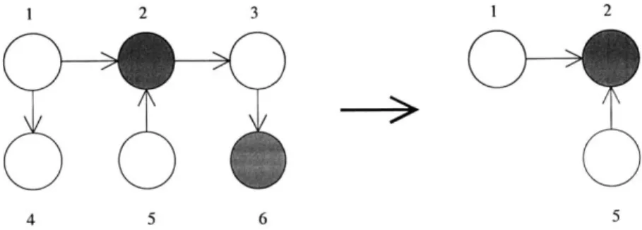
For an example of node elimination using relevance, consider the graph in Fig-ure 3-1. Let our target be node 1. We first eliminate nodes 3 and 6, as they are d-separated from node 1 by the evidence at node 2. We then eliminate node 4, as it is barren, leaving us with a significantly reduced graph on which to perform inference for our target.

(36)

1 2 3 1 2

4 5 6 5

Figure 3-1: An example of a BN graph, and the nodes relevant to target node 1. Shaded circles represent evidence nodes.

3.3.2 Relevance in the POMNet

Given that the POMNet translates readily to a Bayesian network (as a DBN), and that relevance in BNs is easily identified, it is not unreasonable to think that we might identify relevant nodes for a particular computation in the POMNet itself, without resorting to a trellis diagram. From a slightly different perspective, the notion of a

independent set in the influence model is introduced in [29]. A (-independent set A is

defined as follows (with respect to the network influence graph of the POMNet/IM):

1. All incoming links to A originate from evidence sites.

2. All outgoing links from the non-evidence sites of A terminate in non-influencing sites, where a non-influencing site is defined as one from which there exists no path to an evidence site.

The goal of identifying (-independence is equivalent to that of eliminating irrele-vant nodes - to reduce inference to the simplest possible calculation for a particular set of sites. We claim that applying relevance reasoning in the POMNet trellis is in fact equivalent to proceeding by (-independence. In particular, by selecting a set of sites in a POMNet and running the relevance algorithms on the corresponding BN with the time-extended version of the selected sites as target nodes, the resulting set of nodes

will be the smallest (-independent set containing the selected sites, and thus the

con-cepts of relevance and (-independence are equivalent in this sense. This can be seen as follows: if all incoming links to A are from evidence sites, then all incoming arcs to the

(37)

set of nodes corresponding to A are from evidence nodes. These nodes are not head-to-head nodes with respect to any paths connecting A to the nodes outside of A, and thus they block those paths (by our second definition of d-separation above). Addi-tionally, all outgoing links from A terminate in non-influencing sites. Non-influencing sites correspond to barren nodes in the trellis diagram, and thus these outgoing links can be removed. Finally, evidence sites in A with only outgoing links leaving A can never be head-to-head nodes along any path leading out of A, and therefore block the remaining paths. So, we see that the conditions for (-independence induce a set of nodes that can be obtained from relevance reasoning. Thus a possible use for the (-independence conditions is to directly and intuitively identify sets of sites in a POMNet that would be produced by relevance reasoning in the corresponding trellis, without resorting to an analysis of d-separation and barrenness in the underlying BN.

This idea of obtaining minimally-relevant subsets of the graph (in both BNs and POMNets) lends itself to simplifying inference in a complex graph by identifying sub-graphs that can be dealt with separately. The process of breaking the graph up into such subgraphs is referred to as relevance-based decomposition

([18]),

or partitioning

([29]). Note that in the general case of decomposition, these subgraphs will be

par-tially overlapping, especially sharing evidence nodes. Algorithms for decomposing the graph in this way can be as simple as arbitrarily choosing small subsets of target nodes, and eliminating irrelevant nodes for each such subset; however, the particular choices of subsets will significantly affect the efficiency of the algorithm. Although even crude choices of target subsets will improve overall performance ([18]), ways of optimizing this process remain to be studied in greater detail.

(38)

3.4 Algorithms for Exact Inference

3.4.1 Message Passing and the Generalized Forward-Backward

Algorithm

The generalized forward-backward algorithm is an exact inference message passing algorithm for singly connected connected Bayesian networks [11]. As the message passing algorithm (due to Pearl

[23])

works in polynomial time, it is the method of choice for inference in singly connected networks.

Message passing (also called probability propagation, or belief propagation, al-though the latter often refers to loopy belief propagation, discussed later) is a mecha-nism by which information local to each node is propagated to all other nodes in the graph so that marginalization can be performed. The forward-backward algorithm arranges this message passing in a highly regular way by breaking the process into two parts: a forward pass, in which information is propagated towards an arbitrarily cho-sen "root" node (also known as "collecting evidence"), and a backward pass in which information is propagated away from the root ("distributing evidence"). There are two types of computation performed in this process: multiplication of local marginal distributions at each node, and summation over local joint distributions (this is why it is also sometimes called the "sum-product algorithm") (see [11]), so that the outgoing message from each node consists of the product of all incoming messages, summed over the local distribution.

We will call a message from a child to a parent a A message, and the message from a parent to a child a 7r message. A node can calculate its i message to its children once it receives 7r messages from all its parents, and can calculate its A message once it receives A messages from its children. The local posterior distribution at a node can be found once it has calculated both its A and 7r messages, by multiplying the two.

(39)

For a simple example.

let

us look at message passing on a directed chami. i <-

j

k (that is, a, node

j

with unique child i and unique parent k). We pick node k as

the root, and the generalized forward-backward message passing order will then be as follows: Ai-,, Aj-k, 7k-j, 7j. In this example (from [20]), the A message from

j

to k is

and the 7 message from

j

to i is

k

As mentioned in [20], and as we might expect, in this case the algorithm is equivalent to the forward-backward algorithm for HMMs, where r is the equivalent of the for-ward variable a and A is the equivalent of the backfor-ward variable 3, and where A and 7r can be computed independently of each other (this is not generally the case in a tree).

3.4.2 The Junction Tree Algorithm

The standard algorithm for exact inference on a multiply connected Bayesian network is the so-called

junction

tree or

join

tree algorithm (see for example [21]). This concept

is sometimes also referred to as clustering when a tree is created from clusters, or groups, of variables in a complex problem. The junction tree algorithm proceeds

by first creating a "junction tree" out of the BN graph, which is a representation

that allows a potentially complex graph to be expressed in an easily manipulated

(and singly connected) tree form. The process of building a junction tree can be summarized in the following steps:

1. Moralize the graph. As mentioned previously in the context of d-separation, moralization involves "marrying" common parents, and converting the graph to its undirected form.

(40)

if it (loesil't

li'iy&

r111v cvcles of lel-ti -ive(i thwn 3. Triiaiiguilat e G,

by adding chords as necessary.

3. Find the maximal cliques. Group the nodes in each clique together - each clique will make up a node of the junction tree.

4. Connect the cliques in a tree.

Once the tree is created, message passing algorithms that work on singly con-nected graphs are will efficiently solve the inference task.

However, this method is not without its flaws. Following the above steps to

cre-ate a junction tree doesn't result in a unique solution, and some junction trees will result in more efficient solutions than others - this arises from the fact that there are often many different triangulations of a given graph. In fact, finding the opti-mal triangulation (i.e. leading to the most efficient inference possible) is itself an NP-complete problem [13]. For this reason, the junction tree algorithm is sometimes used with approximately optimal triangulation methods. Still, it has been shown that any exact inference method based on local reasoning is either less efficient than the junction tree, or has an optimality problem equivalent to that of triangulation [13].

3.4.3 Exact Inference in the POMNet

We now turn to inference in the POMNet model. Since we know that a POMNet trellis is in fact a DBN, and that it will be multiply connected in all but the most degenerate cases, we might think to immediately apply the junction tree algorithm (preferably after eliminating extraneous nodes through relevance reasoning). For de-tailed treatment of junction tree inference in DBNs, see [16] or [20].

An alternate way to approach this problem, discussed in [29], is to develop a method by analogy with the HMM forward-backward algorithm. This entails defining

(41)

le1n(rsivelv computed forward and backward variables. which in fact can be computed

locally to any (-independent subset of the POMNet ((-independence was defined in section 3.3.2). We assume that we have data in the form of observations (at the ob-servable sites) from time 1 to T. The local forward variable a' [k] of a (-independent set A is defined as the probability that the hidden sites of A (the state of which will be denoted by A[k]) are in a particular state i at time k, given the portion of the observations up to some time k (denoted Q1'k):

c4[k]

e P(A[k = zQ1k) Just as in the HMM, the backward variable 3f'[k is defined such that the product of forward and backward variables will result in the posterior marginal distribution that we de-sire, that is, aA[k]O[k] = P(A[k] =7 101,T). Thus, we perform the inference task by

computing the forward and backward variables for any intermediate time k (see [29]).

The standard forward-backward algorithm for HMMs can itself be applied to a POMNet as well, since we can simply formulate our POMNet as an HMM, as de-scribed earlier. We do not compute variables local to subsets of the graph in this case, but we can eliminate computationally irrelevant sites before converting to an HMM, and so can still perform relevance-decomposed inference. Further variations on the forward-backward algorithm are also used in the context of DBNs. Just as the forward-backward algorithm exploits the Markov structure of HMMs by conditioning on the present state to make the past and future hidden states independent, the

fron-tier algorithm exploits the Markov structure of DBN models by conditioning on all

the nodes at a particular time step to separate the past from the future, updating the joint distribution with a forward and backward pass that maintain such a separating set at every step [20]. Similarly, the interface algorithm attempts to improve upon this strategy by identifying the minimal set of nodes needed to d-separate the past and fu-ture based on the graph strucfu-ture, thereby proceeding in a more efficient manner [201.

(42)

3.5 Algorithms for Approximate Inference

In many problems of practical interest that map to multiply connected networks, even the most efficient exact inference algorithms are intractable [11]. Although the approximate inference task has also been shown to be NP-hard in the general case

[18],

approximations can potentially make inference tractable, with each approxima-tion algorithm best suited to a particular class of problems. Approximate inference algorithms can be divided into two categories: (1) stochastic methods, which include such Monte Carlo methods as Gibbs sampling, importance sampling, and a sequential method called particle filtering, and (2) deterministic approximation methods, two of which are described below.

3.5.1 Variational Methods

Variational methods are a commonly used approximation technique in a wide variety of settings, from quantum mechanics to statistics [14]. [14] also provides a compre-hensive tutorial on their use in the context of graphical models. The basic idea can be summarized as follows: in this context, we use variational methods to approach the problem of approximating the posterior probability distribution P over the hid-den nodes by defining a parameterized distribution

Q,

and varying its parameters to minimize the distance between P and

Q.

Since the complexity of inference in the approximation given by

Q

is determined by its conditional independence relations, we can choose

Q

to have a tractable structure, such as a Bayesian network with fewer dependencies than P [12]. We then minimize the distance between P and

Q

with respect to a metric such as the Kullback-Leibler divergence.

3.5.2 "Loopy" Belief Propagation

So-called "loopy" belief propagation is simply the message passing/probability prop-agation algorithm described previously, applied to multiply connected graphs (i.e.

(43)

containing loops in the underlying undirected graph). While this method will not in general converge to the correct marginal distributions in a short time, as it does in the singly connected case (e.g. two passes for the generalized forward-backward algorithm), it is in many cases guaranteed to converge to a set of locally consistent messages. The accuracy and optimality of this algorithm have been studied to some degree, including potential ways to correct the posterior marginals after convergence

(see [30]). Loopy belief propagation has been found to produce good results in a variety of fields with large scale applications for graphical models, including decoding turbo codes, image processing, and medical diagnosis.

(44)

Aspects of inference for the Influence Model and related graphical models

Aspects of Inference for the Influence Model and

Related Graphical Models

by

Arvind K. Jammalamadaka

B.S., University of California at Santa Barbara (2001)

Submitted to the Department of Electrical Engineering and Computer

Science

in Partial Fulfillment of the Requirements for the degree of

Master of Science in Electrical Engineering and Computer Science

at the

Massachusetts Institute of Technology

June 2004

@

Massachusetts Institute of Technology 2004. All rights reserved.

A uthor ...

...

Department of Electrical Engineering and Computer Science

May 21, 2004

Certified by ...

George C. Verghese

Professor of Electrical Engineering

Thesis Supervisor

Accepted by ..

Arthur C. Smith

Chairman, Department Committee on Graduate Students

Aspects of Inference for the Influence Model and Related

Graphical Models

by

Arvind K. Jammalamadaka

Abstract

Dedicated to:

Acknowledgments

Contents

List of Figures

Chapter 1

Introduction

[4].

1.1

Overview

Chapter 2

The Influence Model and Related

Graphical Models

2.1

The Influence Model

2.1.1

Definition

j,

1]Is[k])

2.1.2

An Alternate Formulation

[k].

j

2.1.3

Expectation Recursion

1

I

2.1.4

Homogeneous Influence Model

2.1.5

Matrix-Matrix Form

2.2

Partially Observed Markov Networks

2.2.1

Markov Networks

2.2.2

Partial Observation

2.3

Relation to Hidden Markov Models

2.3.1

Hidden Markov Models

2.3.2

Relation to the POMNet

2.4

Relation to Bayesian Networks

2.4.1

Bayesian Networks and Graph Theory

4,

4

4,

_{Probabilistic Independence and Separation}