Publisher’s version / Version de l'éditeur:
Proceedings of the 6th International Symposium on Radiative Transfer, 2010
READ THESE TERMS AND CONDITIONS CAREFULLY BEFORE USING THIS WEBSITE.
https://nrc-publications.canada.ca/eng/copyright
Vous avez des questions? Nous pouvons vous aider. Pour communiquer directement avec un auteur, consultez la première page de la revue dans laquelle son article a été publié afin de trouver ses coordonnées. Si vous n’arrivez pas à les repérer, communiquez avec nous à [email protected].
Questions? Contact the NRC Publications Archive team at
[email protected]. If you wish to email the authors directly, please see the first page of the publication for their contact information.
NRC Publications Archive
Archives des publications du CNRC
This publication could be one of several versions: author’s original, accepted manuscript or the publisher’s version. / La version de cette publication peut être l’une des suivantes : la version prépublication de l’auteur, la version acceptée du manuscrit ou la version de l’éditeur.
Access and use of this website and the material on it are subject to the Terms and Conditions set forth at
Soot particle sizing by inverse analysis of multiangle elastic light scattering
Burr, D. W.; Daun, K. J.; Link, O.; Thomson, K. A.; Smallwood, G. J.
https://publications-cnrc.canada.ca/fra/droits
L’accès à ce site Web et l’utilisation de son contenu sont assujettis aux conditions présentées dans le site
LISEZ CES CONDITIONS ATTENTIVEMENT AVANT D’UTILISER CE SITE WEB.
NRC Publications Record / Notice d'Archives des publications de CNRC:
https://nrc-publications.canada.ca/eng/view/object/?id=f0f5e4c1-3dfc-4127-9961-89d9162256b2 https://publications-cnrc.canada.ca/fra/voir/objet/?id=f0f5e4c1-3dfc-4127-9961-89d9162256b2
SOOT PARTICLE SIZING BY INVERSE ANALYSIS OF MULTIANGLE ELASTIC LIGHT SCATTERING
D. W. Burr1, K. J. Daun1, O. Link2, K. A. Thomson2, and G. J. Smallwood2
1
Department of Mechanical and Mechatronics Engineering, University of Waterloo, Waterloo, ON N2L 3G1, Canada
2
Institute for Chemical Process and Environment Technology, National Research Council Canada, Ottawa, ON K1A 0R6, Canada
ABSTRACT. Recovering the size distribution of aerosolized soot aggregates from multiangle elastic light scattering data requires solving an inverse problem. This paper presents a methodology that uses maximum à posteriori (MAP) inference to stabilize the inversion by introducing prior information about the size distribution of the soot aggregates.
INTRODUCTION
In most combustion processes unburned pyrolized fuel forms nanospheres called primary particles, which in turn agglomerate into polydisperse fractal soot aggregates. The impact of these aggregates on human health [1] and the environment [2] is a function of their transport properties and absorption and scattering cross-sections. Given the dependence of these attributes on aggregate morphology, especially the number of primary particles per aggregate, there is a need for instruments that quickly and accurately characterize the size distribution of aerosolized soot aggregates.
One way to do this is by extracting aggregates directly from the aerosol by thermophoresis and then imaging them using transmission electron microscopy (TEM). This method is time consuming, however, and results may be biased since certain particle sizes may be preferentially attracted to the TEM slide, among other factors [3]. An alternative is to shine collimated light through the aerosol and then infer the aggregate size distribution from the angular distribution of scattered light [4]. This method potentially gives more spatial and temporal refinement than physical probing, and a properly-calibrated instrument can provide near-instantaneous results.
Most often, particle sizing through multiangle light scattering is done by assuming the aggregates obey a prescribed (usually lognormal) distribution type and then determining the distribution parameters that best explain the data, either by analyzing features of the curve formed by plotting angular scattering intensity versus the scattering wave vector [4-7], or through least-squares fitting to experimental data [8, 9].
Unfortunately, these procedures often produce ambiguous solutions due to the fact that the soot aggregate size distribution is related to angular scattering measurements by an integral equation,
(1) 1 ( ) ( p) ( , p) d g C P N K N N ∞ =
∫
θ θ pwhere g(θ) is the measured scattering data, Np is the number of primary particles per aggregate,
derived from light scattering theory. The coefficient C scales the scattered light intensity to the detector signal, and is often a function of P(Np) as described below. Recovering P(Np) from Eq. (1)
is mathematically ill-posed because the solution is not unique or stable; instead, an infinite number of aggregate size distributions satisfy Eq. (1) within experimental accuracy.
Consequently, this ill-posed problem must be solved by augmenting the deficient information provided by multiangle light scattering with assumed attributes of P(Np), called priors. Since priors
are usually only a “guess” and may not describe P(Np) exactly, they must be assigned appropriate
influence on the recovered solution. For example, enforcing a lognormal distribution for P(Np) is
not ideal since the true distribution may not be exactly lognormal; due to the ill-posed nature of Eq. (1), however, a lognormal P(Np) may indeed exist that explains g(θ), leading one to the potentially
erroneous conclusion that P(Np) is lognormal.
A few studies have avoided constraining P(Np) to a presumed distribution type by transforming Eq.
(1) into an ill-conditioned matrix equation, Ax = g, where x is a discrete form of P(Np), and then
solving x through regularization. Twomey [10] was the first to do this by linear and then iterative regularization; the latter technique was later improved by Markowski [11]. More recently di Stasio et al. [12] used Tikhonov regularization [13] to recover soot primary particle size distributions from small angle X-ray scattering data.
In this paper we use a formalized Bayesian methodology called maximum á posteriori (MAP) inference [14] to recover a soot aggregate size distribution from multiangle elastic light scattering data. Unlike other methods (e.g. [4-9]) MAP inference explicitly assigns the influence of each prior on the recovered solution. We start by deriving Eq. (1), follow with a brief review of MAP inference, and then validate the inverse methodology by recovering a distribution from an artificial data set. Finally, the method is applied to experimental data and the recovered distribution is compared to TEM data collected under identical operating conditions.
MULTIANGLE LIGHT SCATTERING FROM A SOOT-LADEN AEROSOL
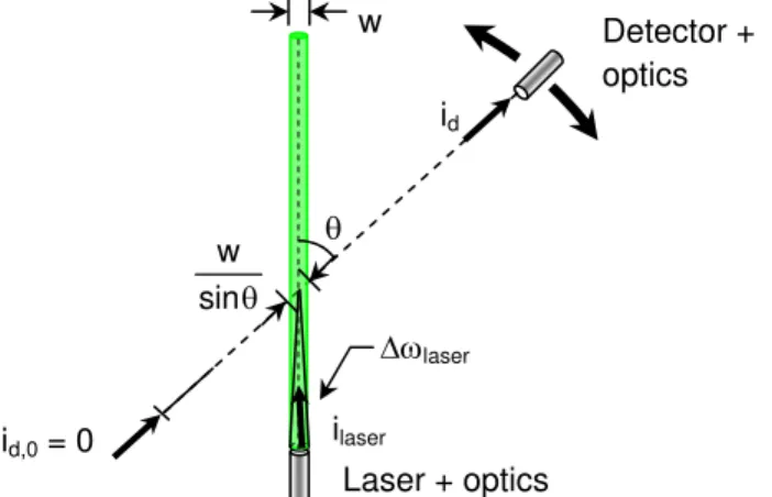
Equation (1) is derived from the radiative transfer equation for the experimental geometry shown in Fig 1. Signal trapping between the measurement volume and the detector is assumed to be negligible, which is reasonable for optically-thin flames [8]. The background “bleed-through” intensity due to soot incandescence is also negligible at the detection wavelengths; accordingly, the detector signal is due only to out-scattering of laser light into the detector direction within the measurement volume formed by the laser beam and the detector viewing cone,
( )
( )
4 0 ( ) ( , ) ( , ) d sin( ) 4 4 sin( ) Δ Φ= = exp s
∫
Φ ≈ laser laser sexp d d i d i i C w w i g C i i π σ ω θ θ ω κ ω ω ω ω σ θ π π θ (2)
where Φ(ωd, ωi) is the spectral scattering phase function, σs is the spectral extinction coefficient,
ilaser is the laser intensity (assumed here to be vertically-polarized), θ is the angle between ωd and
the laser propagation direction, w is the beam width, and Δωlaser is a small but finite solid angle
subtended by the laser beam. The constant Cexp relates the incident intensity to the detector signal,
and accounts for the collection optics and photoelectric conversion efficiencies. Although Eq. (2) assumes a spatially-uniform beam profile, the error caused by using a beam with a Gaussian intensity distribution is quite small.
We now relate Φ(θ) and σs to the soot particle morphology through Rayleigh-Debye-Gans
Polydisperse Fractal Aggregate (RDG-PFA) theory [15]. For vertically-polarized laser light, the phase function and scattering coefficient are given by
( ) 4 agg vv agg s C C Φθ = π (3) and
Figure 1. Schematic of multiangle light-scattering experiment
agg s =NaggCs
σ (4)
where Nagg is the aggregate number density and Csagg and vvagg
( )
C are the average scattering and vertical polarization cross-sections of the soot aggregates. The product σs⋅Φ(θ) then becomes
( )
(
)
1 4 agg 4 agg ,( )
d s πNaggCvv θ πNagg Cvv Np ∞ =∫
P Np Np σ ⋅Φ θ = θ(
(5) The vertical polarization cross-section of a soot aggregate is)
2( )
( )
, agg p vv p p vv g p C N θ =N C f q⎡⎣ θ ⋅R N ⎤⎦ p C(
)
(6) where q(θ) ≡ 2η sin(θ/2) is the modulus of the scattering vector, Rg is the radius of gyration, vv ≡xp6F(m)/η2 is the polarization cross-section of a primary particle, η ≡ 2π/λ is the wave number, xp ≡
πdp/λ is the size parameter, F(m) = |(m2−1)/(m2+1)|2 is the complex scattering function, m is the
complex index of refraction, and f(⋅) is the form factor.
Collecting all the constants together shows that the detector intensity is related to the size distribution by Eq. (1), where the kernel contains terms that depend on Np and θ,
( )
( )
2 , sin p g p p N f q R N K N ⎡ ⋅ ⎤ ⎣ ⎦ = θ θ θ (7)and the remaining terms are absorbed into the coefficient,
( )
6 2
2 Δ
=C wexp laser laseri Naggx Fp
C ω
η
m
(8) The radius of gyration indicates the size of the soot aggregates. Most flame-synthesized soot
aggregates obey the fractal relationship Np = kg(2Rg/dp)Df, with kg = 2.3 and Df = 1.78 being typical
fractal prefactors and exponents [5]. This expression is rearranged to give
( )
dp(
Np kg)
1 Df( )
( )
2
g p
R N = (9)
The form factor, f [q(θ)Rg(Np)] has been derived in a number of different forms over the Guinier
and power-law regimes. The model for the form factor that we have chosen is [16]
( )
/8 2 8 8( ) 1 3 f D g g p g f qR f q R N qR D − ⎡ ⎤ ⎡ θ ⎤= +⎢ + ⎥ ⎣ ⎦ ⎢ ⎥ ⎣ ⎦ (10)which is valid over both regimes.
Detector + optics Laser + optics w θ θ w sin id Δωlaser ilaser id,0 = 0
Examination of Eqs. (1) and (8) shows that this is a linear inverse problem only if Nagg is known. In
most experiments, however, Nagg is inferred from an independently-measured soot volume fraction,
fv, by
( )
2 2 1 d v v agg p p p p p f f N d N d N P N N π π ∞ = =∫
p (11)making this problem nonlinear, since C = C(Np.) In the next section we show that this nonlinear
problem can be linearized by temporarily assuming C is known at each iteration, solving the linear inverse problem, and then updating the estimate of C. Solving for C is similar in principle to examining the normalized angular scattering distribution instead of absolute intensities [9]. Also note that C isolates many of the parameters subject to large degrees of uncertainty (including m), which can be an advantage over other solution methodologies.
MAXIMUM A POSTERIORI INFERENCE
With this framework in place Eq. (1) is transformed into a matrix equation, Ax = g, by setting an upper limit for the aggregate size, Np,max and then discretizing Np into n uniform strips over which
P(Np) is assumed to be uniform, as shown in Fig 2. Each element of A is found by numerically
integrating over a strip of width ΔNp,
(
)
, , 2 * 2 , d p j p p j p N N ij i p p N N * A C K θ N +Δ −Δ =∫
N (12) while gi = g(θi) and xj = P(Np,j).The underlying ill-posedness of Eq. (1) causes A to be ill-conditioned, so the matrix equation cannot be solved using conventional linear algebra tools. Instead, we must augment the information provided by Ax = g with prior assumptions about P(Np). MAP inference provides a
formalized and generic way to do this. The basis of this method is Bayes’ theorem
( )
( )
( )
model( )
P P P P = g x x g x g (13)where P(x|g) is the probability of x being correct given an observed dataset, g, P(g|x) is the probability of the data in g actually occurring for a given x (also called the likelihood function), P(g) is the marginal probability of the data, and Pmodel(x) is the probability that the solution is
correct based on assumed priors. The goal, then, is to find x* that maximizes P(x|g), usually through nonlinear programming. (Since P(g) only scales Eq. (13) it can be ignored.)
Relying solely on the multiangle elastic scattering data without making additional assumptions about P(Np) is equivalent to maximizing Eq. (13) with Pmodel(x) = 1. For a linear model, g = Ax,
and assuming the data in g is contaminated with Gaussian-distributed error having the same variance σ2
(which can be done by rescaling),
( )
2 2 2 1 exp 2 P σ ⎡ ⎤ ∝ ⎢− − ⎥ ⎣ ⎦ g x Ax g (14)Thus P(g|x) is maximized by minimizing Ax g− 22, but again, since A is ill-conditioned, there exists a large set of solutions that “almost” minimize 2
2
−
Ax g .
We must stabilize the solution of x* by adding priors to Eq. (14); since P(x|g) is the union of the likelihood function and Pmodel(x), the priors are simply multiplied on to Eq. (14) as they are
introduced into the problem. The Gibbs prior is appropriate for problems in which x should obey a smooth distribution,
( )
(
2)
exp Gibbs P x ∝ −β Lx( )
H( )
n nonneg j P x =∏
x( )
( )
2 (15)where L is the smoothing matrix. One choice for L is a discrete approximation of the derivative operator [13], so that Eq. (15) is minimized when all the elements of x are identical. The heuristic parameter β determines the importance of this prior relative to the likelihood function and other priors.
In this problem the elements of x should also be strictly nonnegative, which is enforced using
(16)
1
j=
where the Heaviside step function, H(xj), is zero if xj < 0 and is otherwise taken to be unity.
A final source of information is provided by the fact that the aggregation dynamics in the aerosol generates a self-preserving distribution that usually resembles a lognormal distribution [4, 17]. Instead of forcing a lognormal distribution, as is done in [4-9], we define a prior that promotes a lognormal distribution [18] 2 * 2 exp dist dist P = ⎡⎢−α − ⎤⎥ ⎣ ⎦ x x x θ (17)
where θ∗ are the parameters of the lognormal distribution that best matches the current estimate of x, found by minimizing the Kolmogorov-Smirnov goodness-of-fit statistic, and xdist(θ*) is generated
by evaluating the corresponding distribution at the center of each strip in Fig. 3. Equation (17) quantifies how much x resembles a lognormal distribution, while α determines the emphasis this prior has relative to the likelihood function and the other priors.
Combining these priors with P(g|x) and defining λ2 = 2σ2β
and γ2 = 2σ2α results in
( )
(
2 2( )
2(
2 2 * 2 2 2 1 exp H n dist j P λ γ x = ∝ − − − − − ⋅∏
x g Ax g Lx x x θ)
j)
( )
(18) Finally, due to the monotonicity of the logarithm function, maximizing Eq. (18) is equivalent tosolving the constrained least-squares minimization problem
2 *
* 2
arg min arg min 0 . . 0
( ) dist f s t ⎡ ⎤ ⎡ ⎤ ⎢ ⎥ ⎢ ⎥ = = ⎢ ⎥ −⎢ ⎥ > ⎢ ⎥ ⎢ ⎥ ⎣ ⎦ ⎣ ⎦ λ γ γ A g x x L x x I x θ (19) Figure 2. The integral equation is transformed into a matrix equation by representing P(Np) with
strips of finite thickness.
0 0.005 0.010 0 50 100 150 200 250 Np P(N p ) ΔNp 0.015 0.020 ( ) ( ) ( ) ( ) ∞ +Δ = −Δ θ ≈ θ ∫ ∑ p, j∫p p, j p p p p 1 N N 2 n p,j p,j p j 1 N N 2 P N K ,N dN P N K ,N dN
where I is the identity matrix. Equation (19) is actually a generalization of other methods used to solve this problem: augmenting the likelihood function with Eq. (15) alone is Tikhonov regularization [13]; while limγ→∞(x*) is equivalent to least-squares fitting a presumed distribution to
experimental scattering data in g.
As noted above, this problem is linear only if Nagg is known, which is not often the case. (Equation
(17) also makes this problem nonlinear.) We will show how to solve for C by performing a univariate minimization of f[x*(C)] later in the paper.
DECONVOLUTION OF ARTIFICIAL DATA
We first consider an artificial case representing a scenario in which Nagg (and thus C) is known by
some independent means, which makes Eq. (1) a Fredholm integral equation of the first-kind. As a test case we select a lognormal distribution known to reflect the soot aggregate size distribution determined through TEM analysis of soot sampled from an ethylene laminar diffusion flame at the location and under the operating conditions described in [8]. We use image processing software and the projected area method [3] to analyse hundreds of TEM images, which are combined with other images taken from a previous study carried out under identical conditions [19] to generate a histogram approximation of P(Np). The bins are aggregated to form approximate points on the
cumulative distribution function (CDF), to which we fit a lognormal CDF by least-squares minimization. The resulting distribution is
( )
(
,)
2 2 ln ln 1 exp 2 ln ln 2 p p g p g p g N N P N N ⎡ − ⎤ ⎢ ⎥ = − ⎢ σ ⎥ σ π ⎣ ⎦ (20) with Np,g = 23.14 and σg = 3.35. Artificial angular scattering data is then generated by substitutingthis distribution into Eq. (1) and numerically integrating at uniformly spaced measurement angles between 10° and 160°. This data is contaminated with artificial noise sampled from a normal distribution having a 3% standard deviation relative to each data point, typical of measurement noise observed in the experiment. The A matrix is formed by taking Np,max = 500 and splitting
domain into 55 uniformly-spaced bins. The rows of Ax = g are then rescaled to make the error covariance of each element of g approximately equal.
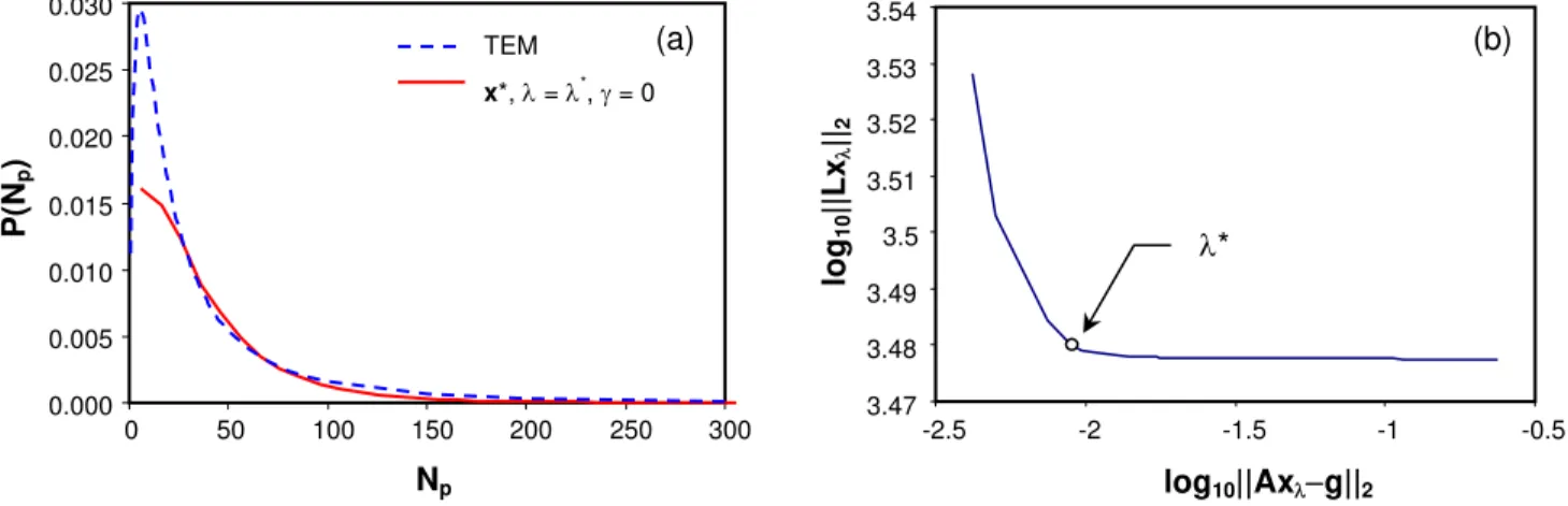
We then attempt MAP inference with Gibbs and nonnegativity priors but without assuming a distribution type, which is equivalent to first-order Tikhonov regularization with a nonnegativity constraint. While λ could be chosen heuristically, we instead use the L-curve curvature method [20] that finds the λ corresponding to the point of maximum curvature on a parametric plot of log10(||Lxλ||2) versus log10(||Axλ−g||2), where xλ is the constrained Tikhonov solution for a given λ.
This value of λ is then substituted into Eq. (19) with γ = 0 to find x*.
Figure 3 shows that the recovered distribution closely matches the assumed distribution at large Np,
but departs the assumed distribution at smaller Np. The kernel function is strongly weighted by
large aggregate sizes due to the quadratic dependence on Np found in the numerator implying that
less information is conveyed by smaller particles, a well-known limitation of multiangle elastic light scattering experiments [4]. Nevertheless, this result shows that P(Np) may be reconstructed
without assuming a distribution type, as long as C is known.
DECONVOLUTION OF EXPERIMENTAL DATA
We next apply the inverse methodology to experimental data collected at the same location and under the same experimental conditions described above. The laser source is a diode-pumped, Q-switched Nd-YLF laser with a wavelength of 527 nm and average power of 400 mW at 10 kHz. The laser beam is expanded to a 3 mm diameter and then propagates through a combination waveplate and polarizer that fine-tunes the laser energy. A second waveplate controls the final
0.030 3.54
polarization, which is vertical. A final lens focuses the laser beam to a diameter of 150 μm. The detection optics is mounted on a rotation stage centered on the soot source. The detector angle is controlled by an aperture of 10 mm diameter mounted 14 cm from the center of rotation, which in turn is followed by a bandpass filter for 527 nm, and a pair of optically-conjugate lenses that focus the probe volume onto a final detector aperture. Details of the flame and scattering optics are provided in [8] and [9], respectively.
Scattering data is collected at 5° intervals between 10° and 40°, and at 10° intervals between 40° and 160°, for a total of 19 angular measurements. Following [9], a size distribution is first recovered assuming a lognormal P(Np), by performing a least-squares minimization between the
measured and modeled data
(
)
(
)
2 , , 1 1 , , , , 2 = ⎡ ⎤ =∑
n ⎣ exp− mod ⎦ p g g j j p g g j F N σ b b θ N σ C (21)where bmod(θj, Np,g, σg, C) is found by substituting the arguments into Eq. (1) and integrating
numerically. As noted above, this is equivalent to minimizing Eq. (19) with λ = 0 and γ→∞. The solution found by nonlinear least-squares minimization is Np,g = 19.4 and σg = 1.94 but Fig. 4
shows that, due to the underlying ill-posedness of Eq. (1), this minimum is surrounded by a long, shallow valley containing solutions that explain the observed data almost as well as does the minimizer of F(Np,g,σg), including the lognormal distribution inferred from the TEM analysis. Note
that Fig. 4 only represents the set of plausible lognormal distributions that could explain the observed data; other distribution shapes are also possible.
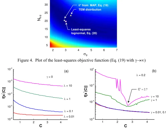
We next attempt to recover the size distribution by minimizing Eq. (19) for x and C, with γ = 0. We do this by univariate minimization of f [x*(C)], where x*(C) in turn minimizes Eq. (18) for a given
C. Unfortunately, Fig. 5 (a) shows that this function lacks a distinct local minimum for C regardless of λ. In other words, the smoothness and nonnegativity priors are insufficient to obtain a robust estimate for C*; instead, an infinite set of solutions for x and C exist that explain the observed data subject to these priors, and it is therefore necessary to add more prior information through Eq. (17). Accordingly, we repeat the process with λ = 0.2 (chosen heuristically) and various values of γ. Figure 5 (b) shows that robust estimate for C* emerges for γ > 1. The corresponding distribution for x* is shown in Fig. 6 (a), along with the best-fit least-squares distributions to the angular scattering data and the TEM histograms; the parameters contained in θ*
for the best-fit lognormal are also plotted in Fig. 4. Both show that the recovered solution is close to the distribution obtained by minimizing Eq. (21), which one would expect given that both rely on
Figure 3. (a) Distribution found using constrained Tikhonov regularization (γ = 0), and (b) corresponding L-curve for constrained Tikhonov
(a) 0.000 0.005 0.010 0.015 0.020 0.025 0 50 100 150 200 250 300 Np P(N p ) TEM 3.53 x*, λ = λ*, γ = 0 3.52 3.51 3.5 3.47 3.48 3.49 -2.5 -2 -1.5 -1 -0.5 log 10 ||Lx λ ||2 (b) log10||Axλ−g||2 λ*
Figure 4. Plot of the least-squares objective function (Eq. (19) with γ→∞)
Figure 5. (a) Smoothness and nonnegativity priors alone do not provide enough information to find C*, but (b) a robust estimate is found by promoting a lognormal distribution.
5 10 15 20 25 30 35 2 3 4 5 6 7 σg Np,g TEM distribution Least-squares lognormal, Eq. (20)
θ* from MAP, Eq. (19)
10-2 0
the optical scattering data, and a unique MAP solution is found only by promoting a lognormal distribution.
Nevertheless, Fig. 6 (b) shows that all the distributions produce angular scattering data indistinguishable from the original experimental data; this is also reflected in Fig. 4 by the flat topography in the vicinity of the three solutions. This result underscores the fact that angular scattering data by itself is insufficient to uniquely specify P(Np), and it is crucial to introduce
additional information to the problem through priors.
Although Fig. 5 shows that a robust estimate for C* and x* can be found only by promoting a lognormal distribution, unlike other implementations in which x* is forced to be lognormal, MAP inference allows x* to deviate from the presumed distribution if information provided by the angular light scattering data and other priors contradicts a lognormal distribution.
CONCLUSIONS
Inferring an aggregate size distribution from multiangle elastic light scattering data involves solving an integral equation. In this paper, we transform this equation into an ill-conditioned matrix equation and then solve it using MAP inference, which stabilizes the inversion by adding prior information about the solution characteristics. While it is possible to recover P(Np) using only
smoothness and nonnegativity priors if Nagg is known, we must add an additional prior that
promotes a specified distribution type if this parameter is unknown. Accordingly, we use MAP
λ = 0.1 λ = 0.01 1 2 3 4 10-6 10-4 10-2 10 f[x * (C )] C C (a) (b) λ = 0.2 1 2 3 4 10-6 10-5 10-4 10-3 λ = 10 λ = 1 f[x * (C )] γ = 0 γ = 0.01, 0.1 γ = 1 γ = 10 C∗ = 2.7
inference to recover a size distribution by promoting a lognormal distribution. The recovered distribution is similar to a distribution obtained by least-squares fitting to angular scattering data, and similar to one obtained from a TEM-derived histogram of aggregate sizes; substituting these distributions into the governing equation produces artificial angular light scattering data nearly indistinguishable from the experimental data.
Figure 6. (a) The recovered distribution using λ = 0.2 and γ = 1 and lognormal fits to the TEM histogram and angular scattering data all explain the experimental data (b).
This similarity highlights the importance of using additional information to mitigate the inherent ambiguity of this inverse problem. In the future we will derive more formal ways of combining information from multiple sources, such as TEM data and aerosol dynamics theory, into a MAP inference formalism for recovering soot aggregate size distributions.
ACKNOWLEDGEMENTS
This work is supported by the Natural Resources Canada PERD AFTER Program, Project C23.006, administered by Mr. Jean-Francois Gagné.
REFERENCES
1. Pope, C. A., and Dokery, D. W., Health Effects of Fine Particulate Air Pollution: Lines that Connect, Journal of Air and Waste Management, Vol. 56, pp 749-752, 2006
2. Bond, T. C., and Sun, H., Can Reducing Black Carbon Emissions Counteract Global Warming?, Environmental Science and Technology, Vol. 39, pp 5921-5926, 2005.
3. Brazil, A. M., Farias, T. L., and Carvalho, M. G., A Recipe for Image Characterization of Fractal-Like Aggregates, Journal of Aerosol Science, Vol. 30, pp 1379-1389, 1999.
4. Sorensen, C. M., Light Scattering by Fractal Aggregates: A Review, Aerosol Science and Technology, Vol. 35, pp 648-687, 2001.
5. Reimann, J., Kuhlmann, S.-A., and Will, S., 2D Aggregate Sizing by combining Laser-Induced Incandescence (LII) and Elastic Light Scattering (ELS), App. Phys. B, Vol. 96, pp 583-592, 2009.
6. Sorensen, C. M., Liu, N., and Cai, J., Fractal Cluster Size Distribution Measurement Using Static Light Scattering, J. Colloid Interface Sci., Vol. 174, pp. 456-460, 1995.
0 50 100 150 0 0.005 0.010 0.015 0.020 0.025 0.030 0.035 x* (λ = 0.2, γ = 1)
Lognormal fit to TEM histogram Lognormal fit to g
0.16
= 1)
x* ( = 0.2, λ γ
0.14
Lognormal fit to TEM histogram 0.12 Lognormal fit to g 0 0.5 1 1.5 2 2.5 3 0 0.02 0.04 0.06 0.08 0.10 θ [rad] Experimental data Np P(N p ) g( θ) (a) (b)
7. Iyer, S. S., Litzinger, T. A., Lee, S-Y., and Santoro, R. J., Determination of Soot Scattering Coefficient from Extinction and Three-Angle Scattering in a Laminar Diffusion Flame, Combustion and Flame, Vol. 149, pp. 206-216, 2007.
8. Snelling, D. R., Smallwood, G. J., Liu, F., Güilder, Ö. L., and Bachalo, W. D., A Calibration-Independent Laser-Induced Incandescence Technique for Soot Measurement by Detecting Absolute Light Intensity, Applied Optics, Vol. 44, pp 6773-6785, 2005.
9. Link, O., Snelling, D. R., Thomson, K. A., and Smallwood, G. J., 2010, Development of Absolute Intensity Multi-Angle Light Scattering for the Determination of Polydisperse Soot Aggregate Properties, Proc. 33rd International Combustion Symposium, Beijing, China, August 1-6, 2010.
10. Twomey, S., Comparison of Constrained Linear Inversion and an Iterative Nonlinear Algorithm Applied to the Indirect Estimation of Particle Size Distributions, Journal of Computational Physics, Vol. 18, pp 188-200, 1975.
11. Markowski, G.R., Improving Twomey’s Algorithm for Inversion of Aerosol Measurement Data, Aerosol Science and Technology, Vol. 7, pp 127-141, 1987.
12. di Satsio, S., Mitchell, J. B. A., LeGarrec, J. L., Biennier, L., and Wulff, M., Synchrotron SAXS (in situ) Identification of Three Different Size Modes for Soot Nanoparticles in a Diffusion Flame, Carbon, Vol. 44, pp 1267-1279, 2006.
13. Tikhonov, A. N., and Arsenin, Y. V., Solutions of Ill-Posed Problems, V. H. Winston and Sons, Washington, DC, 1977.
14. Tarantola, A., Inverse Problem Theory and Methods for Model Parameter Estimation, SIAM, Philadelphia, Pennsylvania, 2005.
15. Dobbins, R. A., and Megaridis, C. M., Absorption and Scattering of Light by Polydisperse Aggregates, Applied Optics, Vol. 30, pp 4747–4754, 1991.
16. Yang, B., and Köylü, Ü. Ö., Soot Processes in a Strongly Radiating Turbulent Flame From Laser Scattering/Extinction Experiments, J. Quant. Spectrosc. Radiat. Transf., Vol. 93, pp 89– 295, 2005.
17. van Dongen, P. G. J., and Ernst, M. H., Dynamic Scaling in the Kinetics of Clustering, Physical Review Letters, Vol. 54, pp 1396-1399, 1985.
18. Johnson, V. E., A Bayesian χ2
Test for Goodness-of-Fit, The Annals of Statistics, Vol. 32, pp. 2361-2384, 2004.
19. Tian, K., Thomson, K. A., Liu, F., Snelling, D. R., Smallwood, G. J., and Wang, D., Distribution of the Number of Primary Particles of Soot Aggregates in a Nonpremixed Laminar Flame, Combust. Flame, Vol. 138, pp 195–198, 2004.
20. Hansen P. C., and O'Leary, D. P., The use of the L-curve in the Regularization of Discrete Ill-Posed Problems, SIAM J. Sci. Comput., Vol. 14, pp. 1487-1503, 1993.