Publisher’s version / Version de l'éditeur:
Vous avez des questions? Nous pouvons vous aider. Pour communiquer directement avec un auteur, consultez la première page de la revue dans laquelle son article a été publié afin de trouver ses coordonnées. Si vous n’arrivez Questions? Contact the NRC Publications Archive team at
[email protected]. If you wish to email the authors directly, please see the first page of the publication for their contact information.
https://publications-cnrc.canada.ca/fra/droits
L’accès à ce site Web et l’utilisation de son contenu sont assujettis aux conditions présentées dans le site LISEZ CES CONDITIONS ATTENTIVEMENT AVANT D’UTILISER CE SITE WEB.
Student Report (National Research Council of Canada. Institute for Ocean Technology); no. SR-2006-09, 2006
READ THESE TERMS AND CONDITIONS CAREFULLY BEFORE USING THIS WEBSITE. https://nrc-publications.canada.ca/eng/copyright
NRC Publications Archive Record / Notice des Archives des publications du CNRC :
https://nrc-publications.canada.ca/eng/view/object/?id=1d56358f-14e7-4bad-b06a-54e7b98b4bd2 https://publications-cnrc.canada.ca/fra/voir/objet/?id=1d56358f-14e7-4bad-b06a-54e7b98b4bd2 For the publisher’s version, please access the DOI link below./ Pour consulter la version de l’éditeur, utilisez le lien DOI ci-dessous.
https://doi.org/10.4224/8895840
Access and use of this website and the material on it are subject to the Terms and Conditions set forth at
User's manual for MTD3D
SR-2006-09 April 18, 2006 REPORT SECURITY CLASSIFICATION
Unprotected
DISTRIBUTION Unlimited TITLE
USER’S MANUAL FOR MTD3D
AUTHOR(S)
Adam J. G. Noel & Michael Lau
CORPORATE AUTHOR(S)/PERFORMING AGENCY(S)
PUBLICATION
Institute for Ocean Technology SPONSORING AGENCY(S)
Institute for Ocean Technology IOT PROJECT NUMBER
PJ2019 NRC FILE NUMBER
KEY WORDS
OSIS, Graphical user interface, Matlab, software, user manual PAGES 24 + app. FIGS. 9 TABLES0 SUMMARY
This report is the general user manual for MovingTriDemo3D (MTD3D). It describes the installation and use of the program, in addition to providing technical help. The coding of functions is discussed, and previous progress reports of different stages of the software’s development are included. MTD3D was developed as part of IOT’s PJ2019, and it is the direct predecessor of the Ocean-Structure Interactions Simulator (OSIS).
ADDRESS National Research Council
Institute for Ocean Technology Arctic Avenue, P. O. Box 12093 St. John's, NL A1B 3T5
Technology océaniques
USER’S MANUAL FOR MTD3D
SR-2006-09
Adam J. G. Noel and Michael Lau April 2006
ACKNOWLEDGEMENTS
Gavin Earle provided the Simulink software model that was implemented with this software. His assistance in integrating his work with the first author’s is greatly appreciated.
Wayne Pearson, Greg Janes, Jim Millan, and Bruce Quinton provided advice on various aspects of the Matlab environment, and a thank-you goes to them as well.
Finally, the first author also thanks Dr. Michael Lau for continuous support and mentoring throughout the Winter 2006 work term.
ABSTRACT
This report is the general user manual for MovingTriDemo3D (MTD3D). It describes the installation and use of the program, in addition to providing technical help. The coding of functions is discussed, and previous progress reports of different stages of the
software’s development are included. MTD3D was developed as part of IOT’s PJ2019, and it is the direct predecessor of the Ocean-Structure Interactions Simulator (OSIS).
TABLE OF CONTENTS Acknowledgements ... i Abstract... ii List of Figures...iii Appendices ...iv 1.0 Introduction... 1
2.0 Requirements and Installation ... 2
2.1 MTD3D Requirements... 2
2.2 Installation Instructions ... 3
2.2.1 Installing the un-compiled version... 3
3.0 Using MTD3D... 5
3.1 Opening the Program ... 5
3.1.1 Opening the un-compiled version ... 6
3.2 Settings Windows ... 7
3.2.1 Simulation settings window... 7
3.2.2 Cone settings window... 8
3.2.3 Graph settings window... 10
3.2.4 Export settings window ... 11
3.2.5 Mooring settings window... 14
3.2.6 Configure mooring_system window ... 15
3.3 Load and Save Options ... 17
3.3.1 Save settings ... 17
3.3.2 Load settings ... 17
3.3.3 Default settings ... 17
3.4 Conducting a Simulation... 18
3.5 Post-Processing a Simulation... 19
3.5.1 Initial data export ... 19
3.5.2 Additional plot analysis ... 19
3.6 Quitting MTD3D... 21
4.0 Frequently Asked Questions... 22
5.0 References ... 24
LIST OF FIGURES Figure 1: MTD3D start-up window... 5
Figure 2: Simulation Settings window... 8
Figure 3: Cone Settings window... 10
Figure 4: Graph Settings window... 11
Figure 5: Export Settings window ... 14
Figure 6: Mooring Settings window... 15
Figure 7: Mooring System Configuration Creation window... 16
Figure 8: MTD3DPlotter window... 18
APPENDICES
Appendix A: Descriptions of Major Functions Written for MTD3D
Appendix B: Development of MovingTriDemo3D, A Software Simulation – Progress Report
Appendix C: Development of MovingTriDemo, A Software Simulation – Progress Report Appendix D: Adding Settings Reference
USER’S MANUAL FOR MTD3D 1.0 INTRODUCTION
This document is the user’s manual for MTD3D (Moving Triangle Demonstration in Three Dimensions). It contains all details necessary for an individual, who has never been exposed to this software or the Matlab environment, to utilise MTD3D and all of its available features. The main document does not delve into the nuances of the
underlying code; please refer to Appendix A for programming details. Earlier progress reports regarding the program’s development are found in Appendix B: Development of MovingTriDemo3D, A Software Simulation – Progress Report and Appendix C:
Development of MovingTriDemo, A Software Simulation – Progress Report. Appendix D: Adding Settings Reference contains information on where any new settings must be listed.
It must be noted that MTD3D is purely proof-of-concept software, developed for the Institute for Ocean Technology’s (IOT’s) software development project PJ 2019. Most of the code used for the software was transferred to the Ocean-Structure Interactions Simulator (OSIS), which was designed to incorporate multiple models with a different approach to conducting and analyzing simulations. Therefore, many of the functions are explained in detail in the OSIS programming documentation, “GUI Programmer Manual for OSIS – Version 1” (Noel and Lau, 2006). MTD3D itself is no longer being developed and is not supported. It is strongly recommended to reference “Matlab Programming and GUI Fundamentals”, which is Appendix B in “Graphical User Interface Development for Ocean Models” (Noel, 2006), for learning about creating GUIs in Matlab.
MTD3D is an ice/structure simulation program combining theoretical models with experimental data to generate results. Built from a Simulink model interacting with a Matlab interface, MTD3D maps the motion of a moored conical structure in ice. Since it is proof-of-concept, the software cannot be used for actual analysis; the data generated is of no practical use due to flaws in the design. An abundance of data-analysis tools allow exporting to various formats including AVI video, plotted graphs, and
spreadsheets.
MTD3D is a simple yet powerful simulation tool. From its foundation up, its design favours use without continuous interaction with a command prompt, instead providing an intuitive interface. It is also designed for expansion, so that structures other than a moored cone can eventually be modelled and implemented into the program.
2.0 REQUIREMENTS AND INSTALLATION 2.1 MTD3D Requirements
As of the writing of this document, MTD3D is only available as a collection of
un-compiled m-files and fig-files. Therefore, additional requirements exist which would not be necessary if the product becomes compiled. This document should be modified once a compiled version is available.
The following computer components and software are required for the un-compiled version of MTD3D:
Matlab Version 7 (Release 14) Simulink
Netscape Navigator 4.0 and above or Microsoft Internet Explorer 4.0 and above or Mozilla 1.x
One of the following operating systems: Windows XP (Service Pack 1 or 2), Windows 2000 (Service Pack 3 or 4), Windows 2003 Server, or Windows XP x64 (Service Pack 1)
One of the following processors: Pentium III or greater, AMD Athlon or greater 256 MB of RAM
16-bit or greater OpenGL capable graphics adapter
MS Excel 2000 or later (or equivalent spreadsheet package) for building Excel spreadsheets
XVid compression codec for AVI video file generation and playback Windows Media Player for video playback
NOTE: Other requirements may exist for the aforementioned prerequisite software. Please refer to the respective user documentation for further details.
The following components, while not required, are recommended for greatest performance of MTD3D:
512 MB RAM
Pentium IV or greater, Athlon XP or greater 2.5GHz processor speed
NOTE: MTD3D uses the Matlab calculating engine, which does not benefit from hyper-threading processors. Hyper-hyper-threading or dual-core processors are still supported, but they provide no advantage over single threaded processors.
2.2 Installation Instructions
As of the writing of this document, MTD3D is only available as a collection of un-compiled m-files and fig-files. Therefore, installation steps exist which would not be necessary if the product becomes compiled. This document should be modified once a compiled version is available.
2.2.1 Installing the un-compiled version
The un-compiled version of MTD3D is a collection of m-files and fig-files. There is no installation step per se; all files must be placed in a single folder that the user can write to. Having the files left on a recordable disc prevents proper exporting of data, so it is recommended that the folder containing all of the necessary files be placed on the user’s hard drive.
Additionally, but not necessarily, the files could be placed directly in the default Matlab working directory, or else the working directory must be re-named in order to run MTD3D. Complete instructions are provided in Section 3.1.1 for either case. Here is a complete listing of files necessary to run the un-compiled version:
buildMooredCone.m buildSurfPoints.m buildToolbar.m clearAxes.m coneSettings.fig coneSettings.m editAllSettings.m exportSettings.fig exportSettings.m graphSettings.fig graphSettings.m mooringSettings.m mooringSystemConfigCreate.m mooringSystemConfigRead.m mooringSystemConfigSave.m movePoint.m MovingTriDemo3D.fig MovingTriDemo3D.m MTD3DPlotter.fig MTD3DPlotter.m plotCone.m postSimAnalysis.fig postSimAnalysis.m saveOutput.m
settingsFileRead.m settingsFileWrite.m simulation.m simulationSettings.fig simulationSettings.m xlswrite1.m
NOTE: If the folder contains files with an ASV-suffix (ex: buildCone.asv), there is no need to worry. ASV files are auto save files created by Matlab when changes are made. It is not recommended that users alter any of the program files, but if they do it is good to keep the ASV files as a backup. Ideally, a complete backup of all files should be made in a separate folder if the program files are to be tampered with.
3.0 USING MTD3D
Once MTD3D has been properly installed it is ready for use. All settings, options, and capabilities of the product will now be discussed.
NOTE: Tool tips are available throughout MTD3D by holding the mouse cursor over the different controls. They are an excellent quick reference to describe the use of each control.
3.1 Opening the Program
As of the writing of this document, MTD3D is only available as a collection of un-compiled m-files and fig-files. Therefore, opening steps exist which would not be
necessary if the product becomes compiled. This document should be modified once a compiled version is available.
Along with installation, the steps for opening MTD3D will vary depending on whether or not the files are compiled. Once the program is opened, however, there is no practical difference between the two, except that the un-compiled version will also have the Matlab window open. There should be no performance difference between the versions since both use the Matlab calculating engine.
When MTD3D has loaded, the following window will appear onscreen:
3.1.1 Opening the un-compiled version
To open MTD3D, the user must first open Matlab version 7 (Release 14). This can be done by double-clicking the “MATLAB 7.0” icon on the desktop, using the start menu, or by finding the “MATLAB.exe” file in the Matlab directory (most likely
C:\…\MatLab\R14\bin\win32\MATLAB.exe, where ‘C’ is the letter of the drive on which Matlab is installed).
Matlab can take a moment to load, especially if it is being used on a network. Once it opens, the quickest way to load MTD3D depends on whether or not the files are already in the working directory.
If the files are already in the working directory, type MovingTriDemo3D in the Matlab Command Window. MTD3D will load.
If the files are not already in the working directory click on “File”, then “Open”. A window will appear to find the file. Browse to the appropriate folder and open
MovingTriDemo3D.m.
MovingTriDemo3D.m will open in the Matlab m-file editor. MTD3D can now be opened by pressing the ‘F5’ key or by clicking on “Debug” in the menu bar and then clicking “Run”. A prompt will appear to change the Matlab working directory. Press “OK”
NOTE: If you accidentally open MovingTriDemo3D.fig, the program will appear to open. In this case, if the files are in the current directory MTD3D will run properly. If not, the program will not work and you will need to go back and open the m-file to allow the directory change.
3.2 Settings Windows
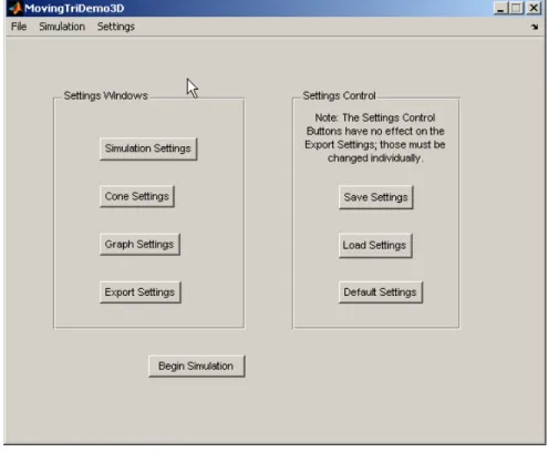
Real-life moored cones in ice can experience a wide range of conditions, so many aspects of MTD3D are variable, and these changes can be made via the settings windows. There are five windows, organized by category: Simulation, Cone, Graph, Export, and Mooring. To open one of these windows, click on one of the buttons
contained inside in the “Settings Windows” panel, which is located on the left side of the start-up window [Figure 1]. Alternatively, click on “Settings” in the menu bar at the top of the start-up window, and then click on the category whose settings you want to adjust. The Mooring settings are not available from the menu bar.
3.2.1 Simulation settings window
The Simulation Settings window [Figure 2] controls the primary variables that govern the simulation engine itself, as well as how the data is presented as it is being generated. The following options are available:
Simulation Characteristics – A panel of 5 variables used to control the Simulink model constants. The variables available are the mass of the cone, the mass of the ice, the coefficient of ice friction, the spring constant, and the acceleration due to gravity, all in SI units. The defaults are 25000, 8000, 0.5, 1 x 10⁶, and 9.81,
respectively.
Simulation Length – The total time period to be simulated, in seconds. Depending on other settings, the program may take more or less time to actually produce the data. In general, the time to produce the data is directly proportional to the simulation length. Default is 10.
Time Increment – The sample period, in seconds. A small increment will take longer to simulate than a large one, since more data is generated over the same time period, but the results will be more accurate and continuous. In the case of a Real Time simulation, the Time Increment is also the pause used in between
calculations. Default is 1.
Initial Position (m) – Three edit boxes to determine the initial position of the moored cone in three-dimensional space. The X and Y co-ordinates refer to the initial position of the centre of the circle face in the horizontal plane, while the Z co-ordinate determines the initial vertical displacement of the circle face of the cone. Default is (0, 0, 0), i.e. at the origin.
Simulation Speed – Determines whether or not a simulation is calculated as fast as the program is able. “Real Time” implements pauses to simulate real time, while “Full Speed” removes any pausing. Default is “Full Speed”.
NOTE: “Real Time” functionality has been removed. There is no check for it so all simulations are executed at full speed. It was found that many simulations were taking close to real time, or even longer, negating the need for the option to implement a pause.
Figure 2: Simulation Settings window
To accept changes and return to the start-up window, press “OK”. To discard changes and return to the start-up window, press “Cancel” or click on the ‘x’ in the top right corner.
3.2.2 Cone settings window
The Cone Settings Window [Figure 3] allows the user to specify the size of the moored cone in the simulation, and how it is plotted on screen. The options are as follows:
Cone Height (m) – The height of the conical component, in metres. A cone with a large height will appear larger on-screen. Typically, moored conical structures have their tip pointing downwards, so to display a cone pointing up a negative value is
required. Default is 0.5.
Cone Radius (m) – The radius of the conical component, in metres. A cone with a large radius will appear wider on-screen Default is 1.
Cylinder Height (m) – The height of the cylindrical component, in metres. When positive values are used for both the cylindrical and conical components, the cylinder will be built leading down from the cone. Default is 0.5.
Cylinder Radius (m) – The radius of the cylindrical component, in metres. Default is 0.5.
Display as 3d Cone – A checkbox controlling whether or not the cone is rendered in three dimensions. If left unchecked, a simple 2-d triangle will appear on-screen. Checking this box will result in a 3-d cone being plotted with the appropriate dimensions. Default is checked.
Cone Colour – Three edit boxes controlling the red-green-blue (RGB) values of the displayed cone or triangle. Each value must be between 0 and 1 inclusive; values greater than 1 or less than 0 are replaced by the previous, correctly entered value. Adjusting these three values provides a lot of flexibility in choosing a desired colour, especially when using decimal values. This table describes the RGB values for common colours:
R G B Colour 0 0 0 Black 0 0 1 Blue 0 1 0 Green 0 1 1 Cyan 1 0 0 Red 1 0 1 Magenta 1 1 0 Yellow 1 1 1 White Default is (1, 0, 0), i.e. Red.
Display Water Surface – A checkbox controlling the display of a simple blue surface representing the ocean. Checking this box plots the surface. Default is unchecked.
NOTE: The water surface will not display if “Dynamic Axes” is selected from “Graph Settings”. This is because the axis limits from “Constant Axes” are used to determine the area plotted.
Figure 3: Cone Settings window
To accept changes and return to the start-up window, press “OK”. To discard changes and return to the start-up window, press “Cancel” or click on the ‘x’ in the top right corner.
3.2.3 Graph settings window
The Graph Settings window [Figure 4] provides plotting options for when a simulation is running. These options are:
Plot during Simulation – A checkbox controlling whether or not the simulated cone is actually displayed while a simulation takes place. Checking the box results in a plotted cone or triangle, depending on the “Display as 3d Cone” option in Cone Settings. The data will be available for post-processing regardless of the existence of the displayed plot. Default is checked.
TIP: To allow a simulation to run as quickly as the engine can calculate, uncheck this box and select “Full Speed” for “Simulation Speed” under Simulation Settings. The program skips the generation of the visual cone object entirely and does not need to worry about re-plotting. Alternatively, leave the box checked if the user plans to monitor the simulation as it takes place, in order to have a general feel for the overall movement of the cone.
NOTE: This box must be checked to if the user intends on generating an AVI video file, or else the video will not appear to be very interesting since there will be nothing generated to view on-screen.
Axes Limits – Determines the way in which the limits of the three co-ordinate axes are calculated. “Constant Axes” uses the six accompanying edit boxes to define the minimum and maximum values of the axes so that they do not change during a simulation. It is not possible to define a minimum limit greater than the maximum, or a maximum limit less than the minimum. “Dynamic Axes” re-defines the axes limits every time the cone or triangle is redrawn. Default is “Constant Axes”, with minimum and maximum values of –5 and 10 for each axis, respectively.
TIP: “Dynamic Axes” is not an ideal choice, since the cone or triangle will appear to remain stationary while the axes adjust. Use “Constant Axes”, particularly when creating an AVI video file. If the user believes the plotting cone will not stray far from its initial position, the axis limits can be set to be fairly close to the cone itself, allowing a clear visualisation of cone movement.
Figure 4: Graph Settings window
To accept changes and return to the start-up window, press “OK”. To discard changes and return to the start-up window, press “Cancel” or click on the ‘x’ in the top right corner.
3.2.4 Export settings window
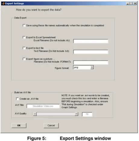
The Export Settings window [Figure 5] controls the ways in which the simulation data is converted for later use. It appears in two different contexts: from the start-up window,
and immediately after a simulation has completed. The differences are explained for the individual settings:
Save using these filenames automatically when the simulation is completed – A checkbox to determine whether the chosen spreadsheet, text file, and/or figure names are used to automatically save the data when a simulation has finished. Checking the box will automatically save the data using the remaining
configurations. This checkbox is not enabled after the corresponding simulation. Also, this checkbox has no effect on AVI video generation settings. Default is un-checked.
NOTE: Even when automatically saving, the Export Settings window will still appear immediately after a simulation. The data will have already been saved, but the user is given the opportunity to export the data again using different filenames.
Export to Excel Spreadsheet – A checkbox to determine whether the simulation data is exported to an Excel spreadsheet. Columns will be labelled for time in seconds and for the three co-ordinate axes in metres. There is an accompanying edit box to provide a filename. The ‘.xls’ suffix will be applied automatically so do not include it in the filename. If a name is provided the Excel file will be saved in the working directory. If no name is provided then Microsoft Excel will open with the simulation data entered, and the user can then specify a filename and folder to save to via the Excel interface. Default is un-checked.
NOTE: If the specified Excel filename already exists in the working directory, there will be a prompt to over-write the file. This feature does not apply to the other methods of data export.
Export to text file – A checkbox to determine whether the simulation data is exported to a simple text file. The columns will not be automatically labelled, but in order from left to right they are time and the x-, y-, and z-co-ordinates, respectively. There is an accompanying edit box to provide a filename. The ‘.txt’ suffix will be applied automatically so do not include it in the filename. If a name is provided the text file will be saved in the working directory. If no name is provided the text file will be saved in the working directory as simply ‘.txt’. Default is un-checked.
NOTE: If the specified text filename already exists in the working directory, the file will be over-written automatically. There will be no prompt to over-write the file.
Export to figure file – A checkbox to determine whether the final view of the plot is exported as an image file. There is an accompanying edit box to provide a filename, and a dropdown list to select a figure format. Supported formats are .png, .bmp, .jpg, and .tif. The appropriate suffix will be applied automatically so do not include it in the filename. If a name is provided the image file will be saved in the working directory. If no name is provided the image file will be saved in the working directory as simply ‘.<FORMAT>’. Default is un-checked.
NOTE: If the specified image filename already exists with the same format in the working directory, the file will be over-written automatically. There will be no prompt to over-write the file.
Create an AVI file – A checkbox to determine whether an AVI video file will be
generated. If checked, the AVI file will be created using the simulation plot view. This checkbox is not enabled after the corresponding simulation. Each time the cone or triangle is redrawn a frame will be captured for use in the video. The frames per second rate (fps) will be 1/Increment, adjusted in “Simulation Settings”. There is a slider and edit box to adjust video quality, from 0 to 100. A higher
number creates a higher-quality video with a larger file size. There is an
accompanying edit box to provide a filename. While it is not necessary to include the ‘.avi’ suffix, doing so will not be a problem. The video will be saved in the working directory. If no name is provided the file will be saved as ‘.avi’. Default is un-checked with a quality value of 75.
NOTE: Do not change windows during a simulation if a video is being generated. The video will capture whatever is onscreen over a specific region of the plotting window, including the interfaces of other programs. Screensavers or turning the monitor off will not disrupt the video.
NOTE: If the specified video filename already exists in the working directory, the file will not be over-written. Rather, a video will be generated but not saved.
NOTE: If a video is being created, the frames need to be captured within the simulation loop. It is because of the computational resources required that the option to build a video must be chosen before the simulation takes place. Building a video anyway and choosing to save it afterwards is not an efficient use of
Figure 5: Export Settings window
To accept changes and return to the start-up window, press “OK”. To discard changes and return to the start-up window, press “Cancel” or click on the ‘x’ in the top right corner. The program will proceed to post-simulation processing when the Export Settings window appears after a simulation.
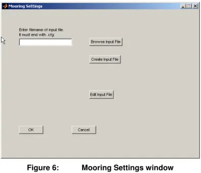
3.2.5 Mooring settings window
The Mooring Settings window [Figure 6] has no effect whatsoever on any other
component of MTD3D. It was created to demonstrate the possibility of using text files to write data to and read it from. In this case a settings file is considered for an in-house IOT software program (Stanley and Lau, 2005), written in Fortran. The mooring system program requires an input file with a specific format. The Mooring Settings window allows the user to create an appropriate file by entering the necessary information in the user interface. The options available are:
Browse Input File – A button to search the file directory for a ‘.cfg’ input file. There is an accompanying edit box to specify a filename or to enter a filename directly.
Create Input File – A button to open the Mooring System Configuration Creation window [Figure 7] to create a new input file.
Edit Input File – A button to open the Mooring System Configuration Creation window and load into it the input file specified in the “Browse Input File” edit box. The file can be edited and saved, using the same name or a different one.
Figure 6: Mooring Settings window
To accept changes and return to the start-up window, press “OK”. To discard changes and return to the start-up window, press “Cancel” or click on the ‘x’ in the top right corner.
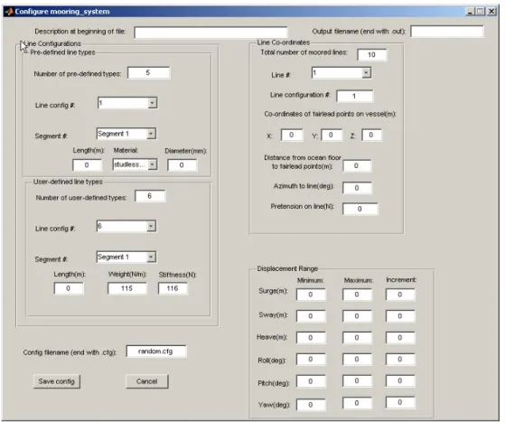
3.2.6 Configure mooring_system window
The Mooring System Configuration Creation window [Figure 7] is not an actual settings window, but combined with the Mooring Settings window [Figure 6] it demonstrates how models could be integrated with future software iterations. Its controls deal with the settings necessary for the mooring_system program.
Description at beginning of file – A string used to describe the file. Any character can be used; the only limitation is that it must be a single-line string.
Output filename – A name for the filename to use for the program output. It must end with ‘.out’.
Number of pre-defined types – The number of pre-defined mooring line configurations the user would like to use. When this number is changed, the dropdown menu for the current configuration to edit changes appropriately. Each line type has three segments, each of which has their own length, material, and diameter.
Number of user-defined types – The number of user-defined mooring line configurations the user would like to use. When this number is changed, the dropdown menu for the current configuration to edit changes appropriately. User defined
Each line type has three segments, each of which has their own length, weight, and stiffness.
Total number of moored lines – An edit box to specify how many lines are being attached to the structure. A dropdown menu lets the user specify which line they are editing at a given moment. Each line can have its own line type value (each of which is defined in the pre-defined and user-defined panels), fairlead point on the vessel, distance from ocean floor, azimuth, and pretension.
Displacement Range – The range in the six degrees of freedom over which the
simulation is calculated. A minimum, maximum, and increment can be specified for each degree of freedom (surge, sway, heave, roll, pitch, and yaw).
Figure 7: Mooring System Configuration Creation window
To rewrite the input file and return to the Mooring Settings window, press “Save config”. To discard changes and return to the Mooring Settings window, press “Cancel” or click on the ‘x’ in the top right corner.
3.3 Load and Save Options
In order to keep track of the settings configurations most commonly used, there are options to save and load settings. It is also possible to reset all settings to their program defaults. The buttons for these options are placed on the “Settings Control” panel on the right side of the start-up window [Figure 1]. Alternatively, click on “File” in the menu bar at the top of the start-up window, and then click on the appropriate button to Load, Save, or Default the settings.
3.3.1 Save settings
Clicking on the Save Settings button or selecting “Save Settings” from the File menu will open a dialogue box to enter a name to save the current settings with. The file will be saved as a rich text file in the working directory. To ensure compatibility, append the ‘.ini’ suffix to the filename. Press “OK” to save.
Once the file has been saved, it can be opened with Notepad, WordPad, Microsoft Word, or any other standard word processor.
3.3.2 Load settings
Clicking on the Load Settings button or selecting “Load Settings” from the File menu will open a window to search for a settings file. By default, the first directory is the working directory, but the user is free to navigate to any folder where a settings file may exist. The browser is automatically filtered for .ini files, and it is recommended to not change the file type.
Ensure the file you load is a correct settings file. If it is not, it will not load properly and MTD3D may need to be restarted. The safest practice is to only load settings files that have been created via the “Save Settings” button.
3.3.3 Default settings
Clicking on the Default Settings button or selecting “Default Settings” from the File menu will load a pre-specified configuration. The default values are those described for each setting in Section 3.2.
3.4 Conducting a Simulation
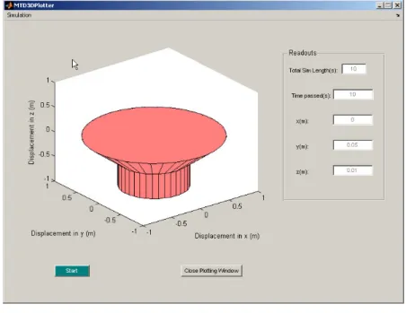
From the start-up window [Figure 1], press the “Open Sim Window with Current Settings” button or click on “Begin Simulation” from the Simulation menu. The
MTD3DPlotter window [Figure 8] will open with the settings chosen from the start-up window.
Figure 8: MTD3DPlotter window
To begin the simulation, press the “Start” button in the bottom left corner. If the “Plot during simulation” checkbox was checked (see Section 3.2.3) then the plot will appear onscreen in the plot area. As the calculations are performed, the plot will be updated to display the location of the moored cone or triangle. The “Readouts” panel displays the simulation length, the current time being plotted, and the current location of the cone in three dimensions. If no plot is being drawn, it is likely that the simulation will be
progressing too quickly for the readouts to display any values.
NOTE: Do not change windows during a simulation if a video is being generated. The video will capture whatever is onscreen over a specific region of the plotting window, including the interfaces of other programs. Screensavers or turning the monitor off will not disrupt the video.
3.5 Post-Processing a Simulation
When a simulation completes, the generated data is available to be explored and analyzed. MTD3D provides the user with many methods in which to process this information.
The simulation itself is a generated matrix of co-ordinates in the x, y, and z directions, as well as a column specifying time. This data can be displayed via AVI movies and 2-d plots, and can be stored via spreadsheets.
3.5.1 Initial data export
As soon as a simulation is finished the Export Settings window will open. All of its features are described in Section 3.2.4.
If the data is exported to an Excel spreadsheet, any spreadsheet software that can open it will be able to view the raw results and manipulate them in any way the software will allow. This may include summaries, custom graphs, etc.
Users without excel who still wish to export the raw data will find it useful to export the data to a text file. Text files can be read in WordPad, Microsoft Word, or any other word processor. NotePad is not recommended because it does not display the text correctly. A generated AVI video file can be opened for playback using Windows Media Player on any computer with the XVid codec.
3.5.2 Additional plot analysis
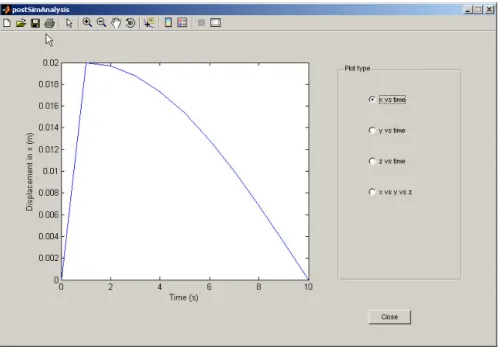
When the Export Settings window is closed the Post-Processing window will appear [Figure 9]. A labelled plot displays the displacement versus time for the x-axis. Radio buttons allow changing to a different axis, or to trace the displacement off all three axes together. The user is free to edit this plot in many respects, including label, title, colour, scale, legend display, and more. Using the figure toolbar, the plot can be rotated, zoomed, and otherwise manipulated. Pushing the “Close” button will return the user to the MTD3DPlotter window [Figure 8]. From there, press “Start” to run the simulation again with the same settings, or press “Close Plotting Window” to return to the start-up window [Figure 1].
Note: The radio buttons have no effect. The Simulink model generates data in one dimension only, so the functionality of the radio buttons was removed.
3.6 Quitting MTD3D
While it is possible to quit MTD3D during a running simulation, it is not recommended as errors may occur. It is best to close the program before or after simulations have
completed, beginning with any settings windows. Here is the recommended order in which to close program windows:
1. Any settings windows 2. Post-Processing window 3. MTD3DPlotter window 4. Start-up window
If the non-compiled version is being run, Matlab must be open for MTD3D to keep running. Closing Matlab will close MTD3D. When quitting, close Matlab after all MTD3D windows have been closed.
4.0 FREQUENTLY ASKED QUESTIONS
Q.Why does the program only use 25% or 50% of my computer processing power? How can I make it use 100% of my computer’s resources?
A. MTD3D is built upon the Matlab calculating engine, which is not designed to take full advantage of multi-threaded and dual-core processors. When using one of these types of processors to run a single instance of a Matlab program, it is not possible to use 100% of the computer’s processing speed. If you are able to open multiple instances of Matlab (depending on your license), you can open as many copies of MTD3D
separately and thus use up to 100% of the computer’s resources.
Q.I want to know more about the code used to program MTD3D and its graphical user interface. Where can I find this information?
A. The graphical user interface (GUI) was created in Matlab version 7 Release 14. This User’s Manual was created to provide all the necessary details to use the interface without needing to work with the underlying code. The functions in MTD3D are
described in Appendix A. For full details on how the code is structured, please refer to “GUI Programmer Manual for OSIS (Ocean-Structure Interactions Simulator) – Version 1” (Noel and Lau, 2006).
Q.What is OSIS and what does it have to do with MTD3D?
A. A point came in the development of MTD3D where it was realised that the design restricted the user in some respects. The GUI was re-created and designed to be much more versatile and intuitive. This GUI was named the Ocean-Structure Interactions Simulator (OSIS). Its documentation includes the history of the development of MTD3D, since they are, practically speaking, one and the same. OSIS is the newer version of MTD3D, and much of the code was re-used for it.
Q.I am trying to generate an AVI video file but I get an error when trying to run the simulation. What am I doing wrong?
A. MTD3D uses the Xvid codec for video compression. You need this codec in order to generate and view AVI files for this program. The Xvid codec preserves quality while keeping file sizes small. It is available for free as a download from
www.xvidmovies.com/codec.
Q.I have created an AVI video file, and I sent it to somebody else, but they are unable to view the file on their media player. Why not?
A. MTD3D uses the Xvid codec for video compression. You need this codec in order to view any AVI file made by this program. The Xvid codec preserves quality while keeping file sizes small. It is available for free as a download from www.xvidmovies.com/codec.
Q.A simulation is running and I cannot see any values on the readouts. Why is this?
A. If you are running a full speed simulation, and you have the “Plot during Simulation” checkbox un-checked, it is possible for the simulation to be calculating too quickly for the values to display. Run the simulation in “Real Time” or check the plotting box in order to view the data as it is generated.
Q.I created an AVI video file but when I watch it I see other windows that I had opened while the simulation was running. How can I fix this?
A. MTD3D is built upon the Matlab engine, which generates video by capturing what is on-screen. In order to generate a video without any “disturbances”, it is important to not try to change windows throughout the length of the simulation.
5.0 REFERENCES
Noel, A., 2006. “Graphical User Interface Development for Ocean Models”, NRC/IOT Report SR-2006-04, Institute for Ocean Technology, National Research Council of Canada, St. John’s, NL.
Noel, A., and Lau, M., 2006. “GUI Programmer Manual for OSIS (Ocean-Structure Interactions Simulator) – Version 1”, NRC/IOT Report LM-2006-02 (Protected), Institute for Ocean Technology, National Research Council of Canada, St. John’s, NL.
Stanley, J., and Lau, M., 2005. “Spread Mooring: Software for Mooring System Load Analysis”, NRC/IOT Report LM-2005-03, Institute for Ocean Technology, National Research Council of Canada, St. John’s, NL.
Appendix A
MTD3D uses the Matlab programming language. It is assumed that the reader has an understanding of how the language works, including functions, handles, callbacks, file interfacing, and plotting. The functions described here are those external to the GUI-specific M-files, since they can be used for other applications. Please refer to the OSIS documentation for explanations of Matlab components, and how GUIs are created. The functions are listed alphabetically.
[xpts, ypts, zpts, faces] = buildMooredCone(r1, d1, r2, d2, res)
Inputs:
r1 – Radius of the conical component
d1 – Depth of the conical component (positive value for a cone pointing down) r2 – Radius of the cylindrical component
d2 – Depth of cylindrical component
res – resolution, in degrees, of the structure Outputs:
xpts – column of x co-ordinates of the vertices ypts – column of y co-ordinates of the vertices zpts – column of z-co-ordinates of the vertices
faces – a matrix of all faces of the moored conical shape. Each row defines what vertices are used for a face.
Description:
This function was designed with the ‘patch’ plotting function in mind. It uses the input size variables to determine where all of the vertices would be located. Vertex n’s location would be defined by the nth row of the ‘xpts’, ‘ypts’, and ‘zpts’ columns.
The function will assign defaults if there are fewer than 5 arguments passed in. If there are fewer than 5 it will assign 10 to ‘res’, if there are fewer than 4 it will assign 0.5 to ‘d2’, if there are fewer than 3 it will assign 0.5 to ‘r2’, if there are fewer than 2 it will assign 0.5 to ‘d1’, and if there are none it will assign 1 to ‘r1’.
The original version of this function was entitled ‘buildCone’, and it only determined the points and faces of a simple cone. This version added the points for the cylindrical component (two circles), the faces for the cylindrical component sides, and a face on either end to enclose the object. In order to do this properly, the resolution is used to determine how many points are in each circle. This number of points is the same for each circle: the circle at the wide cone-end, the circle where the cone and cylindrical components meet, and the circle at the other cylinder end. While loops build the four-point faces for the conical component and then the cylindrical component. In order to add the faces at the ends, the matrix of faces must be appended with NaNs so that the number of columns matches the number of points in each circle. The rows for the end faces list every vertex in the respective circle.
Before calling the patch function, the x, y, and z columns must be combined into a single, 3-column matrix. This is intentional so that each column may have a different displacement added before being combined.
[X Y Z C] = buildSurfPoints(xmin, xmax, ymin, ymax)
Inputs:
xmin – minimum x-value in the axes xmax – maximum x-value in the axes ymin – minimum y-value in the axes ymax – maximum y[value in the axes Outputs:
X – 2x2 matrix of x co-ordinates Y – 2x2 matrix of y co-ordinates Z – 2x2 matrix of z co-ordinates C – 2x2 matrix colour map Description:
This function is a preparation function for a surf plot, and it is much simpler than preparing for a patch plot. The resulting matrices are used as input arguments to the surf command to create a water surface in the plotting window.
The axis limits are used to make a mesh grid of x and y points. This grid’s co-ordinates become the ‘X’ and ‘Y’ matrices. The ‘Z’ matrix is created as a 2x2 matrix of random points, all with values near –0.5. The randomness creates a slight tilt for the “water” surface. The colour map created is [-2 0; -2 -2], which appears as a solid blue when the ‘CLim’ property of the axes is set to [-2 2].
buildToolbar(handles)
Inputs:
handles – the handles structure of the post-processing GUI Outputs:
NONE Description:
This function was called by the opening function of the Post-Processing GUI of MTD3D, however any GUI can readily use it. It creates a toolbar to go along the top of the calling figure with tools for use with a plotted graph.
Each icon in the toolbar has a solid colour, defined by a 20x20x3 matrix, and a tool tip string that appears when the mouse cursor is held over it, telling the user what the icon is able to do.
The callbacks for each icon were coded as strings because they had to be included with the call to create the button. Some of the callbacks were quite lengthy and so were stored to a large string beforehand. Four of the tools, being pan, zoom, rotate, and data cursor, are mutually exclusive, so turning on one means ensuring the other three are turned off. The save button needed to include the call to the “uiputfile” function and specify the file types available for saving the figure.
clearAxes Inputs: NONE Outputs: NONE Description:
This is a very simple function used to clear the current axes and rewrite the labels for the axes. The function stores the axis limits for the current axes, clears the axes so that nothing is plotted, restores the axis limits, and writes standard labels for the axes.
Assuming the labels were already there, the function gives the effect of erasing the plots from a graph while keeping the graph intact.
editAllSettings(handles, varargin)
Inputs:
handles – structure of handles of the MovingTriDemo3D GUI varargin – a variable-sized cell array of input arguments Outputs:
NONE Description:
This function is considered obsolete, even for MTD3D itself, but it is still functional. A callback from MTD3D can call this function and pass it the GUI handles and a list of arguments to replace the current settings. The handles structure is then saved.
This function requires that the input arguments be in a very precise order because the order of arguments in ‘varargin’ is used to fill the handles’ fields. There also must be enough input arguments for all of the necessary fields. 21 arguments are needed in addition to the handles structure, and they are, in order:
1. doPlot (Boolean) 2. dynamicAxes (Boolean) 3. xmin (double-precision) 4. xmax (double-precision) 5. ymin (double-precision) 6. ymax (double-precision) 7. zmin (double-precision) 8. zmax (double-precision) 9. simlength (double-precision) 10. increment (double-precision) 11. realtime (Boolean) 12. xorig (double-precision) 13. yorig (double-precision) 14. zorig (double-precision) 15. coneHeight (double-precision) 16. coneRadius (double-precision) 17. cylinderHeight (double-precision) 18. cylinderRadius (double-precision) 19. is3d (Boolean)
20. coneColour (1x3 matrix; all values between 0 and 1 inclusive) 21. plotWater (Boolean)
This method for loading settings was replaced by a function to load a text file of settings and immediately store the data (“settingsFileWrite”). However, the function is still used for loading a set of pre-defined default settings since a default settings file was not created. Note that the “realtime” variable is not implemented anymore.
points = movePoint(xpts, ypts, zpts, xDis, yDis, zDis)
Inputs:
xpts – column of x co-ordinates of the vertices ypts – column of y co-ordinates of the vertices zpts – column of z-co-ordinates of the vertices
xDis – amount by which to translate the x co-ordinates yDis – amount by which to translate the y co-ordinates zDis – amount by which to translate the z co-ordinates Outpus:
points – an n x 2 or n x 3 matrix of two- or three-dimensional points Description:
By design this function uses the output columns from the buildMooredCone function to create the vertices matrix required by the patch plot. While combining the columns, it is able to add a scalar displacement to each one.
This function is able to accept four arguments, which it treats as ‘xpts’, ‘ypts’, ‘xDis’, and ‘yDis’. In that case the ‘z’ column will be empty. Also, if there are only three input
arguments, the displacements are assumed to be zero. Checks are made to ensure that the columns are all of the same size, which they must be in order to horizontally
concatenate.
The displacement of the columns and concatenating them together is performed in a single line of call that calls the “horzcat” function.
handle = plotCone(vertices, faces, colour)
Inputs:
vertices – an n x 2 or n x 3 matrix of point co-ordinates
faces – a matrix specifying which points connect to build each face colour – a 1 x 3 matrix defining the colour
Outputs:
handle – handle to the plotted object Description:
This function calls the “patch” function with the input arguments and returns the handle to the created plot object. The name “plotCone” is misleading because it is able to plot any two- or three-dimensional object given the proper inputs, however it was initially created to plot the simple cone for MTD3D.
The “patch” function can be called in two different ways; the one used here was to provide a matrix of vertices, where each row is the x and y or x, y, and z co-ordinates of a vertex, and a matrix of faces, where each row defines the vertices that combine to create a face. The ‘vertices’ used is the output from the “movePoint” function and the ‘faces’ matrix is the fourth output argument from the “buildMooredCone” function. Once the object is created by the “patch” function, the returned handle can be used to identify the existence of the object in order to delete it. This capability is necessary when
multiple graph objects are onscreen at once but only one needs to be deleted. The ‘colour’ vector is used to define the face colour of the plotted object, where the three values in the vector correspond to RGB values and must all be in between zero and one inclusive. It is also possible to provide a single number to define the colour, in which case its value must lie within the colour limits of the given axes. Thirdly, a string can be used to define the colour; common colours can be chosen in this manner, such as ‘black’. The edge colour of the plotted object is black no matter what the value of ‘colour’ is.
saveOutput(Data, Axes, auto, handles)
Inputs:
Data – matrix of data to store as output Axes – handle of the plot to export
auto – Boolean to check if the call being made is for auto-saving handles – structure of handles from the calling function
Outputs: NONE Description:
This function exports the data matrix in the requested formats. When saving is to occur, the ‘handles’ structure is used to decide what formats are filenames are to be used. It is called by the simulation function after the ‘Data’ matrix has been created.
If ‘auto’ is true then there is no user interaction, else the “Export Settings” GUI opens for the user to define how the ‘Data’ matrix and ‘Axes’ figure will be exported. Excel
spreadsheets are created using the “xlswrite1” function, with default headings used for every column. Text files are created using “dlmwrite”, given a filename, ‘Data’, and a tab delimiter (should not be opened in Notepad). When capturing a figure, the “getframe” function captures what is on the ‘Axes’ plot and then “imwrite” is used with the correct components of the frame to create the figure.
A number of aspects of this function can be improved. It is not necessary to call the third-party-created “xlswrite1” function, since the default “xlswrite” is sufficient once the data has been combined properly. The “dlmwrite” function is not very robust for creating text files; the “fprintf” method allows much more flexibility. Also, if the “else” component of the function was placed after the “if” statement, it would not be necessary to call the function twice (once for being automatic, and then a second time).
settingsFileRead(fileName, handles)
Inptuts:
fileName – name of the ‘.ini’ settings file to load
handles – handles structure of the MTD3D main window Outputs:
NONE Description:
This function opens a created settings file, reads its contents, stores them to the
MTD3D ‘handles’ structure, and updates the structure. If the provided ‘fileName’ cannot be opened by the “fopen” function, nothing further is attempted. If the file is opened, ‘fid’ is used as a handle to the file in all calls to “textscan”.
By design this function reads files created by the “settingsFileWrite” function, however it is possible for a user to create their own settings files and save them as ‘.ini’ files in Notepad. In this case the order in which the settings are defined must be identical to that of “settingsFileWrite”. There is no limit to the amount of opening comments that can be entered by the user at the beginning of a settings file, however the “equals” sign must not be used, as that is the character used to locate where settings values are. To read values the “textscan” function is used. In each call, it is instructed to read to the next “equals” sign in the file while discarding everything up to it, read and discard the “equals” sign itself, and then read the required value in the correct format. The value is placed into the ‘holder’ variable that can then be referenced to store the value into the appropriate field of ‘handles’. The ‘holder’ variable is a cell array and must be
referenced as such. In the case of extracting the cone colour, the first element of each of the first three cells of ‘holder’ is read. In the case of strings, which are stored as a nested cell array in ‘holder’, ‘holder’ must be referenced twice on separate lines. The “fclose” function closes the settings file before the ‘handles’ structure is updated.
settingsFileWrite(fileName, handles)
Inptuts:
fileName – name of the ‘.ini’ settings file to create or over-write handles – handles structure of the MTD3D main window Outputs:
NONE Description:
This function builds a settings file from the values in the MTD3D ‘handles’ structure. If the provided ‘fileName’ cannot be created or over-written by the “fopen” function, nothing further is attempted. If the file is open, ‘fid’ is used as a handle to the file in all calls to “fprintf”. Please reference “settingsFileRead” for information on how a user can create their own settings files.
“fprintf” is used for all writing in the file. A heading is created that identifies the file as a settings file for MTD3D, and the current date is added. The settings are written by category with an appropriate heading. Each setting is written on its own line with a name for the setting, an “equals” sign, and the value of the setting.
data = simulation(handles)
Inputs:
handles – the handles structure of MTD3DPlotter Outputs:
data – matrix of simulation results Description:
This function is the most important component of MTD3D; it takes all of the settings and runs the actual simulation. It calls most of the other functions to complete various tasks, and once completed ‘data’ is returned for further access.
Upon starting, the function calls “clearAxes” to ensure there are no previously created plots to interfere. The “cputime” is stored to keep track of how long the simulation takes. The “start” and “close” buttons of “MTD3DPlotter” are disabled to prevent interference during a simulation.
The tag of the axes must be set because when a simulation is repeated it is cleared. “hold” is turned on to keep multiple objects in the plot. The AVI video object is then created if required with the specified name, compression, frames-per-second rate, and quality. All simulation data is initialized, including the variables required by the Simulink model. The cone and water points are created if necessary and the water surface is displayed.
During the simulation loop all warnings are suppressed because the Simulink model is known to generate warnings. The time variable, ‘t’, is incremented and used to define the time interval for the Simulink model in the call to the “sim” function. The actual model used is called “surge_force_3.mdl”. Output from the model is used to define the second column of the data matrix.
If plotting, the loop also builds the moored cone with the calculated displacement, deletes any previous displayed object (not the water surface), adjusts the axis limits, and adds a frame to the AVI video. A readout panel is updated to provide the current location of the structure and the amount of simulation time that has passed.
After the simulation loop, an obsolete check is made to check the last error against “invalid handle object.” At one point in development that was an error that consistently appeared but it has since been fixed.
The AVI object is closed so that it can then be accessed. The simulation time is
displayed in the command window of Matlab. The data is saved automatically saved if required, and then the “Export Settings” window is displayed to allow more exporting. The “start” and “close” buttons of “MTD3DPlotter” are enabled, and the ‘data’ matrix is assigned to return.
xlswrite1(m, header, colnames, filename, sheetname)
Inputs:
m – matrix of data to write to file
header – optional string of header information
colnames – optional cell array of strings to use as column headers
filename – optional name of excel file to use for saving. If none is provided then Excel is opened with the contents
sheetname – optional sheet to write the data to. Default is “Sheet1”. The sheet must exist if specified.
Outputs: NONE Description:
This function was not created in-house. Scott Hirsch of The MathWorks developed it, and it was made available on the Matlab user file exchange. It was originally named “xlswrite”, the same name as the default Matlab excel spreadsheet-writing function. A “1” was appended to avoid a warning every time the function was called.
It is recommended to use the default Matlab function, since it provides the same functionality if the user knows how to properly build a cell array.
Appendix B
Development of MovingTriDemo3D, A Software Simulation – Progress Report
B.1.0 Background... 1 B.2.0 Introduction to MovingTriDemo3D ... 1 B.3.0 Visual Layout ... 1 B.3.1 MovingTriDemo3D GUI ... 2 B.3.2 simulationSettings GUI... 2 B.3.3 coneSettings GUI ... 2 B.3.4 graphSettings GUI... 2 B.3.5 exportSettings GUI ... 3 B.3.6 MTD3DPlotter GUI ... 3 B.4.0 Using MovingTriDemo3D... 3 B.4.1 Using the Settings Windows... 4 B.4.2 Video Exporting Details ... 4 B.4.3 Saving and Loading... 5 B.4.4 Known Bugs ... 5 B.5.0 Programming Notes ... 6 B.5.1 Necessary Files... 6 B.5.2 Files Which Do Not Run A Specific GUI... 6 B.5.3 Overhauling the Passing of Data... 7 B.5.4 Re-Organization of GUIs ... 7 B.6.0 Future Considerations to Implement ... 8
TABLE OF FIGURES
Figure B-1: MovingTriDemo3D GUI...B-9 Figure B-2: simulationSettings GUI ...B-9 Figure B-3: coneSettings GUI...B-10 Figure B-4: graphSettings GUI ...B-10 Figure B-5: exportSettings GUI ...B-11 Figure B-6: MTD3DPlotter GUI...B-11
DEVELOPMENT OF MOVINGTRIDEMO3D, A SOFTWARE SIMULATION – PROGRESS REPORT B.1.0 BACKGROUND
A software development project is in place to model the dynamic response of a moored conical structure in ice. A graphical user interface (GUI) must be designed
simultaneously to allow a user to interact with the simulation model. MovingTriDemo3D is being developed as a proof of concept GUI to showcase the functions that would be desired in the final product. This GUI is being created in Matlab, so MovingTriDemo3D is also being used as a practical learning tool to become familiar with the Matlab environment.
B.2.0 INTRODUCTION TO MOVINGTRIDEMO3D
MovingTriDemo3D is named as such to be a condensed form of Moving Triangle Demonstration in Three Dimensions. As a program, MovingTriDemo3D has two main purposes. The first is to visually display a cone moving along a calculated path in 3-D space. When the cone is re-drawn, previous plots are erased so one can follow the kinetics of the cone on the graph. The movement is calculated in simulated real-time, such that there is a constant pause in between calculations. Plotting continues until a specified period of time has passed.
The second purpose of the software is to export the collected data in various forms for further review and analysis. It is desired to have both numerical data, for comparing with relevant mathematical models, and visual data, to easily see any phenomena that may occur under specific conditions.
Please note that all information recorded here is subject to change as this software is being continuously modified. There are bugs possible at any given time, and the ones listed here are those observed as of the time of this writing. Future reports may include fixes or perhaps even newly discovered problems.
B.3.0 VISUAL LAYOUT
MovingTriDemo3D is a simple application with multiple GUIs. There are six GUIs currently implemented, entitled “MovingTriDemo3D”, “MTD3DPlotter”, “exportSettings”, “coneSettings”, “graphSettings”, and “simulationSettings”. All settings GUIs have “OK” and “Cancel” push buttons, along with the others mentioned in this section. Further details on how these GUIs interact are provided in Section 4.
B.3.1 MovingTriDemo3D GUI
The start-up GUI for the software is “MovingTriDemo3D” [Figure 1], so it is the one to be opened in order to use the other GUI’s properly. It contains nine menu options
accessible from the menu bar and eight push buttons. The menu options are grouped into “File”, “Simulation”, and “Settings”. The only menu option without a corresponding button is the “Close” option, under “File”, which exits the program. All of the other menu options provide the same functionality as push buttons of similar name, so only the push buttons remain to be described.
“Save Settings” writes all of the current settings to a rich text format (.rtf) file with a name specified by the user. “Load Settings” prompts the user to retrieve an appropriate .rtf-file from which to load settings. “Default Settings” resets settings to pre-defined values. “Simulation Settings”, “Cone Settings”, “Graph Settings”, and “Export Settings” load the “simulationSettings”, “coneSettings”, “graphSettings”, and “exportSettings” GUIs, respectively. These settings GUIs each handle a specific category of settings, as implied by the respective names. “Begin Simulation” calls the “simulation” function.
B.3.2 simulationSettings GUI
The “simulationSettings” GUI [Figure 2] allows the user to adjust the duration of a simulation and the time at which to sample via edit boxes. Two radio buttons provide a choice between a “Full Speed” or “Real Time” simulation, which only affects how quickly the results are generated. Three edit boxes specify the initial x-y-z co-ordinates of the plotted cone.
B.3.3 coneSettings GUI
The “coneSettings” GUI [Figure 3] provides options to manipulate the cone that will be simulated. Edit boxes let the user specify the radius and depth of the cone. If the “Display as 3-d Cone” checkbox is unchecked, a 2-d triangle with a constant size is drawn instead.
B.3.4 graphSettings GUI
The “graphSettings” GUI [Figure 4] allows the user to define the limits for the axes in the simulation plot. Radio buttons entitled “Constant Axes” and “Dynamic Axes” toggle between user-defined axis limits and limits which are re-defined every time a cone is drawn, respectively. Six edit boxes define the minimum and maximum values of x, y, and z, assuming “Constant Axes” is selected.
B.3.5 exportSettings GUI
The “exportSettings” GUI [Figure 5] provides numerous options for data export. Depending on when the GUI is opened, some options will not be available (this is described further in Section B.4). A checkbox is provided for every type of export, including to an Excel file, a text file, a picture file, and a video file. There is a checkbox to allow automatic saving to particular filenames once a simulation has completed. Edit boxes allow the user to provide filenames for the different files formats. In the case of exporting a picture, a dropdown list displays the file formats available to export to. In the case of exporting a video, there is a slider and accompanying edit box to adjust the quality.
B.3.6 MTD3DPlotter GUI
The GUI that displays the plot and simulation results as they are calculated is
“MTD3Dplotter” [Figure 6]. A set of axes displays the plot with visual axis increments and labels. Disabled edit boxes display the total length of the simulation, the amount of time that has passed, and the current co-ordinates of the cone.
This GUI also has four push buttons. “Stop” halts the plotting loop before it reaches the end of the specified period of time. “Clear Axes” erases all points currently plotted on the graph. “Save Sim Data Now” pauses a simulation for data export. “Close Plotting Window” closes the GUI.
B.4.0 USING MOVINGTRIDEMO3D
Currently, the functions for plot generation are contained directly inside the loop that creates the plot. They are easy to adjust inside the m-file entitled “simulation.m”, and as of this moment are set to x = 0.02*cosd(10*t), y = 0.05*sind(10*t) - 0.05*cosd(10*t^2), and z = 0.01*sind(10*t), where t is the time which has passed since the beginning of the plot. These equations generate an interesting oscillating effect without a significant amount of translation, so the axes can be kept close to the cone. The cone itself has vertices that are calculated at the beginning of the simulation function, but the actual conical object is generated within the loop, taking into account the displacement along each axis. The x-, y-, and z-points define the location of the centre of the circle face of the cone. By default, the cone is pointing downwards to agree visually with a moored conical structure. The graph is labelled to have displacement measured in metres (an arbitrary choice) along the x- and y-, and z-axes.
In the case of a non-3-D plot, the marker is an upside-down triangle, used to represent a conical structure in 2-D. At this moment it has a default size, independent of the radius and height settings chosen.
B.4.1 Using the Settings Windows
As the titles of the settings windows have already been discussed (see Section B.3), the following paragraphs do not specify the exact GUI where each of the options can be found. It should be noted that whenever a setting is adjusted, the “OK” button for the respective window must be pressed. Pressing “Cancel” resets settings to what they were before the respective window was opened.
The default time settings are for a ten second simulation with one-second intervals. The axes are set to remain constant, with minimum and maximum values of -5 and 10, respectively, in all three directions. The simulation speed is set to real-time, so the increment is used to pause the loop and to augment the time variable. A full-speed simulation would omit the pause. By default, the initial co-ordinates are at the origin. As of this moment, changing the cone height and radius affects only the visual size and not the calculations for displacement.
Data can be exported to an excel spreadsheet, a text file, an image file, and a video file in the working file directory. If a video file is to be created, its checkbox must be chosen and a name given before running the simulation. This is because a video file must be built as the simulation progresses, and doing so unnecessarily consumes a significant amount of computing power. The user will be warned of over-writing a file ONLY in the case of an excel spreadsheet with the same name. If the excel box is checked and there is no filename given, Excel will open and the spreadsheet can be saved with a name from there. Although the variables for the plotting themselves are continuously being over-written, and technically each cone drawn is its own individual plot, a matrix is built inside the loop to keep track of all calculated values for x, y, z, and t (time) in
chronological order. This matrix is what is sent to the xlswrite1 and dlmwrite functions. If the data is not saved at all then the numerical data of the simulation is lost. All that remains is the image of the graph on-screen. Exporting to an image file currently captures the graph itself and not its labels. File formats available are Portable Network Graphic (.png), Windows Bitmap (.bmp), Joint Photographic Experts Group (.jpg), and Tagged Image File Format (.tif).
If the user selects to save data automatically, then the exporting of Excel, text, or figure files occur as soon as a simulation ends, using the filenames provided. However, the export window will still open after the automatic saving to allow the user to save the data again using other filenames or formats.
B.4.2 Video Exporting Details
As already noted, in order for a video to be compiled the appropriate checkbox must be selected and a filename given before running the simulation. The inverse of the
increment variable is used to decide the frames-per-second (fps) rate. For example, an increment of 0.04s will result in 25fps. Even at full-speed it takes a while to build a video