Publisher’s version / Version de l'éditeur:
Atmospheric Chemistry and Physics, 9, 4, pp. 1111-1124, 2009-02-16
READ THESE TERMS AND CONDITIONS CAREFULLY BEFORE USING THIS WEBSITE.
https://nrc-publications.canada.ca/eng/copyright
Vous avez des questions? Nous pouvons vous aider. Pour communiquer directement avec un auteur, consultez la première page de la revue dans laquelle son article a été publié afin de trouver ses coordonnées. Si vous n’arrivez pas à les repérer, communiquez avec nous à PublicationsArchive-ArchivesPublications@nrc-cnrc.gc.ca.
Questions? Contact the NRC Publications Archive team at
PublicationsArchive-ArchivesPublications@nrc-cnrc.gc.ca. If you wish to email the authors directly, please see the first page of the publication for their contact information.
Archives des publications du CNRC
This publication could be one of several versions: author’s original, accepted manuscript or the publisher’s version. / La version de cette publication peut être l’une des suivantes : la version prépublication de l’auteur, la version acceptée du manuscrit ou la version de l’éditeur.
For the publisher’s version, please access the DOI link below./ Pour consulter la version de l’éditeur, utilisez le lien DOI ci-dessous.
https://doi.org/10.5194/acp-9-1111-2009
Access and use of this website and the material on it are subject to the Terms and Conditions set forth at
Attribution of projected changes in summertime US ozone and PM2.5
concentrations to global changes
Avise, J.; Chen, J.; Lamb, B.; Wiedinmyer, C.; Guenther, A.; Salathé, E.;
Mass, C.
https://publications-cnrc.canada.ca/fra/droits
L’accès à ce site Web et l’utilisation de son contenu sont assujettis aux conditions présentées dans le site LISEZ CES CONDITIONS ATTENTIVEMENT AVANT D’UTILISER CE SITE WEB.
NRC Publications Record / Notice d'Archives des publications de CNRC:
https://nrc-publications.canada.ca/eng/view/object/?id=7970170e-1159-4a8a-9db6-fe849af48c2f https://publications-cnrc.canada.ca/fra/voir/objet/?id=7970170e-1159-4a8a-9db6-fe849af48c2f
www.atmos-chem-phys.net/9/1111/2009/ © Author(s) 2009. This work is distributed under the Creative Commons Attribution 3.0 License.
Chemistry
and Physics
Attribution of projected changes in summertime US ozone and
PM
2.5
concentrations to global changes
J. Avise1,*, J. Chen1,**, B. Lamb1, C. Wiedinmyer2, A. Guenther2, E. Salath´e3, and C. Mass3 1Laboratory for Atmospheric Research, Washington State University, Pullman, Washington, USA 2National Center for Atmospheric Research, Boulder, Colorado, USA
3University of Washington, Seattle, Washington, USA
*now at: California Air Resources Board, Sacramento, CA, USA **now at: National Research Council of Canada, Ottawa, ON, Canada
Received: 12 June 2008 – Published in Atmos. Chem. Phys. Discuss.: 11 August 2008 Revised: 6 January 2009 – Accepted: 15 January 2009 – Published: 16 February 2009
Abstract. The impact that changes in future climate,
an-thropogenic US emissions, background tropospheric com-position, and land-use have on summertime regional US ozone and PM2.5concentrations is examined through a ma-trix of downscaled regional air quality simulations, where each set of simulations was conducted for five months of July climatology, using the Community Multi-scale Air Quality (CMAQ) model. Projected regional scale changes in mete-orology due to climate change under the Intergovernmental Panel on Climate Change (IPCC) A2 scenario are derived through the downscaling of Parallel Climate Model (PCM) output with the MM5 meteorological model. Future chemi-cal boundary conditions are obtained through downschemi-caling of MOZART-2 (Model for Ozone and Related Chemical Trac-ers, version 2.4) global chemical model simulations based on the IPCC Special Report on Emissions Scenarios (SRES) A2 emissions scenario. Projected changes in US anthropogenic emissions are estimated using the EPA Economic Growth Analysis System (EGAS), and changes in land-use are pro-jected using data from the Community Land Model (CLM) and the Spatially Explicit Regional Growth Model (SER-GOM). For July conditions, changes in chemical boundary conditions are found to have the largest impact (+5 ppbv) on average daily maximum 8-h (DM8H) ozone. Changes in US anthropogenic emissions are projected to increase average DM8H ozone by +3 ppbv. Land-use changes are projected to have a significant influence on regional air quality due to the impact these changes have on biogenic hydrocarbon emis-sions. When climate changes and land-use changes are
con-Correspondence to: B. Lamb
(blamb@wsu.edu)
sidered simultaneously, the average DM8H ozone decreases due to a reduction in biogenic VOC emissions (−2.6 ppbv). Changes in average 24-h (A24-h) PM2.5 concentrations are dominated by projected changes in anthropogenic emissions (+3 µg m−3), while changes in chemical boundary condi-tions have a negligible effect. On average, climate change reduces A24-h PM2.5 concentrations by −0.9 µg m−3, but this reduction is more than tripled in the Southeastern US due to increased precipitation and wet deposition.
1 Introduction
Reduced air quality due to increased levels of ozone and PM2.5 is the result of a complex mix of chemical tions and physical processes in the atmosphere. These reac-tions and processes are predominantly influenced by pollu-tant emissions and meteorological conditions. Consequently, global changes in climate and trace gas emissions from both anthropogenic and biogenic sources may have a profound impact on future air quality. In particular, global climate change can directly affect air quality through changes in re-gional temperatures, which will influence chemical reaction rates in the atmosphere (Sillman and Samson, 1995). The work of Dawson et al. (2007) found that during a July ozone episode over the Eastern US, temperature was the meteo-rological parameter that had the greatest influence on 8-h ozone concentrations, with an average increase in 8-h ozone of 0.34 ppb/◦K. In addition to temperature, global climate changes may directly impact other boundary layer parame-ters that are important to regional air quality, such as bound-ary layer height, cloud formation, and the occurrence of
stagnation events. Leung and Gustafson Jr. (2005) investi-gated the potential effects of climate change on US air qual-ity, and found that changes in temperature, downward solar radiation, rainfall frequency, and the frequency of stagnation events were likely to impact regional air quality in the future. The work of Mickley et al. (2004) also examined the impact of climate change on regional air quality in the US, and found that summertime air quality in the Midwestern and North-eastern US was projected to worsen due to a decrease in the frequency of mid-latitude cyclones across Southern Canada. Changes in anthropogenic and biogenic emissions may also have a substantial influence on future air quality. Changes in anthropogenic emissions (excluding control-related reductions) are primarily driven by population growth and urbanization. The IPCC (Intergovernmental Panel on Climate Change) estimates the global population will grow from 5.3 billion in 1990 to between 8.7 and −1.3 billion by the year 2050 (Naki´cenovi´c et al., 2000). The IPCC SRES (Special Report on Emission Scenarios) projects that over the next 50 years global emissions of the ozone pre-cursors NOx (NO+NO2) and non-methane volatile organic compounds (NMVOCs) may increase up to a factor of 3.0 and 2.3, respectively (Naki´cenovi´c et al., 2000). Although the suite of IPCC SRES emissions projections are highly variable and uncertain, nearly all of the estimates predict an increase in ozone precursor emissions through the 2050’s. It is already well documented that global ozone concentra-tions have increased significantly over the past century due to increased anthropogenic emissions (Marenco et al., 1994; Staehelin et al., 1994; Varotsos and Cartalis, 1991). As these emissions continue to increase, ozone related air quality is-sues can be expected to become more pronounced. In re-gions such as the west coast of North America, there is al-ready evidence that regional air quality is influenced by in-creasing global anthropogenic emissions, and in particular, increasing Asian emissions. Jaffe et al. (2003) found that surface and airborne measurements of ozone in the spring-time air transported from the Eastern Pacific to the west coast of the US showed ozone increasing by 30% (approximately 10 ppbv) from the mid 1980’s to 2002. Similarly, Vingarzan and Thomson (2004) observed an increase of approximately 3.5 ppbv in the ozone levels of marine air transported into Southwestern British Columbia from 1991 to 2000, due to a combination of increased global background levels and di-rect influence from Asian emissions.
Changes in biogenic emissions are also expected to play a key role in determining future air quality. Climate influences biogenic volatile organic compound (BVOC) emissions pri-marily by temperature and solar radiation, and to a lesser extent precipitation patterns and soil moisture distributions. Consequently, changes in climate may have a profound im-pact on regional BVOC emissions. In addition, BVOC emis-sions may also be influenced through human forces such as urbanization and land management practices, as well as nat-urally through climate driven changes in regional vegetative
patterns (Constable et al., 1999; Wiedinmyer et al., 2006; Heald et al., 2008). Changes in atmospheric chemical com-position, including carbon dioxide and ozone, can also mod-ify biogenic VOC emissions (Guenther et al., 2006).
Recent modeling studies have shown the importance of an integrated approach to studying the impacts of global changes on regional air quality. Hogrefe et al. (2004b) investigated the impact of global changes (IPCC A2 sce-nario) in the 2050’s on regional air quality in the East-ern US, and found that summertime average daily maxi-mum 8-h ozone concentrations were most significantly in-fluenced by changes in chemical boundary conditions (+5.0 ppb) followed by meteorological changes (+4.2 ppb) and an-thropogenic emissions (+1.3 ppb). The work of Steiner et al. (2006) investigated the impact of changes in climate and emissions reductions on ozone levels in central California, and found that projected reductions in anthropogenic emis-sions has the single largest impact on air quality, reducing ozone by 8–15% in urban areas, while climate change is pro-jected to increase ozone 3–10%. Tagaris et al. (2007) found that the projected impact of climate change on US air qual-ity in the 2050’s is small compared to the impact of control-related reductions in emissions, and that the combined effect of climate change and emissions leads to a decrease in mean summertime daily maximum 8-h ozone of 20% and a reduc-tion of 23% in the mean annual PM2.5 concentration. Sim-ilarly, Wu et al. (2008) determined that the large emissions reductions in the IPCC A1B scenario would reduce mean summer daily maximum 8-h ozone by 2–15 ppb in the West-ern US and 5–15 ppb in the east, while the associated climate change would increase ozone by 2–5 ppb over much of the United States. Liao et al. (2008) found that summertime US surface ozone would increase an additional 10 ppbv in many urban areas based on the A1B climate scenario.
Although it is known that the global environment is chang-ing and that these changes may have a profound impact on air quality, the magnitude and spatial distribution of these im-pacts remain highly uncertain. In this work, we apply the EPA Community Multi-scale Air Quality (CMAQ) photo-chemical grid model (Byun and Schere, 2006) to examine the individual and combined impacts that global changes, projected to the 2050’s, have on regional air quality in the United States. In a companion paper, Chen et al. (2008) present the overall modeling framework and examined the combined effects of global changes upon ozone in the US. In this paper, we take a comprehensive approach to examining how changes in future US ozone and PM2.5levels can be at-tributed to changes in climate, regional anthropogenic and biogenic emissions, global emissions (as chemical bound-ary conditions downscaled from a global chemical transport model), and land-use/land-cover through a matrix of sensitiv-ity simulations. Section 2 briefly describes the methodology and models used in this study. In Sect. 3, we evaluate model performance with respect to observations and describe the attribution results, and in Sect. 4 we present our conclusions.
Table 1. Designated model inputs for the six attribution cases. The “present-day” parameters refer to input representative of the 1990’s,
while “future-2050” refers to input parameters representative of the 2050’s. Each case is comprised of five separate month long simulations representative of July meteorological conditions.
Simulation Name Chemical boundary conditions Anthropogenic emissions Land-use/land-cover Meteorology CURall present-day present-day present-day present-day FUTall future-2050 future-2050 future-2050 future-2050 futBC future-2050 present-day present-day present-day futEMIS present-day future-2050 future-2050 present-day futMETcurLU present-day present-day present-day future-2050 futMETfutLU present-day present-day future-2050 future-2050
2 Methodology
In order to quantify the impact of projected global changes on surface ozone and PM2.5 concentrations, we conducted a matrix of CMAQ attribution simulations based on six dif-ferent combinations of model inputs (Table 1). Each of the six attribution cases were comprised of five separate month long simulations using meteorological conditions represen-tative of July, for either present-day (1990–1999) or future (2045–2054) time periods. July conditions from five sepa-rate years were chosen based on modeled peak temperatures in order to fully cover the range of simulated temperatures, and to ensure our results were representative of average July conditions for each climate period. The future conditions were based on the IPCC SRES A2 “business as usual” sce-nario (Naki´cenovi´c et al., 2000). The scesce-nario ranks as one of the more severe IPCC scenarios in terms of future popula-tion growth, temperature change, and increases in ozone and PM2.5precursor emissions.
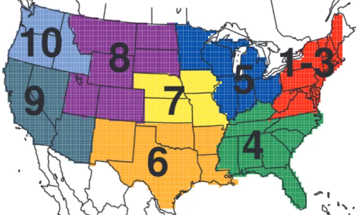
We first simulated present-day levels of ozone and PM2.5 with CMAQ driven by meteorology, chemical boundary con-ditions, anthropogenic emissions, and land-cover that reflect present-day conditions (CURall case). Future ozone and PM2.5 were simulated using CMAQ driven by model inputs that reflect projected conditions for the 2045–2054 (hereafter referred to as future-2050) time period (FUTall case). To ex-amine the individual effects of projected global change pa-rameters on ozone and PM2.5concentrations, four additional attribution cases were simulated. Specifically, these four cases examined the impact of future chemical boundary con-ditions alone (futBC simulation), future anthropogenic emis-sions combined with future land-cover (futEMISfutLU simu-lation), future climate alone (futMETcurLU), and future cli-mate combined with future land-cover (futMETfutLU). All modeling results were grouped and analyzed by EPA region (see Fig. 1). For simplicity, we have combined results from Regions 1, 2, and 3 designated as R1-3.
1-3
4
6
7
5
8
9
10
Fig. 1. EPA regions for the continental United States. Note that
for simplicity Regions 1, 2, and 3 are treated as a single combined region (1-3).
2.1 Model setup
2.1.1 Chemical transport model
The modeling approach is similar to that described in Chen et al. (2008). The CMAQ version 4.4 photochemical grid model was run on a 36-km by 36-km gridded domain, cen-tered over the continental US, with 17 vertical sigma levels from the surface to the tropopause. Gas-phase chemistry was modeled using the SAPRC-99 chemical mechanism (Carter 2000a, b). Aerosol processes were simulated using a modal approach with the AERO3 aerosol module (Byun and Schere, 2006), which includes the ISORROPIA secondary inorganic aerosol algorithms (Nenes et al., 1998) and the SORGAM secondary organic aerosol formulations (Schell et al., 2001). The AERO3 module contains process dynamics for nucle-ation, coagulnucle-ation, condensnucle-ation, evaporation and dry depo-sition (Binkowski et al., 2003). Aerosol species include sul-fates, nitrates, ammonium, primary and secondary organics, and elemental carbon.
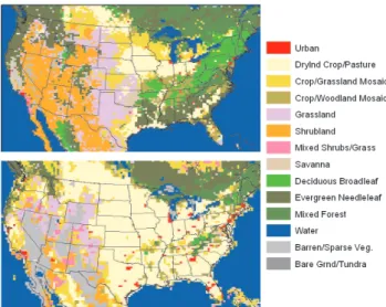
Fig. 2. MM5 land-use by USGS category for the present-day (top)
and future-2050 (bottom) simulations.
2.1.2 Meteorology
To generate the meteorological fields for CMAQ, an MM5-based regional climate model (Salath´e et al., 2008) was used to downscale present-day and future-2050 global climate model results from the NCAR-DOE Parallel Climate Model (PCM, Washington et al., 2000). The PCM model couples at-mospheric, land surface, ocean, and sea-ice modules to form an earth system model for current and future climate scenario projections. The future-2050 PCM simulations were based on the IPCC A2 emission scenario.
The regional climate model is based on the Pennsyl-vania State University (PSU)-National Center for Atmo-spheric Research (NCAR) mesoscale model (MM5) Release 3.6.3 (Grell et al., 1994). Simulations were performed in non-hydrostatic mode with 28 vertical sigma levels, and a one-way nested configuration at 108-km and 36-km grid res-olutions. In order to maintain simulation stability and mass conservation, nudging was employed towards the PCM out-put on the outer 108-km domain. This constrains MM5 to the global model and results in a smooth transition from the global model to the continental scale MM5 simulations.
The MM5 model configurations for the present-day and future-2050 simulations were identical except for the land-use data. Since variations in land-land-use are known to influence regional meteorology and air quality (Civerolo et al., 2000), land-use for the future-2050 simulations was updated with data prepared for the Community Land Model (CLM; Bo-nan et al., 2002), and the Spatially Explicit Regional Growth Model (SERGOM; Theobald, 2005). The SERGOM pro-vided projected urban and suburban population density dis-tributions, while the remaining land-use data was based on a preliminary mapping of plant functional type distributions for the CLM (J. Feddema, personal communications, 2006).
-4 -2 0 2 4 Temperature [C] 400 200 0 -200 -400 PBL [m] -100 -50 0 50 100 -2 -1 0 1 2 0.4 0.2 0.0 -0.2 -0.4 precipitation [cm/day] insolation [watt m-2] water vapor [g/kg] a b c d e
Fig. 3. Projected July changes from the present-day to the 2050’s
for (a) average daily maximum surface temperature, (b) average daily maximum boundary layer height, (c) average daily surface in-solation, (d) average daily water vapor content within the boundary layer, and (e) average daily precipitation.
These maps were based on an interpolation of the Integrated Model to Assess the Global Environment (IMAGEv2.2; Al-camo et al, 1998; Naki´cenovi´c et al., 2000; RIVM, 2002; Strengers et al., 2004). A cross-walk was created to map the CLM land cover plant functional types together with the urban land cover from SERGOM to the MM5 land-use and land-cover categories. Future land-use held natural vegeta-tion constant relative to the present-day land cover dataset, but the natural vegetation was reduced due to simulated agri-culture and grazing represented by the IMAGE 2.2 SRES A2 scenario. Figure 2 depicts the land-use for the present-day and future-2050 simulations. The future land-use maps are dominated by agriculture (shrubs, grasslands and dry-land crops) with large reductions in evergreen forests and wooded wetlands.
Projected changes in average July daily maximum (DM) surface temperature, boundary layer height, downward so-lar radiation, and daily accumulated precipitation, as well as average water vapor content within the boundary layer are shown in Fig. 3. Differences are computed as the 5-year July average in the future simulation minus the present-day sim-ulation. Average DM surface temperatures are projected to increase across the continental US, however, the magnitude of the increase varies greatly by region. The Eastern US is expected to have the largest increase in average DM surface
temperature, with Region 1–3 having a projected increase of +3.4◦C and Region 4 projected to increase by +2.6◦C. The Western US (Region 9) shows comparable changes with Re-gion 4, while the Pacific Northwest (ReRe-gion 10) shows the smallest increase in average DM surface temperature of ap-proximately +1.0◦C. The July average DM PBL height is projected to increase by approximately 100 m or more for most regions, except Regions 6 and 7, which show only slight increases due to offsetting changes in PBL heights within the two regions. In the western half of the US, changes in DM PBL height are directly related to changes in DM surface temperature, where regions with smaller changes in surface temperature (e.g., Texas, California, Oregon) show decreases in PBL heights, and regions with the largest increase in tem-perature (southwestern states) correspond to the largest in-crease in PBL height. In the eastern half of the US, the direct relationship between DM PBL heights and DM sur-face temperature is generally true for the Midwest (excluding parts of Wisconsin) and northeast (excluding parts of New England), while the opposite is true for much of the south-east (excluding most of Florida). In regions where increases in PBL height correspond to increases in temperature, any reduction in air quality due to increased temperatures may be somewhat offset by increases in PBL heights. However, in regions such as the southeast, where reductions in PBL height occur simultaneously with increases in temperature, changes in both meteorological parameters will tend to re-duce air quality. Note that the larger increases in temperature and PBL heights along the coastlines are due to a slight mis-match in the land surface classifications for the present-day and future-2050 scenarios, and are not the result of climate change. The mismatch in land surface classifications does not imply the meteorology is misrepresented in the future-2050 simulations, only that the land-ocean interface has been shifted by one grid cell. The shift has little impact on our overall results because inland grid cells are not affected by whether or not the coast line is one grid cell further away.
The general trend for July surface insolation is a future increase for much of the US due to reduced cloud cover. This implies faster photolysis rates in the atmosphere leading to increased production of photo-reactive pollutants such as ozone. There are, however, regions such as portions of Texas, the Pacific Northwest, and the Southeastern US, which are projected to experience a decrease in surface insolation at the surface due to increased cloud cover, potentially leading to improved air quality in those regions.
Water vapor content is generally projected to increase in the Eastern US, while the Western US shows small regions of slight increases combined with larger areas of decreas-ing water vapor content. Increases in water vapor in rela-tively clean environments (i.e., low NOx) are generally ex-pected to decrease ozone due to the destruction of ozone through photolysis and the removal of the O(1D) molecule via O(1D)+H2O→2OH (Stevenson et al., 2000), as well as through the reaction O3+HO2 →2O2+OH (Racherla and
Adams, 2008). In NOxpolluted environments, increased wa-ter vapor is expected to increase ozone through the compet-ing reaction NO+HO2 → NO2+OH (Racherla and Adams, 2008). The largest changes in precipitation are projected to occur in the southeast, which will increase removal of pollu-tants through wet deposition. Smaller increases in precipita-tion are projected in the northwest and north central regions, while the west central states are generally projected to expe-rience a decrease in precipitation.
2.1.3 Chemical boundary conditions
Both present-day and future-2050 sets of chemical bound-ary conditions were obtained through the downscaling of output from the MOZART-2 (Model for Ozone and Re-lated Chemical Tracers, version 2.4) global chemical trans-port model. The MOZART-2 output used in this work is described by Horowitz (2006). Horowitz (2006) applied MOZART-2 to estimate tropospheric ozone and aerosol con-centrations from 1860 to 2100 based on historical and pro-jected changes in emissions, while the feedbacks from cli-mate change and trends in stratospheric ozone were ig-nored. The historical simulations (1860–1990) were based on the EDGAR-HYDE historical emissions inventory (van Aardenne et al., 1999), while the future simulations (1990– 2100) were based on emissions projections from four dif-ferent IPCC SRES scenarios (A2, A1B, B1, and A1F1). For the purpose of this work, we obtained daily average model results from the IPCC SRES A2 simulations, for July 2000 and July 2050. Note that the meteorological in-puts used to drive the MOZART-2 simulations are not the same as the PCM results used in this work, so some con-sistency is lost. However, the MOZART-2 output does pro-vide a representative set of present-day and projected future-2050 chemical boundary conditions for the CMAQ simula-tions. Generally, for all four boundaries MOZART-2 pre-dicts an increase in ozone of approximately 10 ppbv from the present-day to future-2050 conditions, while NOx and NOy (NO+NO2+HNO3+N2O5+PAN+HNO4+other organic nitrates) increase by approximately 10 pptv and 130 pptv, re-spectively (larger increases, 60 pptv and 230 pptv, were ob-served along the southern boundary). NMVOCs increase ap-proximately 0.7 ppbv, while PM2.5 increased approximately 0.8 µg m−3along the western and southern boundaries, re-flecting projected increases in particulate and precursor emis-sions from Asia and South America. Little to no change in PM2.5is projected along the northern and eastern boundaries. 2.1.4 Regional emissions
The anthropogenic emissions inventory used in this work is based on the 1999 EPA National Emissions Inventory (NEI-1999), and was processed through the SMOKE (Sparse Matrix Operating Kernel Emissions; Houyoux et al., 2005) emissions system. Future anthropogenic emissions were
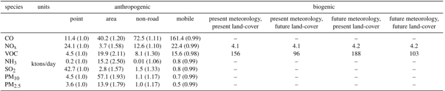
Table 2. Summary of US total present-day and projected future-2050 anthropogenic and biogenic emissions for the month of July. Fractional
change (future-2050 / present-day) is shown in parentheses for anthropogenic emissions.
species units anthropogenic biogenic
point area non-road mobile present meteorology, present meteorology, future meteorology, future meteorology,
present land-cover future land-cover present land-cover future land-cover
CO ktons/day 11.4 (1.0) 40.2 (1.20) 72.5 (1.11) 161.4 (0.99) – – – – NOx 24.1 (1.0) 3.7 (1.58) 12.6 (1.10) 22.4 (0.99) 4.1 4.1 4.2 4.2 VOC 4.5 (1.0) 19.9 (2.11) 8.1 (1.30) 15.6 (0.98) 156 96 188 103 NH3 0.2 (1.0) 15.2 (2.50) 0.01 (1.06) 0.8 (0.99) – – – – SO2 42.7 (1.0) 2.8 (1.57) 1.5 (1.33) 0.8 (0.99) – – – – PM10 4.5 (1.0) 57.1 (1.93) 1.1 (1.17) 0.7 (0.99) – – – – PM2.5 3.6 (1.0) 13.9 (1.79) 1.0 (1.17) 0.5 (0.99) – – – –
projected based on emission growth factors from the EPA Economic Growth Analysis System (EGAS; US EPA, 2004) and extrapolated to 2050 using assumptions consistent with the IPCC A2 scenario. Future emissions accounted for esti-mated population and economic growth, as well as projected energy use by sector. Future emissions did not include re-cent emission control regulations or major technology break-throughs that would affect the use of traditional energy. Fu-ture mobile sources emissions were generated through EGAS based on estimated MOBILE6 VMT growth rates. Mobile emissions estimates considered increases in alternative fuel vehicles and decreases in old vehicle fleets, but the dominant transportation fuels remain gasoline and diesel. The EGAS growth factors were applied to area and mobile source cate-gories, but not to point sources. Future anthropogenic emis-sions were also updated to account for the expansion of urban areas through projected population and housing distributions by the SERGOM model for the year 2030. Present-day and projected future-2050 anthropogenic emissions are summa-rized in Table 2. Area source emissions are projected to expe-rience the largest increase, with emissions for all species, ex-cluding CO, increasing by more than 50%. Non-road emis-sions are projected to increase between 6% and 33%, de-pending on the species, while mobile emissions are projected to remain relatively unchanged.
Biogenic emissions were generated dynamically using MEGAN (Model of Emissions of Gases and Aerosols from Nature; Guenther et al., 2006) with the parameterized form of the canopy environment model. The model estimates hourly isoprene, monoterpene, and other BVOC emissions based on plant functional type and as a function of hourly temperature and ground level shortwave radiation from MM5. Satellite observations of leaf area are used to estimate monthly emis-sion variations associated with leaf age and foliar density. For the current land-cover case, a 1-km seasonal vegetation dataset, derived from satellite and ground observations, was used. For the future-2050 land-cover case, the vegetation dataset was based on the same CLM projected land-cover data used in the MM5 simulations described above (Fig. 2). The CLM land-cover data includes percent coverage of plant functional type and MEGAN includes emission factors based
12000 8000 4000 0 µg-C m-2 hr-1 µg-C m-2 hr-1 12000 8000 4000 0 1600 1200 800 400 0 1600 1200 800 400 0 µg-isoprene m-2 hr-1 µg-isoprene m-2 hr-1
Fig. 4. Biogenic emissions capacity maps (normalized to 30◦C
and 1000 µmoles m−2s−1photosynthetically active radiation) for (a) present-day isoprene, (b) present-day monoterpenes, (c)
future-2050 isoprene, and (d) future-future-2050 monoterpenes.
on plant functional type. For the future-2050 case, MEGAN emission factors were assigned based on the CLM percent cover of plant functional type for a given grid cell.
Projected changes in land-cover resulted in large changes in biogenic emissions capacity from the present-day to future-2050 case (Fig. 4). In the future, isoprene emitting vegetation has been reduced in the south and south eastern states, as well as in the northern mid-west and along the west coast of California. Similarly, a reduction of monoter-pene emitting plants is projected along the west coast of the US and into Southern Canada, as well as in the South and Southeastern US and Eastern Canada. The projected reduc-tion of isoprene and monoterpene emitting plants is suffi-cient to negate any increase in emissions due to increased future temperatures, and results in a net reduction in total future-2050 BVOC emissions compared to the present-day. This work does not include projected changes in biogenic ni-trogen emissions due to increased croplands or changes in management practices in regards to the application of fertil-izers. Table 2 includes a comparison of total continental US biogenic emissions used in the attribution cases: present-day
120 100 80 60 40 20 O3 [ppbv] R01-03 R04 R05 R06 R07 R08 R09 R10 Observed Modeled 98th / 80th / 50th / 20th / 2nd Percentiles
Fig. 5. Comparison of modeled to observed daily maximum 8-h
ozone concentrations.
land-cover with present-day meteorology (CURall and futBC cases), future-2050 land-cover with present-day meteorology (futEMIS case), present-day land-cover with future-2050 meteorology (futMETcurLU case), and future-2050 land-cover with future-2050 meteorology (FUTall and futMET-futLU cases).
3 Results and discussion
In the following sections, we first compare simulated surface ozone and PM2.5 concentrations from the present-day (CU-Rall) simulations to measurements made at monitoring sites throughout the United States. We then analyze and discuss the results of our attribution CMAQ simulations in terms of daily maximum 8-h (DM8H) ozone and average 24-h (A24-h) PM2.5concentrations.
3.1 Ozone and PM2.5evaluation
CMAQ has undergone extensive evaluation for both ozone and PM2.5 model predictions for the continental US (e.g. Eder and Yu, 2006; Phillips and Finkelstein, 2006), and has shown good performance for most regions. CMAQ model evaluations for simulations using downscaled climate model output are limited, but suggest that CMAQ is a suitable tool for use in climate impacts on air quality studies. Hogrefe et al. (2004a) found that CMAQ performed best for predict-ing patterns of average and above average ozone concentra-tions, as well as the frequency distribution of extreme ozone events. Tagaris et al. (2007) found mean 8-h ozone concen-trations were approximately 15% higher than observations, while PM2.5 concentrations were approximately 30% lower than observed. Furthermore, Tagaris et al. (2007) found that PM2.5 model performance is significantly more region spe-cific than mean 8-h ozone performance.
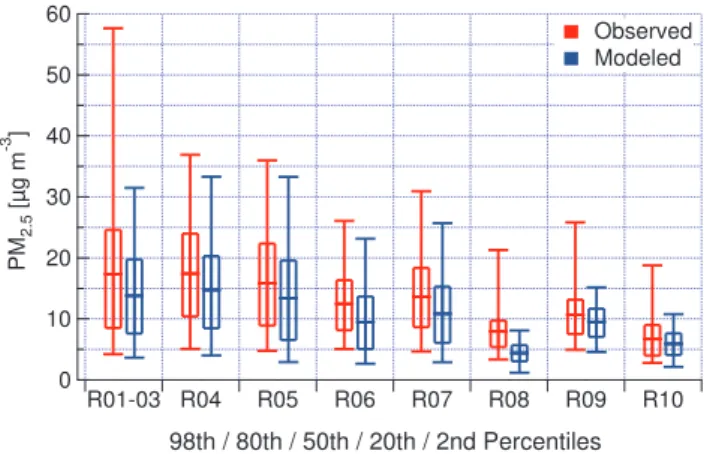
60 50 40 30 20 10 0 PM 2.5 [µg m -3 ] R01-03 R04 R05 R06 R07 R08 R09 R10 Observed Modeled 98th / 80th / 50th / 20th / 2nd Percentiles
Fig. 6. Comparison of modeled to observed average 24-h (A24-h)
PM2.5concentrations.
Model performance is evaluated through a comparison of modeled and observed DM8H ozone and A24-h PM2.5 con-centrations (Figs. 5 and 6). Since our CMAQ simulations were driven by MM5 results that were nudged towards cli-mate model output and not observations, our present-day (CURall) simulations represent a realization of present-day air quality and are not representative of air quality at any specific time (i.e., we cannot do a direct day-to-day or hour-to-hour comparison with observations).
Hourly ozone and daily PM2.5observations were obtained from the EPA AQS database for the five July’s from 1999– 2003. A total of 1349 ozone and 1277 PM2.5monitoring sites were used. Figure 5 compares ranked modeled and observed DM8H ozone concentrations averaged across all sites within each EPA region. Model performance for average DM8H ozone is fairly consistent across all regions, ranging from an over-prediction of +15% in Region 8 to +39% in Region 4. Peak DM8H ozone, represented by the 98th percentile value, shows better performance than the average, and ranges from −2% in Region 9 to +24% in Region 4. Figure 6 compares ranked modeled and observed A24-h PM2.5 concentrations averaged across all sites within each EPA region. Modeled A24-h PM2.5 performance is relatively consistent across all regions, ranging from an under-prediction of −11% in Re-gion 9 to −24% in ReRe-gion 6. The only exception to this is in Region 8, which under-predicts the average by −44%. The peak (98th percentile) 24-h PM2.5concentrations show much more variability compared to the average, and range from under-predictions of −7% to −17% for Regions 4, 5, 6, and 7 to under-predictions of −41% to −62% in Regions 1–3, 8, 9, and 10. These results are consistent with those from our companion paper (Chen et al., 2008) which addressed model performance for ozone for periods extending beyond the July period considered here.
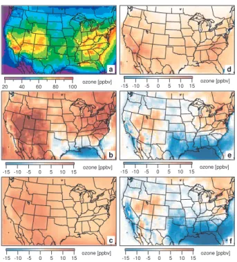
100 80 60 40 20 15 10 5 0 -5 -10 -15 15 10 5 0 -5 -10 -15 15 10 5 0 -5 -10 -15 15 10 5 0 -5 -10 -15 15 10 5 0 -5 -10 -15 ozone [ppbv] ozone [ppbv] ozone [ppbv] ozone [ppbv] ozone [ppbv] ozone [ppbv] a b c d e f
Fig. 7. Average daily maximum 8-h ozone for (a) the CURall
sim-ulation, (b) difference between the FUTall and CURall simulations,
(c) difference between the futBC and CURall simulations, (d)
dif-ference between the futEMIS and CURall simulations, (e) differ-ence between the futMETcurLU and CURall simulations, and (f) difference between the futMETfutLU and CURall simulations.
3.2 Ozone results
The impact of projected future-2050 global changes on sur-face ozone concentrations is spatially highly variable. Some regions experience increases in ozone greater than 10 ppbv (West-Central US), while others see reductions of a few ppbv (Southeastern US). Figure 7 shows a map of the average DM8H ozone concentration for the CURall base case sim-ulation with difference maps for the five attribution simula-tions. Results are summarized by EPA region in Table 3. Fur-ther analysis of the impact of the combined effects of global change upon summertime ozone is given in a companion pa-per by Chen et al. (2008).
On average, projected changes in chemical boundary con-ditions (futBC simulation) have the largest impact on US av-erage DM8H ozone levels (+5 ppbv). The boundary condi-tion impact is more pronounced in the west (+6 ppbv) than in the east (+4 ppbv), due to the predominant westerly flow across the US. As a result, as distance increases from the western boundary, the the boundary conditions have less ef-fect upon ozone levels. These results are consistent with Hogrefe et al. (2004b) who showed that changes in chemi-cal boundary conditions following the IPCC A2 scenario had the largest impact on ozone levels.
Future emissions changes (futEMIS) are projected to in-crease average DM8H ozone levels across the US by an
av-erage of +3 ppbv. The largest increases in avav-erage DM8H ozone are projected to occur in regions that combine in-creases in anthropogenic emissions with sufficient biogenic emissions. In particular, Region 9 in the west and Region 4 in the southeast show the largest increase in average DM8H ozone (+5 ppbv). The smallest increase in average DM8H ozone (+2 ppbv) occurs in Regions 5 and 8, which com-bine relatively smaller increases in anthropogenic emissions with lower future biogenic emissions. Hogrefe et al. (2004b) project a smaller increase in ozone due to future anthro-pogenic emissions with an increase of only 1.3 ppbv in the Eastern US. The discrepancy between Hogrefe et al. (2004b) and the results presented here is most likely due to differ-ences in how future regional anthropogenic emissions are projected. Hogrefe et al. (2004b) projected future US emis-sions based on the IPCC A2 scenario, while emisemis-sions in this work are projected using the EPA EGAS model. In con-trast, Tagaris et al. (2007) found that under the A1b sce-nario a simulated 20% reduction in ozone was primarily due to control-related reductions in emissions within the United States. Similarly, Tao et al. (2007) found that under the IPCC B1 scenario, a projected 4–12% reduction in ozone was dominated by emissions changes, while Steiner et al. (2006) found that projected reductions in California’s anthropogenic emissions had the single largest effect on reducing ozone.
Projected meteorological changes (futMETcurLU simula-tion) result in an overall decrease (−1.3 ppbv) in US average DM8H ozone. Meteorological impacts are spatially highly variable. The largest increases in average DM8H ozone (ap-proximately +4 ppbv), are found in the northeast and west central regions. Our results for the northeast are in agree-ment with Hogrefe et al. (2004b) who found that climate change resulted in an increase of roughly 4 ppbv in aver-age DM8H ozone, as well as, Racherla and Adams (2008) who found that climate change based on the A2 scenario in-creased 95th percentile ozone in the Eastern US by approxi-mately 5 ppbv. In the west central region, increased temper-ature and reduced cloud cover may be somewhat offset by increases in daytime PBL height, but the overall result is an increase in average DM8H ozone. In the northeast, increased average DM8H ozone appears to be due to a combination of increased temperature with only small increases in daytime PBL heights, as well as decreased cloud cover. The largest decreases in average DM8H ozone appear in the south and southwestern regions (−6 ppbv), with smaller decreases oc-curring along the west coast and northern regions (approxi-mately −1 ppbv). The smaller decrease along the west coast is in contrast with Steiner et al. (2006) who found that cli-mate change alone would increase ozone 3-10% throughout California. The large decrease in the south and southeast-ern regions is most likely the result of increased convective precipitation, which enhances the removal of organic nitrates and other reactive nitrogen species, reducing the amount of reactive nitrogen available to participate in ozone chemistry.
Table 3. Average daily maximum 8-h ozone (ppbv) averaged across EPA region for each simulation.
EPA Region CURall FUTall futBC futEMIS futMETcurLU futMETfutLU
R1-3 70 +12 +4 +3 +4 +2 R04 70 +3 +3 +5 −5 −8 R05 63 +7 +4 +2 +1 +0 R06 63 +3 +5 +3 −6 −7 R07 61 +5 +4 +3 −1 −2 R08 62 +9 +6 +2 +0 +0 R09 68 +12 +6 +5 +0 −1 R10 53 +7 +6 +3 −1 −1 US 64 +7 +5 +3 −1.3 −2.6
When projected changes in future land-use are combined with future meteorological conditions (futMETfutLU case), the future average DM8H ozone is spatially very similar to when only meteorological changes are considered (fut-METcurLU case). Accounting for changes in future land-use (i.e., reduced biogenic emissions) has the effect of enhanc-ing the projected decrease in average DM8H ozone. This en-hancement is most pronounced in Region 4, where the largest decreases in BVOC emissions are projected. In Region 4, average DM8H ozone is estimated to decrease an additional 3 ppbv from −5 ppbv to −8 ppbv. On average across the US, the decrease in average DM8H ozone is projected to double from −1.3 ppbv, when climate change alone is considered, to −2.6 ppbv when climate change and future land-use changes are accounted for simultaneously.
The combined effects of projected changes in chemical boundary conditions, emissions, land-use, and climate (FU-Tall simulation) on average DM8H ozone results in the largest increases in the West Central US (e.g., +12 ppbv in Region 9, California) and in the Northeastern US (e.g., +12 ppbv in Region 1–3). In Region 1–3, all of the global changes accounted for in this study lead to increases in av-erage DM8H ozone. The same is true for the eastern por-tion of Region 9. However, in the western porpor-tion of Region 9, changes in chemical boundary conditions and emissions both increase average DM8H ozone, while climate changes have the opposite effect. The largest projected decreases in average DM8H ozone occur in the south and southeast re-gions, where future average DM8H ozone is dominated by climate effects. This is reflected in the relatively small in-creases in average DM8H ozone (+3 ppbv) in Regions 4 and 6. On average across the US, the combined effects of pro-jected global changes result in a +7 ppbv increase in average DM8H ozone, and the changes in ozone are dominated by changes in chemical boundary conditions and emissions in most regions, except for the southeast, which is dominated by changes in convective precipitation.
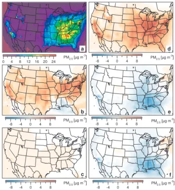
24 20 16 12 8 4 0 -8 -4 0 4 8 -8 -4 0 4 8 -8 -4 0 4 8 -8 -4 0 4 8 -8 -4 0 4 8 PM2.5 [µg m -3 ] PM2.5 [µg m -3 ] PM2.5 [µg m-3] PM2.5 [µg m-3] PM2.5 [µg m -3 ] PM2.5 [µg m-3] a b c d e f
Fig. 8. Average 24-h PM2.5concentration for (a) the CURall
sim-ulation, (b) difference between the FUTall and CURall simulations,
(c) difference between the futBC and CURall simulations, (d)
dif-ference between the futEMIS and CURall simulations, (e) differ-ence between the futMETcurLU and CURall simulations, and (f) difference between the futMETfutLU and CURall simulations.
3.3 PM2.5results
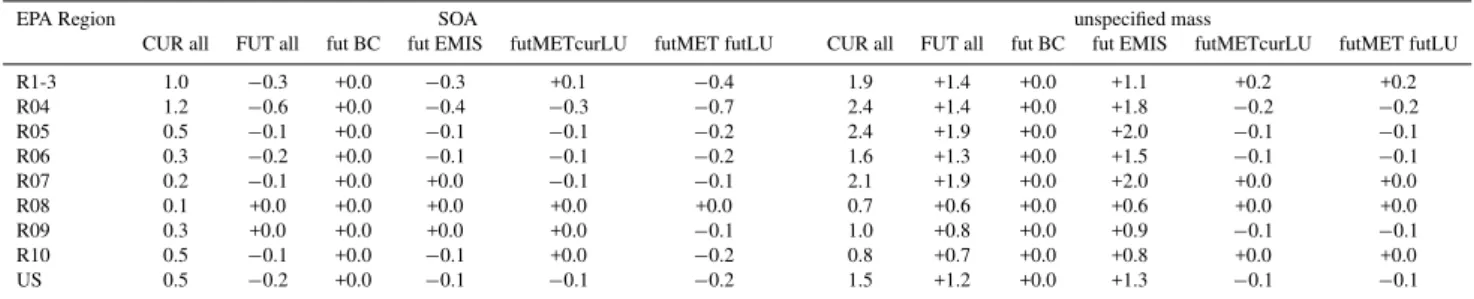
Simulated July A24-h total PM2.5results are shown in Fig. 8 and summarized in Table 4. Results for speciated PM2.5 mass are summarized in Tables 4, 5, 6, and 7. Changes in emissions (futEMIS case) contribute the most to increasing A24-h PM2.5 concentrations across the US (approximately +3 µg m−3). Under the futEMIS case, all speciated PM com-ponents, except for secondary organic aerosol (SOA), con-tribute to increasing PM2.5 mass. SOA is reduced in most
Table 4. Average 24-h concentration (µg m−3) for total PM
2.5 and speciated sulfate (SO4) mass averaged across EPA region for each
simulation.
EPA Region Total PM2.5 SO4
CUR all FUT all fut BC fut EMIS futMETcurLU futMET futLU CUR all FUT all fut BC fut EMIS futMETcurLU futMET futLU
R1-3 11 +4 +0.0 +4 +0.2 +0.4 5.0 +0.9 −0.1 +0.7 +0.0 +0.6 R04 13 +1 +0.3 +5 −3 −3 6.1 −0.6 +0.2 +1.2 −1.8 −1.1 R05 10 +3 +0.2 +5 −1 −1 4.1 −0.1 +0.1 +0.6 −0.8 −0.5 R06 6 +2 +0.4 +3 −1 −1 2.6 +0.0 +0.2 +0.6 −0.7 −0.6 R07 8 +3 +0.3 +4 −1 −1 3.0 +0.0 +0.1 +0.6 −0.7 −0.5 R08 3 +2 +0.3 +1 +0 +0 1.0 +0.4 +0.2 +0.2 +0.0 +0.0 R09 5 +2 +0.6 +2 −0.4 −0.5 1.5 +0.4 +0.3 +0.2 −0.1 −0.1 R10 4 +2 +0.5 +1 −0.2 −0.4 1.2 +0.3 +0.3 +0.1 −0.1 −0.1 US 7 +2 +0.4 +3 −0.9 −0.8 2.9 +0.1 +0.2 +0.5 −0.5 −0.3
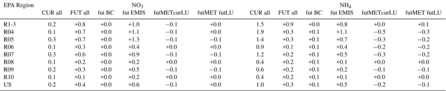
Table 5. Average 24-h concentration (µg ,m−3) for speciated nitrate (NO
3) and ammonium (NH4)mass averaged across EPA region for
each simulation.
EPA Region NO3 NH4
CUR all FUT all fut BC fut EMIS futMETcurLU futMET futLU CUR all FUT all fut BC fut EMIS futMETcurLU futMET futLU
R1-3 0.2 +0.8 +0.0 +1.0 −0.1 +0.0 1.5 +0.9 +0.0 +0.8 +0.0 +0.1 R04 0.1 +0.7 +0.0 +1.1 −0.1 +0.0 1.9 +0.3 +0.1 +1.1 −0.5 −0.3 R05 0.3 +0.7 +0.0 +1.3 −0.1 −0.1 1.4 +0.3 +0.1 +0.7 −0.3 −0.2 R06 0.1 +0.3 +0.0 +0.4 +0.0 +0.0 0.9 +0.1 +0.1 +0.4 −0.2 −0.2 R07 0.3 +0.6 +0.0 +0.9 −0.1 −0.1 1.2 +0.2 +0.1 +0.5 −0.3 −0.2 R08 0.1 +0.2 +0.0 +0.2 +0.0 +0.0 0.4 +0.2 +0.1 +0.1 +0.0 +0.0 R09 0.2 +0.3 +0.0 +0.5 −0.1 −0.1 0.6 +0.2 +0.1 +0.2 −0.1 −0.1 R10 0.1 +0.1 +0.0 +0.2 +0.0 +0.0 0.4 +0.2 +0.1 +0.1 +0.0 +0.0 US 0.2 +0.4 +0.0 +0.6 −0.1 +0.0 1.0 +0.3 +0.1 +0.5 −0.2 −0.1
regions due to decreased biogenic emissions from projected changes in land-cover and from increased production of sul-fate (SO2), nitrate (NO3), and ammonium (NH4)aerosols, which reduces the OH radicals available for SOA production. The largest emissions induced increases in A24-h PM2.5are found in the East and Central US (+4 µg m−3for Regions 1– 3 and 7; +5 µg m−3for Regions 4 and 5), while the smallest changes occur in the west (+1 µg m−3for Regions 8 and 10; +2 µg m−3for Region 9). Unlike ozone, changes in chemical boundary conditions (futBC case) have very little impact on PM2.5 concentrations. A24-h PM2.5 concentrations are in-fluenced most by changes in chemical boundary conditions along the west coast (Regions 9 and 10). For all regions the increase in A24-h PM2.5 is less than +1 µg m−3, with the largest contribution coming from increases in SO4and NH4 mass.
Changes in meteorology (futMETcurLU simulation) result in a slight decrease in A24-h PM2.5 concentrations across the US (approximately −1 µg m−3). The largest decrease in A24-h PM2.5 occurs in Region 4 (−3µg m−3), and is pri-marily due to enhanced precipitation throughout the region and the resulting increase in wet deposition of SO4and NH4. Changes in PM2.5levels across the rest of the US range from +0.2 µg m−3 in Region 1–3 to -1 µg m−3 in Regions 5, 6, and 7. Overall, all speciated PM2.5concentrations either de-cline or remain the same under a future climate, except for
SOA and unspecified PM, which show small increases (0.1-−0.2 µg m−3) in Region 1–3.
Results for the future meteorology and future land-use simulations (futMETfutLU case) show only a slight increase in A24-h PM2.5compared to the future meteorology and cur-rent land-use simulations (futMETcurLU case), which sug-gests that for A24-h PM2.5, meteorological changes are more important than potential changes in future biogenic emis-sions due to land-use changes. The differences in results from the futMETfutLU and futMETcurLU cases are primar-ily due to a decrease in total BVOC emissions (see Fig. 4) and a spatial redistribution of those emissions due to changes in land-cover type (see Fig. 2) in the futMETfutLU case. This decrease in BVOC emissions leads to reduced SOA for-mation and enhanced OH levels, particularly in the east and southeastern regions. The enhanced OH subsequently leads to increases in SO4, NO3, and NH4aerosols compared to the futMETcurLU case. The increase in inorganic aerosol con-centrations offsets the decrease in biogenic SOA, resulting in a small overall increase in A24-h PM2.5 for the futMET-futLU case compared to the futMETcurLU case.
In the FUTall case, A24-h PM2.5 concentration is pro-jected to increase by +2 µg m−3 across the continental US, with the largest increase projected to occur in Region 1–3 (+4 µg m−3). Inorganic PM species SO4, NO3, NH4, and un-specified PM mass contribute the most to increasing A24-h
Table 6. Average 24-h concentration (µg m−3)for speciated elemental carbon (EC) and organic carbon (OC) mass averaged across EPA
region for each simulation.
EPA Region EC OC
CUR all FUT all fut BC fut EMIS futMETcurLU futMET futLU CUR all FUT all fut BC fut EMIS futMETcurLU futMET futLU
R1-3 0.3 +0.1 +0.0 +0.1 +0.0 +0.0 1.0 +0.3 +0.0 +0.2 +0.0 +0.0 R04 0.3 +0.1 +0.0 +0.1 +0.0 +0.0 1.1 +0.1 +0.0 +0.3 −0.2 −0.2 R05 0.3 +0.1 +0.0 +0.1 +0.0 +0.0 0.8 +0.2 +0.0 +0.2 −0.1 −0.1 R06 0.2 +0.0 +0.0 +0.0 +0.0 +0.0 0.6 +0.1 +0.1 +0.2 −0.1 −0.1 R07 0.2 +0.0 +0.0 +0.0 +0.0 +0.0 0.6 +0.1 +0.0 +0.2 −0.1 −0.1 R08 0.2 +0.0 +0.0 +0.0 +0.0 +0.0 0.7 +0.2 +0.0 +0.1 +0.0 +0.0 R09 0.4 +0.1 +0.0 +0.1 +0.0 +0.0 1.4 +0.4 +0.1 +0.3 +0.0 +0.0 R10 0.3 +0.1 +0.0 +0.0 +0.0 +0.0 1.1 +0.4 +0.1 +0.3 +0.0 +0.0 US 0.3 +0.1 +0.0 +0.1 +0.0 +0.0 0.9 +0.2 +0.0 +0.2 −0.1 −0.1
Table 7. Average 24-h concentration (µg m−3)for speciated secondary organic aerosol (SOA) and unspecified mass averaged across EPA
region for each simulation.
EPA Region SOA unspecified mass
CUR all FUT all fut BC fut EMIS futMETcurLU futMET futLU CUR all FUT all fut BC fut EMIS futMETcurLU futMET futLU
R1-3 1.0 −0.3 +0.0 −0.3 +0.1 −0.4 1.9 +1.4 +0.0 +1.1 +0.2 +0.2 R04 1.2 −0.6 +0.0 −0.4 −0.3 −0.7 2.4 +1.4 +0.0 +1.8 −0.2 −0.2 R05 0.5 −0.1 +0.0 −0.1 −0.1 −0.2 2.4 +1.9 +0.0 +2.0 −0.1 −0.1 R06 0.3 −0.2 +0.0 −0.1 −0.1 −0.2 1.6 +1.3 +0.0 +1.5 −0.1 −0.1 R07 0.2 −0.1 +0.0 +0.0 −0.1 −0.1 2.1 +1.9 +0.0 +2.0 +0.0 +0.0 R08 0.1 +0.0 +0.0 +0.0 +0.0 +0.0 0.7 +0.6 +0.0 +0.6 +0.0 +0.0 R09 0.3 +0.0 +0.0 +0.0 +0.0 −0.1 1.0 +0.8 +0.0 +0.9 −0.1 −0.1 R10 0.5 −0.1 +0.0 −0.1 +0.0 −0.2 0.8 +0.7 +0.0 +0.8 +0.0 +0.0 US 0.5 −0.2 +0.0 −0.1 −0.1 −0.2 1.5 +1.2 +0.0 +1.3 −0.1 −0.1
PM2.5 both in Region 1–3 and for the US as a whole, while changes in SOA tend to reduce PM levels in all regions. The smallest increase in A24-h PM2.5 is projected to occur in Region 4 (+1 µg m−3), where reductions in SOA are largest and increased precipitation leads to enhanced removal of PM through wet deposition.
4 Conclusions
Changes in future ozone and PM2.5 concentrations com-pared to the present-day, are due to the synergistic effects of changes in chemical boundary conditions, regional an-thropogenic emissions, land-use/land-cover (biogenic emis-sions), and climate. We have presented a comprehensive ap-proach to addressing the individual and combined effects of these global changes on future US air quality through the off-line coupling of global and regional climate, chemical trans-port, and emissions models. Although other work has ad-dressed the impact of various global changes on air quality, to our knowledge, this is the first study to address a number of these global changes in such a comprehensive manner.
Overall, US July average DM8H ozone concentrations in the 2050’s are projected to increase by an average of +7 ppbv compared to the present-day. However, these results are spa-tially highly variable. Some regions may experience larger increases in average DM8H ozone, while other regions may
experience decreases in average DM8H ozone. Projected changes in chemical boundary conditions are found to have the single largest impact on average DM8H ozone, and in-crease ozone levels in all regions. The second largest impact on ozone levels is due to changes in anthropogenic emissions combined with future land-use (i.e., reduced BVOC emis-sions), which increase ozone in most regions, except in large urban centers, where ozone decreases. Climate change alone is projected to increase average DM8H ozone in some re-gions (northeast and west central), and decrease it in oth-ers (west coast and south/southeast), but results in an overall decrease of ozone. When projected changes in climate and land-use are simultaneously accounted for, average DM8H ozone is decreased even further.
Projected increases in future A24-h PM2.5 concentra-tions are primarily driven by increases in inorganic aerosol concentrations, which more than offset any decreases in biogenic SOA associated with the reduced BVOC emis-sions (from projected land-use changes). Projected changes in chemical boundary conditions result in a negligible in-crease (<1 µg m−3) in A24-h PM2.5concentrations. Climate change tends to reduce PM2.5concentrations in most regions, with the largest reductions coming in the Southeastern US due to enhanced wet deposition from an increase in convec-tive precipitation.
The results from this work show that although climate change may play an important role in defining future air qual-ity in certain regions, on a larger scale, changes in chemical boundary conditions and emissions appear to play a much more important role. This is consistent with recent work by Tao et al. (2007) who show that the importance of specific global changes to projected air quality will change depend-ing on which future climate/emissions scenario is assumed. Furthermore, the variability in the results from recent mod-eling studies examining the impact of global changes on US air quality (e.g. Wu et al., 2008; Racherla and Adams, 2008; Tagaris et al., 2007; Dentener et al., 2006; Murazaki and Hess, 2006) illustrates the difficulty involved in making these predictions, as well as the necessity for including all avail-able studies when evaluating the potential impacts of global changes on future US air quality. The results presented here are representative of summertime climatology only, where the summertime is represented by five present-day or future July’s. Although five July’s are fairly representative of the middle of the ozone season, elevated PM2.5 can occur year-round, and the climatological and emissions drivers that im-pact PM2.5in the summertime may be very different at other times of the year. To examine the relationship between spe-cific global changes and regional air quality more thoroughly, we plan to conduct a matrix of additional model runs cover-ing both summer and winter months, that will include multi-ple future climate, global/regional anthropogenic emissions, and land-use/land-cover scenarios.
Acknowledgements. The authors would like to thank Dr. Larry
Horowitz (NOAA Geophysical Fluid Dynamics Laboratory) for providing the global MOZART-2 output, Dr. David Theobald (Colorado State University) for providing projected urban and suburban population density distributions, Dr. Lawrence Buja and Gary Strand (National Center for Atmospheric Research) for providing the PCM output, and Dr. Johannes Feddema (University of Kansas) for providing the future land-cover dataset. This work was supported by the EPA Science to Achieve Results (STAR) Pro-gram (Agreement Number: RD-83096201). EPA has not officially endorsed this publication and the views expressed herein may not reflect the views of the EPA. This publication is partially funded by the Joint Institute for the Study of the Atmosphere and Ocean (JISAO) under NOAA Cooperative Agreement No. NA17RJ1232, Contribution #1583. This research uses data provided by the Parallel Climate Model project www.cgd.ucar.edu/pcm), supported by the Office of Biological and Environmental Research of the US Department of Energy and the Directorate for Geosciences of the National Science Foundation.
Edited by: F. J. Dentener
References
Alcamo, J., Leemans, R., and Kreileman, E.: Global change sce-narios of the 21st century. Results from the IMAGE 2.1 model. Pergamon & Elseviers Science, London, UK, 296 pp., 1998. Binkowski F. S. and Roselle, S. J.: Models-3 Community
Multiscale Air Quality (CMAQ) model aerosol component 1. Model description, J. Geophys. Res., 108(D6), 4183, doi:10.1029/2001JD001409, 2003.
Bonan, G. B., Oleson, K. W., Vertenstein, M., Levis, S., Zeng, X. B., Dai, Y. J., Dickinson, R. E., and Yang, Z. L.: The Land Sur-face Climatology of the Community Land Model Coupled to the NCAR Community Climate Model, J. Climate, 15(22), 3123– 3149, 2002.
Byun, D. and Schere, K. L.: Review of the Governing Equa-tions, Computational Algorithms, and Other Components of the Models-3 Community Multiscale Air Quality (CMAQ) Model-ing System, Appl. Mech. Rev., 59, 51–77, 2006.
Carter, W.: Documentation of the SAPRC-99 Chemical Mecha-nism for VOC Reactivity Assessment, Draft report to the Cal-ifornia Air Resources Board, Contracts 92–329 and 95–308, 8 May 2000a.
Carter, W.: Implementation of the SAPRC-99 Chemical Mecha-nism into the Models-3 Framework, Report to the United States Environmental Protection Agency, 29 January 2000b.
Chen, J., Avise, J., Lamb, B., Salathe, E., Mass, C., Guenther, A., Wiedinmyer, C., Lamarque, J.-F., O’Neill, S., McKenzie, D., and Larkin, N.: The effects of global changes upon regional ozone pollution in the United States, Atmos. Chem. Phys., submitted, 2008.
Civerolo, K. L., Sistla, G., Rao, S. T., and Nowak, D. J.: The Ef-fects of Land Use in Meteorological Modeling: Implications for Assessment of Future Air Quality Scenarios, Atmos. Environ., 34(10), 1615–1621, 2000.
Constable, J., Guenther, A., Schimel, D., and Monson, R.: Model-ing changes in VOC emission in response to climate change in the continental United States, Glob. Chang. Biol., 5, 791–806, 1999.
Dawson, J. P., Adams, P. J., and Pandis, S. N.: Sensitivity of ozone to summertime climate in the eastern USA: A modeling case study, Atmos. Environ., 41, 1494–1511, 2007.
Dentener, F., Stevenson, D., Ellingsen, K., et al.: The Global At-mospheric Environment for the Next Generation, Environ. Sci. Technol., 40, 3586–3594, 2006.
Eder, B. and Yu, S.: A performance evaluation of the 2004 release of Models-3 CMAQ, Atmos. Environ., 40, 4811–4824, 2006. Grell, G. A., Dudhia, J., and Stauffer, D. R.: A Description of the
Fifth-Generation Penn State/NCAR Mesoscale Model (MM5), National Center for Atmospheric Research, Boulder, CO, USA, NCAR/TN-398+STR, 122 pp., 1994.
Guenther, A., Karl, T., Harley, P., Wiedinmyer, C., Palmer, P. I., and Geron, C.: Estimates of global terrestrial isoprene emissions using MEGAN (Model of Emissions of Gases and Aerosols from Nature), Atmos. Chem. Phys., 6, 3181–3210, 2006,
http://www.atmos-chem-phys.net/6/3181/2006/.
Heald, C. L., Henze, D. K., Horowitz, L. W., Feddema, J., Lamar-que., J.-F., Guenther, A., Hess, P. G., Vitt, F., Seinfield, J. H., Goldstein, A. H., Fung, I.: Predicted change in global sec-ondary organic aerosol concentrations in response to future cli-mate, emissions, and land use change, J. Geophys. Res., 113,
D05211, doi:10.1029/2007JD009092, 2008.
Hogrefe, C., Biswas, J., Lynn, B., Civerolo, K., Ku, J.-Y., Rosen-thal, J. Rosenzweig, C., Goldberg, R., and Kinney, P. L.: Simu-lating regional-scale ozone climatology over the eastern United States: model evaluation results, Atmos. Environ., 38, 2627– 2638, 2004a.
Hogrefe, C., Lynn, B., Civerolo, K., Ku, J.-Y., Rosenthal, J., Rosenzweit C., Goldberg R., Gaffin, S., Knowlton, K., and Kinney, P. L.: Simulating changes in regional air pollution over the eastern United States due to changes in global and re-gional climate and emissions, J. Geophys. Res., 109, D22301, doi:10.1029/2004JD004690, 2004b.
Horowitz, L. W.: Past, present, and future concentrations of tro-pospheric ozone and aerosols: Methodology, ozone evaluation, and sensitivity to aerosol wet removal, J. Geophys. Res., 111, D22211, doi:10.1029/2005JD006937, 2006.
Houyoux, M., Vukovich, J., and Brandmeyer, J. E.: Sparse Ma-trix Operator Kernel Emissions (SMOKE) modeling system user manual, University of North Carolina at Chapel Hill, online available at: http://www.smoke-model.org, last access: 2009, 2005.
Jaffe, D. A., Parish, D., Goldstein, A., Price, H., and Harris, J.: Increasing background ozone during spring on the west coast of North America, Geophys. Res. Lett., 30(12), 1613, doi:10.1029/2003GL017024, 2003.
Leung, L. R. and Gustafson Jr., W. I.: Potential regional climate and implications to US air quality, Geophys. Res. Lett., 32, L16711, doi:10.1029/2005GL022911, 2005.
Liao, K.-J., Tagaris, E., Manomaiphiboon, K., Wang, C., Woo, J.-H., Amar, P., He, S., and Russell, A. G.: Quantification of the im-pact of climate uncertainty on regional air quality, Atmos. Chem. Phys., 9, 865–878, 2009,
http://www.atmos-chem-phys.net/9/865/2009/.
Marenco, A., Gouget, H., N´ed´elec, P., Pag´es, J.-P., and Karcher, F.: Evidence of a long term increase in tropospheric ozone from Pic du Midi data series: Consequences: positive radiative forcing, J. Geophys. Res., 99, 16617–16632, 1994.
Mickley, L. J., Jacob, D. J., and Field, B. D.: Effects of future climate change on regional air pollution episodes in the United States, Geophys. Res. Lett., 31, L24103, doi:10.1029/2004GL021216, 2004.
Murazaki, K. and Hess, P.: How does climate change contribute to surface ozone change over the United States?, J. Geophys Res., 111, D05301, doi:10.1029/2005JD005873, 2006.
Naki´cenovi´c, N., Alcamo, J., Davis, G., de Vries B., Fenhann, B., Gaffin, S., Gregory K., Gr¨ubler, A., Jung, T. Y., Kram, T., La Rovere, E. L., Michaelis, E. L., Mori, S., Morita, T., Pepper, W., Pitcher, H., Price, L., Raihi, K., Roehrl, A., Rogner, H.-H., Sankovski, A., Schlesinger, M., Shukla, P., Smith, S., Swart, R., van Rooijen, S., Victor, N., and Dadi, Z.: IPCC Special Report on Emissions Scenarios, Cambridge University Press, Cambridge, UK and New York, NY, USA, 2000.
Nenes, A., Pandis, S. N., and Pilinis, C.: ISORROPIA: A new ther-modynamic equilibrium model for multiphase multicomponent inorganic aerosols, Aquat. Geochem., 4, 123–152, 1998. Phillips, S. B. and Finkelstein, P. L.: Comparison of spatial patterns
of pollutant distribution with CMAQ predictions, Atmos. Envi-ron., 40, 4999–5009, 2006.
Racherla, P. N. and Adams, P. J.: The response of surface ozone
to climate change over the Eastern United States, Atmos. Chem. Phys., 8, 871–885, 2008,
http://www.atmos-chem-phys.net/8/871/2008/.
RIVM (Rijks Instituut voor Volksgezondheid en Milieu): IMAGE 2.2 CD release and documentation. The IMAGE 2.2 implemen-tation of the SRES scenarios: A comprehensive analysis of emis-sions, climate change and impacts in the 21st century, for further information online available at: http://www.rivm.nl/image/index. html, 2002.
Salath´e, E. P., Steed, R., Mass, C. F., and Zahn, P.: A high-resolution climate model for the United States pacific northwest: Mesoscale feedbacks and local responses to climate change, J. Climate, in press, 2008.
Schell, B., Ackermann, I., Hass, H., Binkowski, F., and Ebel, A.: Modeling the formation of secondary organic aerosol within a comprehensive air quality model system, J. Geophys. Res., 106(D22), 28275–28293, 2001.
Sillman S. and Samson, P. J.: Impact of temperature on oxidant pho-tochemistry in urban, polluted rural, and remote environments, J. Geophys. Res., 100, 11497-11508, 1995.
Staehelin, J., Thudium, J., Buehler, R., Volz-Thomas, A., and Graber, W.: Trends in Surface Ozone Concentrations at Arosa (Switzerland), Atmos. Environ., 28, 75–87, 1994.
Steiner, A. L., Tonse, S., Cohen, R. C., Goldstein, A. H., and Harley, R. A.: Influence of future climate and emissions on regional air quality in California, USA, J. Geophys. Res., 111, D18303, doi:10.1029/2005JD006935, 2006.
Stevenson, D. S., Johnson, C. E., Collins, W. J., Derwent, R. G., and Edwards, J. M.: Future estimates of tropospheric ozone radiative forcing and methane turnover - the impact of climate change, Geophys. Res. Lett., 105(14), 2073–2076, doi:10.1029/1999GL010887, 2000.
Strengers, B., Leemans, R., Eickhout, B., de Vries, B., and Bouw-man, L.: The land-use projections and resulting emissions in the IPCC SRES scenarios as simulated by the IMAGE 2.2 model, GeoJournal, 61, 381–393, 2004.
Tagaris, E., Manomaiphiboon, K., Liao, K.-J., Leung, L. R., Woo, J.-H., He, S., Amar, P., and Russel, A. G.: Impacts of global cli-mate change and emissions on regional ozone and fine particulate matter concentrations over the United States, J. Geophys. Res., 112, D14312, doi:10.1029/2006JD008262, 2007.
Tao, Z., Williams, A., Huang, H.-C., Caughey, M., and Liang, X.-Z.: Sensitivity of US surface ozone to future emis-sions and climate changes, Geophys. Res. Lett., 34, L08811, doi:10.1029/2007GL029455, 2007.
Theobald, D. M.: Landscape Patterns of Exurban Growth in the USA From 1980 to 2020, Ecol. Soc., 10(1), p. 32, 2005. US EPA: Economic Growth Analysis System (EGAS) version 5.0
User Manual, US Environmental Protection Agency, 2004. van Aardenne, J. A., Carmichael, G. R., Levy II, H., Streets, D., and
Hordijk, L.: Anthropogenic NOx emissions in Asia in the period 1990-2020. Atmos. Environ., 33, 633–646, 1999.
Varotsos, C. and Cartalis, C.: Re-evaluation of surface ozone over Athens, Greece, for the period 1901–1940, Atmos. Res., 26, 303–310, 1991.
Vingarzan, R. and Thomson, B.: Temporal variation in daily con-centrations of ozone and acid related substances at Saturna Is-land, British Columbia, J. Air Waste Manage. Assoc., 54, 459– 472, 2004.
Washington, W. M., Weatherly, J. W., Meehl, G. A., Semtner, A. J., Bettge, T. W., Craig, A. P., Strand, W. G., Arblaster, J., Wayland, V. B., James, R., and Zhang, Y.: Parallel Climate Model (PCM) control and transient simulations. Climate Dyn., 16(10–11), 755– 774, 2000.
Wiedinmyer, C., Tie, X., Guenther, A., Neilson, R., and Granier, C.: Future changes in biogenic isoprene emissions: how might they affect regional and global atmospheric chemistry?, Earth Int., 10(3), 1–19, 2006.
Wu, S., Mickley, L. J., Leibensperger, E. M., Jacob, D. J., Rind, D., and Streets, D. G.: Effects of 2000–2050 global change on ozone air quality in the United States, J. Geophys. Res., 113, D06302, doi:10.1029/2007JD008917, 2008.