Performance of podded propulsors in opens tests

(1)

Publisher’s version / Version de l'éditeur:

Vous avez des questions? Nous pouvons vous aider. Pour communiquer directement avec un auteur, consultez la première page de la revue dans laquelle son article a été publié afin de trouver ses coordonnées. Si vous n’arrivez Questions? Contact the NRC Publications Archive team at

[email protected]. If you wish to email the authors directly, please see the first page of the publication for their contact information.

https://publications-cnrc.canada.ca/fra/droits

L’accès à ce site Web et l’utilisation de son contenu sont assujettis aux conditions présentées dans le site LISEZ CES CONDITIONS ATTENTIVEMENT AVANT D’UTILISER CE SITE WEB.

Student Report (National Research Council of Canada. Institute for Ocean Technology); no. SR-2007-05, 2007

READ THESE TERMS AND CONDITIONS CAREFULLY BEFORE USING THIS WEBSITE. https://nrc-publications.canada.ca/eng/copyright

NRC Publications Archive Record / Notice des Archives des publications du CNRC :

https://nrc-publications.canada.ca/eng/view/object/?id=e927e06e-fe53-4bc6-82b2-c1a97fa658af https://publications-cnrc.canada.ca/fra/voir/objet/?id=e927e06e-fe53-4bc6-82b2-c1a97fa658af

For the publisher’s version, please access the DOI link below./ Pour consulter la version de l’éditeur, utilisez le lien DOI ci-dessous.

https://doi.org/10.4224/8895869

Access and use of this website and the material on it are subject to the Terms and Conditions set forth at

Performance of podded propulsors in opens tests Rossiter, C.

(2)

DOCUMENTATION PAGE

REPORT NUMBER

SR-2007-05

NRC REPORT NUMBER DATE

April 2007

REPORT SECURITY CLASSIFICATION DISTRIBUTION

TITLE

Performance of Podded Propulsors in Opens Test

AUTHOR(S)

C. Rossiter

CORPORATE AUTHOR(S)/PERFORMING AGENCY(S)

Institute for Ocean Technology, National Research Council, St. John’s, NL PUBLICATION

SPONSORING AGENCY(S)

IMD PROJECT NUMBER NRC FILE NUMBER

KEY WORDS

Podded Propulsor, AziPod, Props, Propulsion, Propeller

PAGES FIGS. TABLES

SUMMARY

This report describes the experiments carried out here at IOT in March of 2007 on the NRC-IOT Podded Propulsor model, which is a scaled model of the MUN-NSERC with a scale factor of 1:1.35. It also compares these experiments with two other cases. These cases consist of the tests conducted at MUN on the MUN-NRC-NSERC model in January of 2005 and a simulation of these tests done with PROPELLA.

With these new tests, the data suggests that the definition of the performance envelop of podded propulsors should be increased. Further testing plans include the building of a model vessel where model self-propulsion tests will be conducted.

ADDRESS National Research Council Institute for Ocean Technology Arctic Avenue, P. O. Box 12093 St. John's, NL A1B 3T5

(3)

National Research Council Conseil national de recherches

Canada Canada

Institute for Ocean Institut des technologies

Technology océaniques

Performance of Podded Propulsors in Opens Test

SR-2007-05

Christopher P. A. Rossiter

(4)

List of Tables

Table 1: Geometric particulars of NRC-IOT model podded propulsor... 4

Table 2: Geometric particulars of MUN-NRC-NSERC model ... 5

Table 3: Weights used in thrust and torque calibrations... 14

Table 4: General test plan for Air Friction Tests, Case 1 ... 20

Table 5: General test plan for Bollard Runs, Case 1... 20

Table 6: General test plan for Opens Tests, Case 1 ... 20

Table 7: General test plan for Air Friction Tests, Case 3 ... 21

Table 8: General test plan for Bollard Runs, Case 3... 21

(6)

List of Figures

Figure 1: A Podded Propulsor... 1

Figure 2: Towing tank facility at IOT – plan view ... 3

Figure 3: A cross section of the towing tank at IOT... 3

Figure 4: A schematic of the IOT (and MUN-NRC-NSERC) model... 5

Figure 5: Fully instrumented IOT podded propulsor model... 6

Figure 6: The MUN-NRC-NSERC pod model... 8

Figure 7: Model stern for IOT pod model tests ... 9

Figure 8: DAS Set-up used for calibrations... 10

Figure 9: Thrust Torque Calibration Set-Up (In Tension)... 12

Figure 10: Thrust Torque Calibration Set-Up, (Torque Applied)... 13

Figure 11: Experimental Set-Up in Towing Tank ... 15

Figure 12: Experimental Set-Up in Towing Tank (2)... 16

Figure 13: Typical Static Run Sequence Showing Segments... 18

Figure 14: Typical Dynamic Run Sequence Showing Segments ... 19

Figure 15: Comparison of Kt, 10Kq, and KFx ... 22

Figure 16: Comparison of KFx, KFy, KFz ... 23

Figure 17: Kt, 10Kq, KFx for NRC-IOT Tests... 24

Figure 18: KFx, KFy, KFz for NRC-IOT Tests... 24

Figure 19: Kt, 10Kq, KFx vs Azimuthing Angle, at J=0.4... 25

(7)

List of Appendices

Appendix A: Calibration Data

Appendix B: Run Log

(8)

List of Abbreviations

IOT Institute for Ocean technology

TC Transport Canada

CMS Centers for Marine Simulation

OERC Ocean Engineering Research

MUN Memorial University of Newfoundland

NRC National Research Council

m Metre ft Feet kg Kilograms kW Kilowatts kHz Kilohertz P/D Pitch-Diameter Ratio

EAR Expanded Area Ratio

D Diameter

L Length

Mm Millimeters

Deg Degrees

NSERC Natural Sciences and Engineering Research Council of Canada

T Thrust

Q Torque

V Carriage Speed

n Rotational Speed of the Propeller

DAS Data Acquisition System

in Inches

N Newton

N-m Newton-meters

RPS Revolutions Per Second

F Force

(9)

1.0 Introduction

This report describes some of the experiments conducted under the Podded Propulsion project - a collaborative project between Institute for Ocean Technology (IOT), Transport Canada (TC), Centers for Marine Simulation (CMS) and Ocean Engineering Research (OERC) at the Memorial University of Newfoundland (MUN). Transport Canada is a department within the government ,which is responsible for developing regulations, policies and services of transportation in Canada. Transport Canada has regulations, standards and programs to oversee the safety, security and marine infrastructure for operators and passengers of small vessels, large commercial vessels and pleasure craft. Transport Canada also has rules to govern the safe transport of dangerous goods by water, and to protect the marine environment. Transport Canada is committed to working with industry stakeholders and the public to strengthen and encourage compliance with regulations and safe marine practices.

Azimuthing Podded Propulsors were introduced to the marine industry over a decade ago and now are a popular main propulsion system for ships. The Queen Mary II is equipped with four Rolls Royce Mermaid podded propulsion units. A podded propeller consists of a motor inside a pod and a propeller connected to a drive shaft. The propellers are

connected to one or both ends of the drive shaft. The unit is connected to the vessel via a strut, which allows the system to rotate through 360° around the vertical axis (azimuth), making for rapid changes in thrust direction and eliminating the need for a conventional rudder.

The purpose of the project is to develop a suit of simulation tools capable of simulating vessels driven by podded propulsors and implementing them in to the simulator at the CMS. The purpose of the experiments described in this report is to generate the

knowledge base to develop the mathematical algorithms suitable for CMS simulator. The algorithms will predict the performance of a single podded propulsor in different

operational scenarios. The data collected from this report while be utilized by Transport Canada to update their regulations.

Figure 1: A Podded Propulsor

(10)

2.0 Description of Facilities

This section describes the facilities used during the experiments.

2.1 Description of NRC-IOT Towing Tank

IOT’s Towing Tank is a rectangular tank 200m (656 ft) in length, 12m (39 ft) in width and 7m (23 ft) in depth, models are towed through still water or waves by a carriage spanning the width of the tank, model rigging is facilitated by two trim docks and a moveable overhead crane.

The Towing Tank is also equipped with a single manned carriage with 8 wheel

synchronous motor drive and test frame adjustable for model size. The carriage weighs 80000 kg, has 746 kW power, speed ranges from .001 m/s - 10.0 m/s, and manual service carriage for wind and current generation.

It’s Wave Generator consists of a dual flap hydraulic wave board with digital computer control, regular or irregular waves program controlled, and a maximum regular wave height of 1m or 0.5m significant. The Wave Absorber is a parabolic corrugated surface beach with transverse slats, 20m long with 10.5-degree slope at water line, flexible side absorbers. It’s wind generator is capable of reaching wind speeds up to 12m/s and 10m from fans.

The model size ranges for the tank are ship models up to 12m in length and floating structures 0.5m - 4m in diameter.

Its instrumentation consists of force measurement, strain gauge load cells, capacitance and sonic wave probes, model position, QUAIISYS optical tracking, accelerometer arrays and motions package for model motions, propeller characteristics, open water propeller dynamometer, propulsion and control system for free-running models, under and above water video, transient recorders, and flow measurement. Its Data Acquisition System consists of a VMS and Windows NT based distributed client/server system using one or more IOtech DaqBoards, each with 256 channel capability at 100kHz aggregate. 1

(11)

Figure 2: Towing tank facility at IOT – plan view

(12)

3.0 Description of Models

This section describes the models used for the experiments in MUN Towing Tank and the experiments NRC in the NRC-IOT Towing Tank. The dimension for each model can be found in Figure 5.

3.1 Description of NRC-IOT Physical Model

The tests described in this report were conducted using a single podded propulsor in the towing tank facility at IOT. The model was scaled version of the MUN-NRC-NSERC model (with a scale factor of 1:1.35). The propeller was a left-handed propeller. It had four blades, a pitch-diameter ratio (P/D) of 1.0, and an expanded area ratio (EAR) of 0.6. The model propulsor was designated as Pod A as later experiments were planned using twin pods. The arrangement is given in Description of Tests section of this report. The design of the geometry of the podded propulsor was done in a previous and provided an average representation of a full scale single screw podded propellers available in

literature. The geometric particulars of the model are given below in Table 1.

Table 1: Geometric particulars of NRC-IOT model podded propulsor

Experimental Dimensions of Model Podded Propulsors

Pod Measurements

Propeller Diameter, DProp 200

Pod Diameter, DPod 102.96

Pod Length, LPod 303.7

Strut Height, SHeight 222.22

Strut Chord Length 166.67

Strut Distance, SDist 74.07

Strut Width 44.44

Fore Taper Length 62.96

Fore Taper Angle 11.11

Aft Taper Length 81.48

Aft Taper Angle 18.52

(13)

Figure 4: A schematic of the IOT (and MUN-NRC-NSERC) model

3.2 Description of the MUN-NRC-NSERC Pod Model

In this report, comparisons were provided with earlier experiments conducted using MUN-NRC-NSERC Pod Model – done at the towing tank facility of MUN. The model is a scaled up version of the IOT model descried above (scale 1: 1.35). The diameter of its propeller is 270mm. Some of the geometric particulars of the MUN-NRC-NSERC Pod Model are given below in Table 2 and Figure 4.

Table 2: Geometric particulars of MUN-NRC-NSERC model

Experimental Dimensions of Model Podded Propulsors

Pod Measurements

Propeller Diameter, DProp 270 mm

Pod Diameter, DPod 139 mm

Pod Length, LPod 410 mm

Strut Height, SHeight 300 mm

Strut Chord Length 225 mm

Strut Distance, SDist 100 mm

Strut Width 60 mm

Fore Taper Length 85 mm

Fore Taper Angle 15 deg

Aft Taper Length 110 mm

(14)

4.0 Description of Instrumentation

The following section describes the instrumentation used at both test facilities.

4.1 NRC-IOT Dynamometer

The set-up shown below in Figure 5 was used for this set of experiments. The system has the ability to measure the propeller and pod forces and moments. It measures unit thrust (Tunit) propeller thrust at the propeller hub (Tprop), propeller torque (Q), as well as forces in the three coordinate directions.The unit thrust is of particular interest, as it is used for powering predictions for podded propellers. The unit thrust is the net available thrust available for propelling the ship. It not only includes the thrust of the propeller, but also the drag and other hydrodynamic forces acting on the pod-strut body.

The design includes an instrumented propeller hub, a custom mitre gearbox, an azimuth drive system, a propeller drive system, a hull mounting and seal assembly, and a six-component balance for measuring global loads on the pod. 4

(15)

4.2 The MUN-NRC-NSERC Pod Dynamometer

The custom designed MUN-NRC-NSERC pod dynamometer system, was used during the previous experiments, of which the results were used to compare to the present IOT model tests The system has the ability to measure the propeller and pods forces and moments. It is capable of measuring unit thrust (Tunit), propeller thrust at the hub end (Tprop), propeller thrust at the pod end (Tpod), propeller torque (Q), as well as forces in the three coordinate directions. 2The unit thrust is of particular interest, as it used for

powering predictions for podded propellers.. The water temperature, carriage speed (V), and the rotational speed of the propeller (n) were also measured during the experiments. As can be seen above in Figure 5, the unit consists of two major components. The first part is the pod dynamometer, which measures the thrust and torque of the propeller at the propeller shaft. The second part of the unit is the global dynamometer, which measures the unit forces in the three coordinate directions at a location above the propeller boat. Also, a boat shaped body called a wave shroud was attached to the frame of the test equipment and placed just above the water surface. Further details of the experimental apparatus can be found in MacNeill et al. (2004). 5

(16)

Figure 6: The MUN-NRC-NSERC pod model

(17)

4.3 Model Stern

For the tests done in the NRC-IOT Towing Tank with the IOT pod model a model stern with holes in the floor was used to hold the test equipment. The pod drives fit through the holes and the dynamometer rested on the model stern. The distance between the drives could be varied. The model stern also has a plexiglas floor so any disturbance at the water’s surface can be seen during the test runs.

(18)

4.4 Data Acquisition System (DAS) for IOT Pod Model Tests

The Data Acquisition System for this project is custom built with IOTech gear and RS232 data from the U500 controller. The system components were chosen to allow for the system to be placed into a free running model. The data was collected through a total of 26 channels. The system consisted of the following:

- 1 - Panasonic CF-51 Laptop, PC4026, S/N - 1 – Panasonic Docking Station

- 1 – D-Link DI-624 Wireless Router - 1 - IOTech Daqbook 2001, S/N 802671

- 2 - IOTech DBK 43A, 8 Channel Stain Gage Modules - 1 – Custom 16 Channel DBK 43A to 10 Pin breakout box - 2 - IOTech DBK 45, 4-Channel SSH and Low-Pass Filter Cards - 1 – IOTech DBK 10, Expansion Chassis

- 1 – Custom 8-Channel Isolation Amp box

(19)

5.0 Calibrations

The method used to calibrate the global dynamometer as well as thrust and torque load cells was the linear least squares method. This method theorizes that if enough varied loads are applied in varied directions an accurate estimate of the calibration matrix can be obtained using an optimized linear least square fit. In other words, if the test apparatus can be loaded with enough independent loading cases to cover the expected use of the model during an actual testing, then an accurate calibration matrix can be derived. The algorithm used to obtain the linear least squares calibration matrix is:

[ C ] = [ L ] [ a ]

T

( [ a ] [ a ]

T

)

–1

(n,m) (m,z) (z,n) (n,z) (z,n)

Where: n is the number of balance components

m is the number of calibration coefficients per component, [m = n(n+3)/2] z is the number of loading cases

[ C ] contains the calibration coefficients

[ L ] defines the calculated distribution of the applied load P between the balance components for each loading case

[ a ] defines the actual distribution of the applied load P between the balance components for each loading case

Calibrations are important in determining loads when given an output voltage. Before any experiments are carried out the equipment must be calibrated. This section describes the calibrations for the load cells used in the IOT pod model.

(20)

5.1 Thrust and Torque Load Cells

5.1.1 Calibration Setup for Thrust Load Cell and Torque Strain Gauges

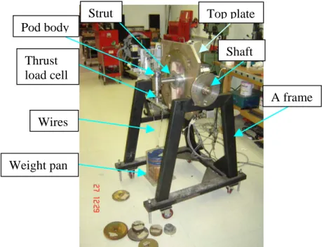
The calibration setup consisted of a steel A frame and a top plate, onto which any of the IOT pod models can be attached. This plate can be rotated 3608 about a horizontal shaft, which is attached to the A frame (9). The thrust load cell and torque strain gauges are at the propeller end of the pod body.

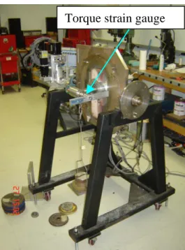
During the calibrations thrust and torque sensors were calibrated in fully assembled pod model as shown in 9and Error! Reference source not found.0. Both sensors were calibrated individually and additional calibration loads applied to determine the cross talk effects, i.e. the interference of each sensor on to the other when loaded. For uniform compression or tension a bar was connected to the load cell. A weight pan was hung from the ends of the bar by a wire to hold the weights. Figure 9 shows the configuration for applying loads to the thrust load cell in tension. For compression mode, the pod body is rotated 1808 about the strut A wooden block was placed between the wires to stop them from touching the sides of the metal block when calibrating in compression. 0 shows the setup for torque calibration. The pan was hung on one side of the bar to create a moment arm about the shaft axis. The moment arm used was 0.0762m (3 in.). When calculating torque one has to be careful because maximum torque can be exceeded easily. The load cell was connected to the Data Acquisition System shown in Figure 8.

Pod body Strut Thrust load cell Shaft A frame Top plate Wires Weight pan

(21)

Torque strain gauge

Figure 10: Thrust Torque Calibration Set-Up, (Torque Applied)

5.1.2 Determining Calibration Equation: Calibration equations used are in the form of

F = CR + C0: where F is the Force acting on the load cell, C is the linear calibration slope, R is the voltage output of the sensor and C0 is the intercept. To determine the calibration equation of a given load cell, known loads are applied to the load cell and the output voltages are recorded for each different load. Loads are applied with the load cell in compression and also in tension (+/- for torque strain gauge) and a linear least squares method is used to fit the data points. Due to nonlinearity around the origin (zero load) an ‘S’ curve was observed in the graphs. This region of nonlinearity was modeled by second or third order polynomials.

To identify the ‘S’ curve more accurately a lighter pan and weights were chosen and the process was repeated. The weights used during the calibrations are given in the table below (Table 1).

The equations obtained for the load cells are: IOT Pod Model A:

• Thrust: T = 491.5629695 R + 3.1996760 • Torque: Q = 0.0112695 R + 0.1112951 IOT Pod Model B:

• Thrust: T = 496.4069012 R + 3.9031931 • Torque: Q = -0.0109452 R + 0.0401382

(22)

Table 3: Weights used in thrust and torque calibrations

Weight # Grams Newtons Weight # Grams Newtons

wooden piece to hold the wires apart 86.4 0.847411 12 4732.8 46.4193

Bar to hold the weight pan + wires + hooks + wooden piece to hold the wires apart

500.7 4.910866 13 4665.2 45.75628

Weight Pan (Pan1) 1502.2 14.73358 14 4629.6 45.40712

5 2038.5 19.99361 15 4688.4 45.98383 6 1997 19.58658 16 4626.2 45.37377 7 995.8 9.766806 Pan2 313.4 3.073827 8 2039.9 20.00734 1 303.2 2.973786 10 2257.8 22.1445 2 453.6 4.448909 11 2458.3 24.11101 3 655.9 6.433067

5.3 Global Dynamometer

5.3.1 Determining Calibration Equation

Similar to calibrating the thrust and torque sensors the load cells on the global

dynamometer had known loads applied and a linear least squares method was used. The calibration equation has the same form as the equations for thrust and torque sensors. The equations obtained for the individual load cells are:

• Fx1a = 34.881835 R + 1.618834 • Fy1a = 34.651073 R + 0.767444 • Fy2a = 35.971403 R - 2.673602 • Fz1a = 34.485942 R - 0.981804 • Fz2a = 35.099573 R + 3.387109 • Fz3a = 36.913956 R - 1.888759 • Fx1b = 35.89327 R - 0.230241 • Fy1b = 35.792136 R + 1.999045 • Fy2b = 34.778186 R + 1.641172 • Fz1b = 37.516834 R - 2.736824 • Fz2b = 35.188171 R + 2.03631 • Fz3b = 35.506041 R + 0.522688

(23)

6.0 Description of Experimental Set Up

The tests were run in NRC-IOT’s Towing Tank. First the model stern was secured to the frame of the carriage. The dynamometer was then put into place and connected to the model stern. The DAS was onboard the carriage and connected to the test apparatus. The propeller was put on the pod after everything was in place. Once everything was in place the propeller was run and a force applied to it to make sure everything was working properly. The unit was then lowered into the water with a draft of 50mm.

(24)

Parts of DAS system

Figure 12: Experimental Set-Up in Towing Tank (2)

7.0 Description of The Experiments

This section describes the various experiments carried out in this project.

7.1 Air Friction Tests

Conducted by running the propeller at various propeller shaft speeds (rps) out of water. These tests are done before any opens tests and at the end of the day when all tests are finished. These tests give an idea of mechanical noise existed in the system.

7.2 Bollard Runs

Conducted when the Carriage is stopped. The propeller is run at various shaft rotational speeds which allow for the computation of Bollard Pull. The Bollard Pull is the amount of thrust produced by the propeller when the vessel’s velocity is zero or near zero. This is important for vessels such as tugboats which operate at low speeds. Bollard runs are also done at very low rps setting i.e. 0.5 rps at the beginning of each test run for tarring purposes. Thrust and torque values obtained at 0.5 rps in this test program were almost negligible.

(25)

7.3 Opens Tests

These tests included static tests with a single pod The characteristic of these tests are that the orientation of the pod is set at angle to the incoming flow, i.e. azimuth angle. To achieve this the pod model was rotated a certain angle about the vertical axis passing through the centre of the strut. During the dynamics tests, the azimuthing angle was varied continuously.

7.3.1 Static Tests

These tests are conducted with azimuthing angles ranging from 0 to 360 degrees, positive and negative propeller speeds ranging from 0.5 to 15 rps, and carriage speeds ranging from 0.2 to 3.6 m/s. The definition of a positive rps is when the propeller rotated at this rps the thrust generated pulls the pod away from the propeller.

.

7.3.2 Dynamic Tests

The pod in these tests were azimuthing between two set angles at given rates ranging from 2 8/s to 20 8/s. Test procedure are similar to the static tests except one must make sure that the torque experienced by the propeller does not exceed a value of 9.6 N-m. These tests were also conducted using dual pods with both pods azimuthing and one pod azimuthing and one pod static.

8.0 Data Analysis

This section will describe the online and offline data analysis and also some results obtained from the experiments. Both the offline and online analysis was done using a segment selection method described below.

8.1 Online Analysis

The online analysis is done while the experiments are being conducted. These results are not final but are used in order to see if the data being collected seem reasonable. Also during runs where torque can exceed its maximum limit the researcher checks torque values to see if more severe test conditions should be carried out. From these test results the researcher can check to see if the test data matches the given coordinate system. If not it can be changed accordingly.

(26)

8.2 Offline Analysis

This analysis is completed after the experiments finished. Few more parameters were also computed during this analysis, such as global moments acting on the pod system.

8.2 Interpreting the Raw Data

The analysis of the data was done using the new Sweet software. A segment selector was used to choose specific sections of each run to analyze. A time series was plotted and the data from the run sequences was interpreted. Obtained in a pdf file were plots of global loads, moments, thrust, and torque versus time and also tables containing mean, min, max, and standard deviation values for each channel of the sensors. The data was also imported into a spreadsheet where they could be further processed.

Figure 13 shows a typical static run sequence in the tank. In the first segment (shaded area) everything is stationary, the carriage velocity, shaft speed RPS, and azimuthing angle are zero. The other segments are tarred with respect to the first segment. The second segment is equivalent to a bollard pull, at 0.5 rps (will be used later for tarring purposes). The third portion of the graph is a bollard pull at 15 rps. The fourth and fifth segments of the graph are for the two carriage velocities.

(27)

Figure 14 shows a typical dynamic run sequence. At this phase of the analysis, the procedure is the same as mentioned above. Note that the dynamic nature of the

azimuthing angle can be seen in the bottom graph. The angles were varied between –35 and +35 degrees.

Figure 14: Typical Dynamic Run Sequence Showing Segments

9.0 Description of Cases

This section will describe the tests carried out at the MUN towing tank and the NRC towing tank. The first two cases are taken from Lane’s Report, A Study On the Scale Effects of Propulsive Characteristics of Podded Propulsors (Lane 2006).

9.1 Case 1

The experiments conducted in January 2005 were on a single podded propeller with a diameter of 270mm - MUN-NRC-NSERC. The following is a list of the types of experiments conducted: Air Friction and Bollard Runs, Opens Tests (0 deg azimuth), Oblique Flow Tests, and Third Quadrant Runs. For comparisons given in this report the results for only 0 deg azimuthing angles were used.

(28)

Table 4: General test plan for Air Friction Tests, Case 1

Air Friction Tests

Mode Pull Mode

RPS 12 (in both positive and negative directions)

Carriage Velocity (m/s) 0

Azimuth Angle (deg) 0

Table 5: General test plan for Bollard Runs, Case 1

Bollard Runs

Mode Pull Mode

RPS -11 to 10

Table 6: General test plan for Opens Tests, Case 1

Opens Tests

Mode Pull Mode

RPS 12

Carriage Velocity (m/s)

0.324, 0.648, 0.972, 1.296, 1.62, 1.944, 2.268, 2.592, 2.916, 3.24, 3.564

9.2 Case 2

This is the numerical results of the same set-up as case 1; and was completed on Oct 24/04. They were computed for a single podded propeller with a 270mm diameter. Mohammed Islam and Dr. Pengfei Liu completed the test using the program PROPELLA.

9.3 Case 3

These are the tests carried out at the NRC-IOT Towing Tank in March 2007 on a single podded propeller. The following is a list of the types of experiments conducted: Air Friction and Bollard Runs, Opens Tests (0 deg azimuth), Oblique Flow Tests, and Third Quadrant Runs.

(29)

Table 7: General test plan for Air Friction Tests, Case 3

Air Friction Tests

Mode Pull Mode

RPS 0.5, 1-16

Table 8: General test plan for Bollard Runs, Case 3

Bollard Runs

Mode Pull Mode

RPS 0.5, 1-16

Table 9:General test plan for Opens Tests, Case 3

Opens Tests

Mode Pull Mode

RPS 15

Carriage Velocity (m/s) 0.6, 1.2, 1.8, 2.1, 2.4, 2.7, 3.0, 3.3, 3.6

(30)

10.0 Comparison of Data

This section will compare the data collected from the tests described above. Used in the comparison are Kt, 10Kq, KFx, KFy, and KFz Results for Kfy and KFz from

PROPELLA were not available.

Single Pod, 0 degrees

-0.2 -0.1 0 0.1 0.2 0.3 0.4 0.5 0.6 0.7 0.8 0 0.2 0.4 0.6 0.8 1 1.2 J Kt, 10Kq, KFx NSERC Kt NSERC 10Kq NSERC KFx IOT Kt IOT 10Kq IOT KFx PROPELLA Kt PROPELLA 10Kq PROPELLA KFx Poly. (NSERC 10Kq) Poly. (NSERC Kt) Poly. (NSERC KFx) Poly. (IOT Kt) Poly. (IOT 10Kq) Poly. (IOT KFx) Poly. (PROPELLA 10Kq) Poly. (PROPELLA KFx)

(31)

Single Pod, 0 degrees

-0.2 -0.1 0 0.1 0.2 0.3 0.4 0.5 0 0.2 0.4 0.6 0.8 1 1.2 J KFx, KFy, KFz NSERC KFz NSERC KFy NSERC KFx IOT KFx IOT KFy IOT KFz

Poly. (NSERC KFy) Poly. (NSERC KFz) Poly. (NSERC KFx) Poly. (IOT KFx) Poly. (IOT KFy) Poly. (IOT KFz)

Figure 16: Comparison of KFx, KFy, KFz

From the above set of plots good comparison can be viewed for Kt, Kq, KFx, KFy, and KFz. All cases go negative between J=1.05 and J=1.1 for KFx. All cases go negative at approximately J=1.2 for 10Kq. All cases go negative between J=1.1 and J=1.15 for Kt. In the plots of KFx, Kfy, and KFz versus J good comparison can be seen between both cases- cases 1 and 3. Kfy and KFz are near zero at the range of speeds tested, which is expected due to the orientation of the model in the water

11.0 Results and Discussion

In the current study of podded propellers the tests were carried out in the NRC-IOT Towing Tank. The propellers were four bladed. The tests were conducted in pull mode at various azimuth angles. The following are some of the results obtained from these opens tests. Due to commercially sensitive data only a sample of what was collected can be shown in this report. For the rest of the data, please contact IOT with reference to Project number 42_2194_16.

(32)

Single Pod, 0 degrees

-0.2 -0.1 0 0.1 0.2 0.3 0.4 0.5 0.6 0.7 0.8 0 0.2 0.4 0.6 0.8 1 1.2 J Kt, 10Kq, KFx Kt 10Kq KFx Poly. (10Kq) Poly. (Kt) Poly. (KFx)

Figure 17: Kt, 10Kq, KFx for NRC-IOT Tests

Single Pod, 0 degrees

-0.2 -0.1 0 0.1 0.2 0.3 0.4 0.5 0 0.2 0.4 0.6 0.8 1 1.2 J KFx, KFy, KFz KFx KFy KFz Poly. (KFy) Poly. (KFx) Poly. (KFz)

(33)

Single Pod, J = 0.4 -0.6 -0.4 -0.2 0 0.2 0.4 0.6 0.8 1 0 50 100 150 200 250 300 350 400 Azimuthing Angle Kt, 10Kq, KFx Kt 10Kq KFx

Figure 19: Kt, 10Kq, KFx vs Azimuthing Angle, at J=0.4

Single Pod, J = 0.8 -0.8 -0.6 -0.4 -0.2 0 0.2 0.4 0.6 0.8 1 1.2 0 50 100 150 200 250 300 350 400 Azimuthing Angle Kt, Kq, KFx Kt 10Kq KFx

(34)

As discussed in the previous section good results can be viewed for Kt, Kq, KFx, KFy, and KFz. Also included here are plots of the coefficients versus azimuthing angles, which also seem reasonable, ranging from 0º to 360º at J=0.4 and J=0.8.

12.0 Recommendations and Conclusions

Overall the tests done at the NRC-IOT with IOT pod model show comparisons with previously published data. The quality of the data generated during the experiments seems very good. With these new tests, the definition of the performance envelop of podded propulsors is increased. Further testing plans include the building of a model vessel where model self-propulsion tests will be conducted.

Before conducting future tests consideration should be given to calibrating the global load cells to allow for the determination of interaction effects.

13.0 Acknowledgements

I would like to take this opportunity to express my gratitude to all those who in any way contributed to the positive experience of this work term. Firstly I would like to thank the National Research Council for giving me the opportunity to work at a world-class

research facility. Thank you to the staff at the NRC-IOT towing tank and work shops for their support and assistance. I want to thank Mohammad Islam (Shameem) for his

assistance. Finally I would like to thank Dr. Ayhan Akinturk for his support and guidance during my work term, which allowed me to augment my engineering education.

(35)

14.0 References

1) National research Council of Canada – Institute for Ocean Technology website. URL:

http://iot-ito.nrc-cnrc.gc.ca/facilities/

2) Ocean Consulting Corporation Website>Facilities>58m Towing Tank. URL:

http://www.oceaniccorp.com/FacilityDetails.asp?id=2

3) Islam, M., Veitch, B., Bose, N., Liu, P., (2006). “Hydrodynamic Characteristics of Puller Podded Propulsors with Tapered Hub Propellers.”

4) Bell, J., (2005). “TDC Podded Propeller Drive.” Institute for Ocean Technology, NRC: Report No. LM –2005-01

5) MacNeil, A., Taylor, R., Malloy, S., Bose, N., Veitch, B., Randell, T., Liu, P., (2004). “Design of Model Pod Test Unit.” Proceedings of the 1st International Conference on Technological Advances in Podded Propulsion. Newcastle University, UK, April. 6) Lane, S., (2006). “A Study On the Scale Effects of Propulsive Characteristics of Podded Propulsors.”

(36)

(37)

Calibrated 03-May-2006 09:58

National Research Council Canada

Test Facility: Tow Tank Serial #: Filter Frequency:

Data Source: DASPC13 Channel 1 Programmable Gain: 1 Excitation Voltage:

Sensor Model: Plug-In Gain:

Data Physical Measured Fitted Curve Error

Point Value Value Value Definition of Calibration Curve

# (deg) (counts) (deg) (deg)

1 0.00000 0.00000 -0.0011208 -0.0011208 Polynomial Degree = 1 (Linear Fit) 2 20.000 3641.0 20.000 -0.00013064 Y = C0 + C1 · V

3 45.000 8192.0 45.000 -0.00026628 where Y(t) = Angle (deg),

4 90.000 16384. 90.001 0.00058821 V(t) = measured value (counts),

5 180.00 32768. 180.00 0.0022972 C0 = -0.0011208 deg, 6 315.00 57343. 315.00 -0.00063260 C1 = 0.0054933 deg/count. 7 340.00 61894. 340.00 -0.00076824

(38)

# (deg) (counts) (deg) (deg)

1 18153. 18153. 18153. 0.00000 Polynomial Degree = 1 (Linear Fit) 2 62389. 62389. 62389. 0.00000 Y = C0 + C1 · V

where Y(t) = Angle (deg),

V(t) = measured value (counts), C0 = 0 deg,

(39)

# (rps) (counts) (rps) (rps)

1 -13.000 2340.6 -13.000 1.2530e-005 Polynomial Degree = 1 (Linear Fit) 2 -7.5000 15214. -7.5000 1.3001e-005 Y = C0 + C1 · V

3 -4.0000 23405. -4.0000 -1.2454e-006 where Y(t) = Angular Velocity (rps), 4 1.0000 35108. 0.99997 -2.5889e-005 V(t) = measured value (counts),

5 4.0000 42130. 4.0000 -1.9146e-005 C0 = -14 rps,

6 7.5000 50322. 7.5000 -1.2948e-005 C1 = 0.00042725 rps/count. 7 13.000 63195. 13.000 3.4462e-005

(40)

# (volts) (counts) (volts) (volts)

1 -4.5000 18087. -4.5001 -0.00010798 Polynomial Degree = 1 (Linear Fit) 2 -2.5000 24630. -2.5001 -8.1337e-005 Y = C0 + C1 · V

3 0.00000 32811. 0.00043507 0.00043507 where Y(t) = Voltage (volts),

4 2.5000 40989. 2.4998 -0.00020963 V(t) = measured value (counts),

5 4.5000 47533. 4.5000 -3.6725e-005 C0 = -10.028 volts,

(41)

Calibrated 14-Mar-2006 11:32

Test Facility: Tow Tank Serial #: E50407 Filter Frequency: 1000

Data Source: PC004026 Channel 1 Programmable Gain: 1 Excitation Voltage:

# (volts) (volts) (volts) (volts)

1 -0.030000 -4.5012 -0.030000 5.3259e-008 Polynomial Degree = 1 (Linear Fit) 2 -0.015000 -2.2533 -0.015001 -1.1223e-006 Y = C0 + C1 · V

3 0.00000 -0.0048398 9.8631e-007 9.8631e-007 where Y(t) = Voltage (volts), 4 0.015000 2.2433 0.015001 1.1843e-006 V(t) = measured value (volts),

5 0.030000 4.4911 0.029999 -1.1016e-006 C0 = 3.3278e-005 volts,

(42)

1 -0.030000 -4.4996 -0.030001 -5.9333e-007 Polynomial Degree = 1 (Linear Fit) 2 -0.015000 -2.2529 -0.015001 -1.1858e-006 Y = C0 + C1 · V

5 0.030000 4.4873 0.029997 -2.5527e-006 C0 = 3.9454e-005 volts,

(43)

5 0.030000 4.4885 0.029996 -3.5259e-006 C0 = 2.1934e-005 volts,

(44)

5 0.030000 4.4863 0.029997 -3.4165e-006 C0 = 4.2599e-005 volts,

(45)

5 0.030000 4.4863 0.029998 -1.8883e-006 C0 = 2.7784e-005 volts,

(46)

5 0.030000 4.4910 0.029997 -2.8285e-006 C0 = 4.1689e-005 volts,

(47)

Calibrated 28-Feb-2007 12:00

Test Facility: Tow Tank Serial #: 14381 Filter Frequency: 1000

1 -0.80000 -3.8610 -0.79999 1.3797e-005 Polynomial Degree = 1 (Linear Fit) 2 -0.50000 -2.4140 -0.50004 -3.9630e-005 Y = C0 + C1 · V

5 0.80000 3.8576 0.79997 -2.7413e-005 C0 = 0.00034603 volts,

(48)

Test Facility: Tow Tank Serial #: A Filter Frequency: 1000

3 0.00000 -0.0048058 1.9123e-005 1.9123e-005 where Y(t) = Voltage (volts), 4 0.50000 2.7152 0.50000 -4.8153e-006 V(t) = measured value (volts),

5 0.80000 4.3472 0.80000 -4.0548e-006 C0 = 0.00090251 volts,

(49)

Not Calibrated

(50)

Test Facility: Tow Tank Serial #: Filter Frequency: 10

Data Source: TOWDAS Channel 3 Programmable Gain: 1 Excitation Voltage:

Sensor Model: Carriage laser position output Plug-In Gain: 1

# (mm) (volts) (mm) (mm)

1 10000. -9.0033 9999.4 -0.63455 Polynomial Degree = 1 (Linear Fit) 2 1.0000e+005 -0.0040650 1.0000e+005 1.2675 Y = C0 + C1 · V

3 1.9000e+005 8.9948 1.9000e+005 -0.63671 where Y(t) = Displacement (mm),

V(t) = measured value (volts), C0 = 1.0004e+005 mm,

(51)

Calibrated 15-Jan-2007 11:10

Test Facility: Tow Tank Serial #: Filter Frequency: 10

Data Source: TOWDAS Channel 33 Programmable Gain: 1 Excitation Voltage: 10

Sensor Model: Plug-In Gain: 1

# (m/s) (volts) (m/s) (m/s)

1 -0.62500 -9.0052 -0.62504 -4.1415e-005 Polynomial Degree = 1 (Linear Fit) 2 2.7500 -0.0011765 2.7501 8.2813e-005 Y = C0 + C1 · V

3 6.1250 9.0022 6.1250 -4.1682e-005 where Y(t) = Velocity (m/s),

V(t) = measured value (volts), C0 = 2.7505 m/s,

(52)

Test Facility: Tow Tank Serial #: 200282 Filter Frequency: 10

Data Source: TOWDAS Channel 34 Programmable Gain: 1 Excitation Voltage: 10

Sensor Model: Celesco PT101-0050-111-1130 Plug-In Gain: 1

# (mm) (volts) (mm) (mm)

1 0.00000 0.36430 0.053916 0.053916 Polynomial Degree = 1 (Linear Fit) 2 100.00 1.0997 100.20 0.19569 Y = C0 + C1 · V

3 200.00 1.8305 199.72 -0.27975 where Y(t) = Displacement (mm), 4 300.00 2.5663 299.93 -0.071887 V(t) = measured value (volts),

5 400.00 3.3012 400.00 0.0020918 C0 = -49.558 mm, 6 500.00 4.0360 500.08 0.076298 C1 = 136.18 mm/volt. 7 600.00 4.7696 599.98 -0.023104

(53)

(54)

DATE E TIME(mins) FILENAME(.DAC) RUN DESCRIPTION COMMENTS Required Actual Shaft Speed Pod A(RPS) Carriage Vs.(m/s) Azimuthing Angle Pod A

POD A (PORT) ONLY

Mar-01-2007 9:02 10 2:06 Zero_001 0 0.0 n/a

" 11:08 10 0:24 Frictions_001 0.5, 1-16 0.0 Morning Frictions - positive rps

" 11:32 10 1:28 Ckeck_rps_001 10 0.0 no video

" 13:00 10 1:00 Air_Friction_001 0.5, 1-16 0.0

Morning Frictions - positive rps. Annotator not updated

14:00 10 0:12 Bollard_001 0.5, 1-16 0.0 Video started late.

" 14:12 10 0:15 APS_322L_Static_001 -15 0.6,1.2,1.8,2.1 0 positive rps " 14:27 10 0:44 APS_322L_Static_002 -15 0.6,1.2,1.8,2.1 0 positive rps, repeat

" 15:11 10 0:12 APS_322L_Static_003 -15 2.4,2.7 0 "

" 15:23 10 0:09 APS_322L_Static_004 -15 3.0 0 ", Annotator not updated

" 15:32 10 0:09 APS_322L_Static_005 -15 3.3 0 " " 15:41 10 0:11 APS_322L_Static_006 -15 3.6 0 " " 15:52 10 0:11 APS_322L_Static_007 -15 0.6,1.2,1.8,2.1 5 " " 16:03 10 0:10 APS_322L_Static_008 -15 2.4,2.7 5 " " 16:13 10 0:08 APS_322L_Static_009 -15 3.0 5 " " 16:21 10 0:08 APS_322L_Static_010 -15 3.3 5 " " 16:29 10 0:17 APS_322L_Static_011 -15 3.6 5 "

" 16:46 10 ##### Air_Friction_002 0.5, 1-16 0.0 0 Evening Frictions - positive rps

02-Mar-07 8:19 10 0:47 Air_Friction_003 0.5, 1-16 0.0 0

Morning Frictions - positive rps -- No Connection to PC004026 -- Restart DAS

" 9:01 10 0:05 APS_322L_Static_012 0.5 0.0 -5 Tare Run 0.5 RPS

" 9:06 10 0:10 APS_322L_Static_013 -15 0.6,1.2,1.8,2.1 -5 "

" 9:16 10 0:10 APS_322L_Static_014 -15 2.4,2.7 -5 Roughing

" 9:26 10 0:10 APS_322L_Static_015 -15 3.0 -5 "

" 9:36 10 0:10 APS_322L_Static_016 -15 3.3 -5 "

(55)

" 10:53 10 0:10 APS_322L_Static_021 -15 3.0 10

New Control Program Loaded (0.5 RPS At Beginning of every Run) " 11:03 10 0:10 APS_322L_Static_022 -15 3.3 10 Annotator Read 23 (Should Have Been 22)

" 11:13 10 0:11 APS_322L_Static_023 -15 3.6 10 " " 11:24 10 0:10 APS_322L_Static_024 -15 0.6,1.2,1.8,2.1 -5 Repeat " 11:34 10 0:11 APS_322L_Static_025 -15 2.4,2.7 -5 Repeat " 11:45 10 0:10 APS_322L_Static_026 -15 0.6,1.2,1.8,2.1 -10 " " 11:55 10 0:10 APS_322L_Static_027 -15 2.4,2.7 -10 " " 12:05 10 0:10 APS_322L_Static_028 -15 3.0 -10 " " 12:15 10 0:10 APS_322L_Static_029 -15 3.3 -10 " " 12:25 10 1:04 APS_322L_Static_030 -15 3.6 -10 " " 13:29 10 0:10 APS_322L_Static_031 -15 0.6,1.2,1.8,2.1 15 " " 13:39 10 0:17 APS_322L_Static_032 -15 2.4,2.7 15 "

" 13:56 10 0:10 APS_322L_Static_033 -15 3.0 15 Re-Run - Forgot to Start Props

" 14:06 10 0:10 APS_322L_Static_034 -15 3.3 15 " " 14:16 10 0:10 APS_322L_Static_035 -15 3.6 15 " " 14:26 10 0:10 APS_322L_Static_036 -15 0.6,1.2,1.8,2.1 -15 " " 14:36 10 0:10 APS_322L_Static_037 -15 2.4,2.7 -15 " " 14:46 10 0:10 APS_322L_Static_038 -15 3.0 -15 " " 14:56 10 0:10 APS_322L_Static_039 -15 3.3 -15 " " 15:06 10 0:10 APS_322L_Static_040 -15 3.6 -15 "

" 15:16 10 0:12 APS_322L_Static_041 -15 0.6,1.2,1.8,2.1 20 Annotator not updated

" 15:28 10 0:10 APS_322L_Static_042 -15 2.4,2.7 20 Annotator updated part ways through run.

" 15:38 10 0:08 APS_322L_Static_043 -15 3.0 20 " " 15:46 10 0:08 APS_322L_Static_044 -15 3.3 20 " " 15:54 10 0:10 APS_322L_Static_045 -15 3.6 20 " " 16:04 10 0:11 APS_322L_Static_046 -15 0.6,1.2,1.8,2.1 -20 " " 16:15 10 0:08 APS_322L_Static_047 -15 2.4,2.7 -20 " " 16:23 10 0:07 APS_322L_Static_048 -15 3.0 -20 " " 16:30 10 0:07 APS_322L_Static_049 -15 3.3 -20 " " 16:37 10 ##### APS_322L_Static_050 -15 3.6 -20 " " 10 0:00 n/a 0.5, 1-16 0.0 0

Can't start software to do frictions! Evening Frictions - positive rps

(56)

" 8:05 10 0:22 APS_322L_Static_051 -15 2.4,2.7 30

Set Prop to Start Position - Lower Test Frame - Rough Up Run (2 Speeds)

" 8:27 10 0:10 APS_322L_Static_052 -15 2.4,2.7 30 Rough Up

" 8:37 10 0:10 APS_322L_Static_053 -15 0.6,1.2,1.8,2.1 30 Annotator Not Updated

" 8:47 10 0:10 APS_322L_Static_054 -15 2.4,2.7 30 " " 8:57 10 0:10 APS_322L_Static_055 -15 3.0 30 " " 9:07 10 0:10 APS_322L_Static_056 -15 3.3 30 " " 9:17 10 0:10 APS_322L_Static_057 -15 3.6 30 " " 9:27 10 0:10 APS_322L_Static_058 -15 0.6,1.2,1.8,2.1 -30 " " 9:37 10 0:10 APS_322L_Static_059 -15 2.4,2.7 -30 " " 9:47 10 0:10 APS_322L_Static_060 -15 3.0 -30 " " 9:57 10 0:10 APS_322L_Static_061 -15 3.3 -30 " " 10:07 10 0:49 APS_322L_Static_062 -15 3.6 -30 "

" 10:56 10 0:10 APS_322L_Dyn_200 -8 0.6 (-35-35) Dynamic Azimuthing Runs (Rate:2°/sec)

" 11:06 10 0:10 APS_322L_Dyn_201 -8 1.2 (-35-35) " " 11:16 10 0:10 APS_322L_Dyn_202 -8 1.8 (-35-35) " " 11:26 10 0:10 APS_322L_Dyn_203 -8 2.1 (-35-35) " " 11:36 10 0:10 APS_322L_Dyn_204 -8 2.4 (-35-35) " " 11:46 10 1:10 APS_322L_Dyn_205 -8 2.7 (-35-35) " " 12:56 10 0:10 APS_322L_Dyn_206 -8 3.0 (-35-35) " " 13:06 10 0:10 APS_322L_Dyn_207 -8 3.3 (-35-35) " " 13:16 10 0:10 APS_322L_Dyn_208 -8 3.6 (-35-35) " " 13:26 10 0:10 -8 0.6-1.2 (-35-35)

Dynamic Azimuthing Runs (Rate:5°/sec) - GDAC Crashed - No Data Downloaded

" 13:36 10 0:11 APS_322L_Dyn_209 -8 0.6-1.2 (-35-35) Repeat

" 13:47 10 0:09 APS_322L_Dyn_210 -8 1.8 (-35-35) "

" 13:56 10 0:11 APS_322L_Dyn_211 -8 1.8, 2.1 (-35-35) "

" 14:07 10 0:10 APS_322L_Dyn_212 -8 2.4 (-35-35) "

" 14:17 10 0:10 APS_322L_Dyn_213 -8 0.32, 1.28, 1.6 (-35-35) "

" 14:27 10 0:09 APS_322L_Dyn_214 -8 0.32,0.8,1.12 (-35-35) Azimuthing rate now 10 deg/sec " 14:36 10 0:10 APS_322L_Dyn_215 -8 0.32,0.8,1.12 (-35-35) repeat

(57)

" 15:14 10 0:09 APS_322L_Dyn_219 -8 1.28,1.44 (-35-35) "

" 15:23 10 0:08 APS_322L_Dyn_220 -8 1.6 (-35-35) "

" 15:31 10 0:10 APS_322L_Dyn_221 -8 0.32,0.8,1.12 (-35-35) Azimuthing rate now 20 deg/sec

" 15:41 10 0:10 APS_322L_Dyn_222 -8 1.28,1.44 (-35-35) "

" 15:51 10 0:09 APS_322L_Dyn_223 -8 1.6 (-35-35) "

" 16:00 10 0:11 APS_322L_Dyn_224 -15 0.6, 1.5 (-35-35)

Azimuthing rate now 2 deg/sec, constant speed not long enough -- increase run

distance and repeat " 16:11 10 0:10 APS_322L_Dyn_225 -15 0.6, 1.5 (-35-35) Azimuthing rate now 2 deg/sec

" 16:21 10 0:12 APS_322L_Dyn_226 -15 2.1 (-35-35) "

" 16:33 10 0:21 Air_Friction_005 0.5, 1-16 0.0 0

Evening Frictions - positive rps, Annotator not updated. GDAC crashed - no data.

" 16:54 10 ##### Zero_003 0 0.0 0 zeros at the end of the day

07-Mar-07 7:10

Set-up DAS and Model - Set Prop to Start Position

" 7:25 10 0:28 Air_Friction_006 0.5, 1-16 0.0 0 Morning Frictions - positive rps

" 7:53 10 0:10 APS_322L_Dyn_227 -15 2.4 (-35-35) Rough Up

" 8:03 10 0:10 APS_322L_Dyn_228 -15 2.4 (-35-35) Rough Up

" 8:13 10 0:10 APS_322L_Dyn_229 -15 2.4 (-35-35) "

" 8:23 10 0:10 APS_322L_Dyn_230 -15 2.7 (-35-35) "

" 8:33 10 0:12 APS_322L_Dyn_231 -15 3.0 (-35-35) "

" 8:45 10 0:10 APS_322L_Dyn_408 -15 0.6, 1.5 (-35-35) Azimuthing Rate (5°/s) " 8:55 10 0:10 APS_322L_Dyn_409 -15 2.1 (-35-35) Annotator was not updated for this run

" 9:05 10 0:10 APS_322L_Dyn_410 -15 2.4 (-35-35) "

" 9:15 10 0:10 APS_322L_Dyn_411 -15 2.7 (-35-35) "

" 9:25 10 0:10 APS_322L_Dyn_412 -15 3.0 (-35-35) "

" 9:35 10 0:12 APS_322L_Dyn_413 -15 0.6, 1.5 (-35-35) Azimuthing Rate (10°/s)

" 9:47 10 0:10 APS_322L_Dyn_414 -15 2.1 (-35-35) "

" 9:57 10 0:10 APS_322L_Dyn_415 -15 2.4 (-35-35) "

" 10:07 10 0:13 APS_322L_Dyn_416 -15 2.7 (-35-35) "

" 10:20 10 0:36 APS_322L_Dyn_417 -15 3.0 (-35-35) "

" 10:56 10 0:06 APS_322L_Dyn_Rate_001 -15 0.0 (-35-35) Bollard (Azi. Rate: 0.5°/sec) " 11:02 10 0:14 APS_322L_Dyn_Rate_002 -15 0.0 (-35-35) Bollard (Azi. Rate: 0.5°/sec)

(58)

" 11:36 10 0:06 APS_322L_Dyn_Rate_006 -15 0.0 (-35-35) Bollard (Azi. Rate: 15°/sec) " 11:42 11 1:33 APS_322L_Dyn_Rate_007 -15 0.0 (-35-35) Bollard (Azi. Rate: 20°/sec) " 13:15 10 0:10 APS_322L_Dyn_418 -15 0.6, 1.5 (-35-35) Azimuthing Rate (15°/s)

" 13:25 10 0:10 APS_322L_Dyn_419 -15 2.1 (-35-35) "

" 13:35 10 0:10 APS_322L_Dyn_420 -15 2.4 (-35-35) "

" 13:45 10 0:10 APS_322L_Dyn_421 -15 2.7 (-35-35) "

" 13:55 10 0:10 APS_322L_Dyn_422 -15 3.0 (-35-35) "

" 14:05 10 0:10 APS_322L_Dyn_423 -15 0.6, 1.5 (-35-35) Azimuthing Rate (20°/s)

" 14:15 10 0:10 APS_322L_Dyn_424 -15 2.1 (-35-35) "

" 14:25 10 0:10 APS_322L_Dyn_425 -15 2.4 (-35-35) "

" 14:35 10 0:10 APS_322L_Dyn_426 -15 2.7 (-35-35) "

" 14:45 10 0:16 APS_322L_Dyn_427 -15 3.0 (-35-35) "

" 15:01 10 0:05 Bollard_002 -15 0.0 0 Bollard 15 RPS; 0°

" 15:06 10 0:27 APS_322L_Static_067 -15 0.6,1.2,1.8,2.1 60 Static Case 60°

" 15:33 10 0:09 APS_322L_Static_068 -15 2.4,2.7 60 "

" 15:42 10 0:08 APS_322L_Static_069 -15 3.0 60 "

" 15:50 10 0:09 APS_322L_Static_070 -15 3.3 60 "

" 15:59 10 0:10 APS_322L_Static_071 -15 3.6 60 "

" 16:09 10 0:10 APS_322L_Static_072 -15 0.6,1.2,1.8,2.1 -60 Static Case -60°

" 16:19 10 0:09 APS_322L_Static_073 -15 2.4,2.7 -60 "

" 16:28 10 0:09 Air_Friction_007 0.5, 1-16 0.0 0 Evening Frictions - positive rps

08-Mar-07 7:30 10 0:16 Air_Friction_008 0.5, 1-16 0.0 0

Set Prop to Start Position - Morning Frictions - positive rps " 7:46 10 0:10 APS_322L_Static_074 -15 2.4,2.7 30

-- Lower Test Frame - Rough Up Run (2 Speeds)

" 8:07 10 0:10 APS_322L_Static_076 -15 3.0 -60

" 8:17 10 0:10 APS_322L_Static_077 -15 3.3 -60

" 8:27 10 0:16 APS_322L_Static_078 -15 3.6 -60

" 8:43 10 0:10 APS_322L_Dyn_236 -8 0.6 (-65-65) Azimuthing Rate (2°/s)

" 8:53 10 0:10 APS_322L_Dyn_237 -8 1.5 (-65-65) "

" 9:03 10 0:10 APS_322L_Dyn_238 -8 2.1 (-65-65) "

(59)

" 10:10 10 0:11 APS_322L_Dyn_243 -8 1.28,1.44 (-65-65) " 10:21 10 0:08 APS_322L_Dyn_244 -8 1.6 (-65-65)

" 10:29 10 0:12 APS_322L_Dyn_245 -8 0.32,0.8 (-65-65) Azimuthing Rate (2°/s) " 10:41 10 0:10 APS_322L_Dyn_246 -8 1.1 (-65-65)

" 10:51 10 0:09 APS_322L_Dyn_247 -8 0.32,0.8,1.12 (-65-65) Azimuthing Rate (10°/s) " 11:00 10 0:17 APS_322L_Dyn_248 -8 1.28,1.44 (-65-65)

" 11:17 10 0:08 APS_322L_Dyn_249 -8 1.6 (-65-65)

" 11:25 10 0:10 APS_322L_Dyn_250 -8 0.32,0.8,1.12 (-65-65) Azimuthing Rate (15°/s) " 11:35 10 0:10 APS_322L_Dyn_251 -8 1.28,1.44 (-65-65)

" 11:45 10 0:44 APS_322L_Dyn_252 -8 1.6 (-65-65)

" 12:29 10 0:10 APS_322L_Dyn_253 -8 0.32,0.8,1.12 (-65-65)

Azimuthing Rate (20°/s), Annotator not updated, Test description incorrect " 12:39 10 0:10 APS_322L_Dyn_254 -8 1.28,1.44 (-65-65)

" 12:49 10 0:17 APS_322L_Dyn_255 -8 1.6 (-65-65) " 13:06 10 0:11 APS_322L_Dyn_428 -15 0.6 (-65-65)

Azimuthing Rate (2°/s), Test description incorrect " 13:17 10 0:11 APS_322L_Dyn_429 -15 1.5 (-65-65) " 13:28 10 0:12 APS_322L_Dyn_430 -15 2.1 (-65-65) " 13:40 10 0:10 APS_322L_Dyn_431 -15 2.4 (-65-65) " 13:50 10 0:12 APS_322L_Dyn_432 -15 2.7 (-65-65) " 14:02 10 0:19 APS_322L_Dyn_433 -15 3.0 (-65-65)

" 14:21 10 0:08 APS_322L_Dyn_434 -15 0.6 (-65-65) Azimuthing Rate (5°/s) " 14:29 10 0:09 APS_322L_Dyn_435 -15 1.5 (-65-65) " 14:38 10 0:10 APS_322L_Dyn_436 -15 2.1 (-65-65) " 14:48 10 0:13 APS_322L_Dyn_437 -15 2.4 (-65-65) " 15:01 10 0:10 APS_322L_Dyn_438 -15 2.7 (-65-65) " 15:11 10 0:26 APS_322L_Dyn_439 -15 3.0 (-65-65) " 15:37 10 0:10 APS_322L_Dyn_440 -15 0.6,1.5 (-65-65)

Azimuthing Rate (10°/s), When azimuthing started it went in wrong direction. Get set was pressed and the angle was noted to be -65. Run aborted and data file deleted. Try again. This

(60)

" 16:14 10 0:10 APS_322L_Dyn_444 -15 3.0 (-65-65)

" 16:24 10 0:09 APS_322L_Dyn_445 -15 0.6,1.5 (-65-65) Azimuthing Rate (15°/s) " 16:33 10 0:09 APS_322L_Dyn_446 -15 2.1 (-65-65)

" 16:42 10 0:09 Air_Friction_009 0.5, 1-16 0.0 0 Evening Frictions - positive rps, no video

09-Mar-07 7:36 10 0:14 Air_Friction_010 0.5, 1-16 0.0 0

-- Lower Test Frame - Rough Up Run (2 Speeds) " 9:11 10 0:10 APS_322L_Static_080 -15 2.4,2.7 30 Rough Up " 9:21 10 0:09 APS_322L_Static_081 -15 2.4,2.7 30 Rough Up " 9:30 10 0:09 APS_322L_Dyn_447 -15 2.4 (-65-65) " 9:39 10 0:09 APS_322L_Dyn_448 -15 2.7 (-65-65) " 9:48 10 0:15 APS_322L_Dyn_449 -15 3.0 (-65-65)

" 10:03 10 0:11 APS_322L_Dyn_450 -15 0.6,1.5 (-65-65) Azimuthing Rate (20°/s) " 10:14 10 0:10 APS_322L_Dyn_451 -15 2.1, 2.4 (-65-65)

" 10:24 10 0:07 APS_322L_Dyn_452 -15 2.7 (-65-65) " 10:31 10 0:10 APS_322L_Dyn_453 -15 3.0 (-65-65)

" 10:41 10 0:11 APS_322L_Static_082 -15 0.6,1.2,1.8,2.1 90 Static Case 90° " 10:52 10 0:09 APS_322L_Static_083 -15 2.4,2.7 90

" 11:01 10 0:11 APS_322L_Static_084 -15 3.0 90

" 11:12 10 0:07 APS_322L_Static_085 -15 0.3,0.9,1.5 90

" 11:19 10 0:10 APS_322L_Static_086 -15 0.6,1.2,1.8,2.1 -90 Static Case -90° " 11:29 10 0:09 APS_322L_Static_087 -15 2.4,2.7 -90

" 11:38 10 0:09 APS_322L_Static_088 -15 3.0 -90

" 11:47 10 0:07 APS_322L_Static_089 -15 0.3,0.9,1.5 -90

" 11:54 10 1:19 APS_322L_Static_090 -15 0.45,0.75,1.05,1.35 90 Static Case 90° " 13:13 10 0:11 APS_322L_Static_091 -15 0.6,1.2,1.8,2.1 120 Static Case 120° " 13:24 10 0:10 APS_322L_Static_092 -15 2.4,2.7 120

" 13:34 10 0:07 APS_322L_Static_093 -15 0.3,0.9,1.5 120

" 13:41 10 0:13 APS_322L_Static_094 -15 0.6,1.2,1.8,2.1 -120 Static Case -120° " 13:54 10 0:11 APS_322L_Static_095 -15 0.3,0.9,1.5 -120

" 14:05 10 0:16 APS_322L_Static_096 -15 0.3,0.6,0.9,1.2,1.5 150 Static Case 150° " 14:21 10 0:18 APS_322L_Static_097 -15 1.8,2.1 150

(61)

" 15:06 10 0:10 APS_322L_Static_101 -15 2.4 150 Static Case 150° " 15:16 10 0:11 APS_322L_Static_102 -15 0.6,1.2,1.8,2.1 45 Static Case 45°

" 15:27 10 0:10 APS_322L_Static_103 -15 2.4,2.7 45 "

" 15:37 10 0:07 APS_322L_Static_104 -15 3.0 45 "

" 15:44 10 0:08 APS_322L_Static_105 -15 3.3 45 "

" 15:52 10 0:07 APS_322L_Static_106 -15 3.6 45 "

" 15:59 10 0:09 APS_322L_Static_107 -15 0.6,1.2,1.8,2.1 -45 Static Case -45° " 16:08 10 0:15 APS_322L_Static_108 -15 2.4,2.7 -45 Towdas crashed

" 16:23 10 0:07 APS_322L_Static_109 -15 3.0 -45 "

" 16:30 10 0:07 APS_322L_Static_110 -15 3.3 -45 "

" 16:37 10 0:05 APS_322L_Static_111 -15 3.6 -45 "

" 16:42 10 0:08 Air_Friction_011 0.5, 1-16 0.0 0 Evening Frictions - positive rps, no video

12-Mar-07 7:14 10 0:17 Air_Friction_012 0.5, 1-16 0.0 0

-- Lower Test Frame - Rough Up Run (2 Speeds)

" 7:41 10 ##### APS_322L_Static_113 -15 2.4,2.7 30 Rough Up

" 10 11:30 -15 2.4,2.7 30

Clock Syncronization Issues -- Doug Walsh & Keith Mews Woring On

Problem For Most of Morning

" 11:40 10 0:12 APS_322L_Static_115 -15 0.6 180 Static Case 180°

" 11:52 10 0:14 APS_322L_Static_116 -15 0.3,0.9 180 "

" 12:06 10 0:13 APS_322L_Static_117 -15 0.45,0.75,1.05 180 "

" 12:19 10 1:12 APS_322L_Static_118 -15 1.2 181 "

" 13:31 10 0:10 APS_322L_Static_119 -15 0.3,0.45,0.75,0.9 175 Static Case 175°

" 13:41 10 0:10 APS_322L_Static_120 -15 1.05,1.2 175 "

" 13:51 10 0:19 APS_322L_Static_121 -15 0.3,0.45,0.75,0.9 -175 Static Case -175°

" 14:10 10 0:10 APS_322L_Static_122 -15 1.05,1.2 -175 "

" 14:20 10 0:10 APS_322L_Static_123 -15 0.3,0.45,0.75,0.9 170 Static Case 170°

" 14:30 10 0:10 APS_322L_Static_124 -15 1.05,1.2 170 "

Performance of podded propulsors in opens tests

Performance of Podded Propulsors in Opens Test

Table of Contents

List of Tables

List of Figures

List of Appendices

Appendix A: Calibration Data

Appendix B: Run Log

1.0 Introduction

2.0 Description of Facilities

2.1 Description of NRC-IOT Towing Tank

3.0 Description of Models

3.1 Description of NRC-IOT Physical Model

3.2 Description of the MUN-NRC-NSERC Pod Model

4.0 Description of Instrumentation

4.1 NRC-IOT Dynamometer

4.2 The MUN-NRC-NSERC Pod Dynamometer

4.3 Model Stern

4.4 Data Acquisition System (DAS) for IOT Pod Model Tests

5.0 Calibrations

[ C ] = [ L ] [ a ]

( [ a ] [ a ]

)

5.1 Thrust and Torque Load Cells

5.3 Global Dynamometer

6.0 Description of Experimental Set Up

7.0 Description of The Experiments

7.1 Air Friction Tests

7.2 Bollard Runs

7.3 Opens Tests

8.0 Data Analysis

8.1 Online Analysis

8.2 Offline Analysis

8.2 Interpreting the Raw Data

9.0 Description of Cases

9.1 Case 1

9.2 Case 2

9.3 Case 3

10.0 Comparison of Data

Single Pod, 0 degrees

Single Pod, 0 degrees

11.0 Results and Discussion

Single Pod, 0 degrees

12.0 Recommendations and Conclusions

13.0 Acknowledgements

14.0 References

POD A (PORT) ONLY