Publisher’s version / Version de l'éditeur:
Vous avez des questions? Nous pouvons vous aider. Pour communiquer directement avec un auteur, consultez la première page de la revue dans laquelle son article a été publié afin de trouver ses coordonnées. Si vous n’arrivez pas à les repérer, communiquez avec nous à [email protected].
Questions? Contact the NRC Publications Archive team at
[email protected]. If you wish to email the authors directly, please see the first page of the publication for their contact information.
https://publications-cnrc.canada.ca/fra/droits
L’accès à ce site Web et l’utilisation de son contenu sont assujettis aux conditions présentées dans le site LISEZ CES CONDITIONS ATTENTIVEMENT AVANT D’UTILISER CE SITE WEB.
Advances in Artificial Intelligence: 23rd Canadian Conference on Artificial
Intelligence, Canadian AI 2010, Ottawa, Canada, May 31 – June 2, 2010.
Proceedings, Lecture Notes in Computer Science; no. 6085, pp. 232-243,
2010-06-02
READ THESE TERMS AND CONDITIONS CAREFULLY BEFORE USING THIS WEBSITE.
https://nrc-publications.canada.ca/eng/copyright
NRC Publications Archive Record / Notice des Archives des publications du CNRC :
https://nrc-publications.canada.ca/eng/view/object/?id=77119b1a-8896-465f-a80f-d201f5f789d8
https://publications-cnrc.canada.ca/fra/voir/objet/?id=77119b1a-8896-465f-a80f-d201f5f789d8
NRC Publications Archive
Archives des publications du CNRC
For the publisher’s version, please access the DOI link below./ Pour consulter la version de l’éditeur, utilisez le lien DOI ci-dessous.
https://doi.org/10.1007/978-3-642-13059-5_23
Access and use of this website and the material on it are subject to the Terms and Conditions set forth at
Robustness of classifiers to changing environments
Environments
Houman Abbasian1, Chris Drummond2, Nathalie Japkowicz1and Stan
Matwin1,3
1
School of Information Technology and Engineering, University of Ottawa
Ottawa, Ontario, Canada, K1N 6N5
[email protected],[email protected],[email protected]
2
Institute for Information Technology, National Research Council of Canada, Ottawa, Ontario, Canada, K1A 0R6
3
Institute of Computer Science, Polish Academy of Sciences, Warsaw, Poland
Abstract. In this paper, we test some of the most commonly used classi-fiers to identify which ones are the most robust to changing environments. The environment may change over time due to some contextual or def-initional changes. The environment may change with location. It would be surprising if the performance of common classifiers did not degrade with these changes. The question, we address here, is whether or not some types of classifier are inherently more immune than others to these effects. In this study, we simulate the changing of environment by reduc-ing the influence on the class of the most significant attributes. Based on our analysis, K-Nearest Neighbor and Artificial Neural Networks are the most robust learners, ensemble algorithms are somewhat robust, whereas Naive Bayes, Logistic Regression and particularly Decision Trees are the most affected.
Key words: classifier evaluation, changing environments, classifier ro-bustness
1
Introduction
In this paper, we test some of the most popular, and commonly used, classifiers to identify which are the most robust to changing environments. The environment is the state of the world when the data set is first collected. Essentially, the data set is a single snapshot of the world, capturing its state. This state may change over time, as time passes from first deployment of the classifier in the field. This state may even change in the time from when the classifier is trained to when it is deployed. This state may change with situation: different locations of the same application will have appreciable differences. It would be surprising if the performance of a classifier did not degrade with these changes. The question we address here is whether or not some classifiers are inherently more immune than
others to such changes. Although there has been considerable work on the effect of changing the distribution of the class attribute on classifier performance [8, 9, 5, 4], only more recently has research looked at the effect of changes in the distribution of other attributes [1, 7]. This is an area of growing importance, as evidenced by a recent book on the topic [11].
For the purposes of discussion, let us divide the remaining attributes into three types: conditions, outcome and context. This division captures the causal structure of many problems. Conditions cause the class. This is particularly ap-parent in medicine where they are called risk factors. A change in risk factor causes a change in the frequency of the disease. For example, the population, in most western countries, is aging and putting on weight yet smoking less and eating more carefully. To what extent will a classifier, say predicting heart prob-lems, be impervious to such changes? The class causes the outcomes. In medicine these would be the symptoms. We might expect, however, that the symptoms of a disease would remain constant. Nevertheless, we could see the concept change over time, i.e. concept drift [14], e.g. as our understanding of the implications of the disease is clarified. Context causes changes in other attributes but not the class [13, 12]. For example, the increase in the prevalence of other diseases in the population may mask the symptoms of a heart attack, and therefore degrade any classifier’s performance.
We discuss here the changes in the influence of a particular attribute on the class, which can be measured by information gain1. We think this is most likely
to occur with changes in conditions, although changes in context and outcome may also have an effect. A good example of changes in risk factors, and with them changes in the influence of attributes, is type-2 diabetes. This disease, originally called adult onset diabetes, has lately turned up in alarming number in children. Age might have originally been a strongly predictive attribute but it is no longer. Smoking and lung cancer are strongly related, but as more people quit smoking the influence of other factors will begin to dominate. Simply put, the predictive power of attributes will change with time.
This research is related to previous work by one of the authors that also addressed the robustness of classifiers [2]. This paper differs in the type of change investigated-the authors in [2], changed the distribution of the data in the test set while in this work we add noise to the most significant attributes-and the simulation of change based on real data sets rather than an artificial one. More importantly, it differs in that it focuses on algorithms that learn more complex representations. We surmise that algorithms that produce classifiers reliant on a large number of attributes should be more robust to such changes than the ones reliant on a small number. This is, in general, the conclusion we draw from our experiments although there are subtleties which we discuss later in the paper. Based on our analysis, K-Nearest Neighbor and Artificial Neural Networks are the most robust learners, ensemble algorithms are somewhat robust, whereas Logistic Regression, Naive Bayes and particularly Decision Trees fare badly.
1
The use of information gain as a way of selecting significant attributes has a long history in machine learning, the factor is used to select attributes in C4.5 [10]
The remainder of this paper is organized as follows. Section 2 describes our testing methodology and Section 3 the experimental results. Section 4 is a dis-cussion of why some learners are more robust than others and suggestions for future work.
2
Testing Methodology
Our experiments are designed to answer two questions: (a) Which learners are the most robust to changing environments? (b) Does the reliance on a large number of attributes make a classifier more robust?
To empirically answer the above questions, we selected a good variety of data sets. We used 6 data sets from the UCI repository [3]: Adult, Letter, Nursery, Connect-4, Breast Cancer and Vote. The number of classes ranges from 2 to 26; the number of instances from 569 to 67557 2; the number of attributes from 8
to 42 and the types are both continuous and categorical. All algorithms come from the Weka data mining and machine learning tool [15]. The classifiers pro-duced range from those that are reliant on a small number of attributes such as the decision tree algorithm J48, to those of ensemble algorithms that rely on a larger number – Random Forest, Bagging, AdaBoost – through ones that use all attributes such as Naive Bayes, Logistic Regression, Artificial Neural Networks, K-Nearest Neighbor. In this study, the five most significant attributes are de-termined using the “Gain Ratio Attribute Evaluator” of Weka. For all of the experiments, we changed the influence of the attributes by changing its informa-tion gain ratio, as discussed in the next secinforma-tion. We train each algorithm using the original data and test the classifier on data where the influence of different attributes on the class is progressively decreased.
2.1 Changing an Attribute’s Influence
One measure for the influence of an attribute on the class is information gain, defined as the expected reduction in entropy caused by partitioning the examples according to that attribute. To decrease the influence of an attribute, we reduce the information gain by adding noise to that attribute. Equation 1 shows the information gain of attribute A relative to a collection of examples with class labels C. Gain(C, A) = Entropy(C) − X v∈V alues(A) |Cv| |C|Entropy(Cv) (1) Entropy(Cv) = − c X i=1 pilog2pi
V alues(A) is the set of all possible values for attribute A; Cvis the subset of
Cfor which attribute A has value v; piis the proportion of Cv belonging to class
2
i. In equation 1, adding noise to attributes does not change C but will change Cv. The noise randomly changes attribute values of selected instances. So, the
proportion piof each class associated with a particular value will move closer to
the proportion of classes in the whole data set. Therefore, Entropy(Cv) moves
towards Entropy(C) resulting in a lower Gain(C, A).
In this paper, we used a slightly modified version of information gain called gain ratio. This measure includes a term called split information which is sen-sitive to how broadly the attribute splits the data and defined by equation 2. By adding noise to attributes, the |Ci| will move closer to each other. Therefore
SplitInfo in equation 2 will become larger and as a result the gain ratio will be lower.
GainRatio(C, A) = SplitInf o(C,A)Gain(C,A) (2)
SplitInf o(C, A) = − c X i=1 |Ci| |C|log2 |Ci| |C|
In the following, rather than record the actual gain ratio, we record change level. This is the percentage of test instances whose attribute values have been changed. Thus 100% means all values have been altered. If the attribute is nom-inal, the existing value is replaced by one randomly selected from the remaining values of that attribute. If the attribute is numeric, it is replaced by a randomly generated number drawn from the uniform distribution, spanning the maximal and minimal values of that attribute.
3
Experimental Results
In this section, we first determine which attributes have the largest effect on performance. We then compare classifiers to see how they fare as the influence of the attributes decreased.
3.1 The Influence of each Attribute on Accuracy
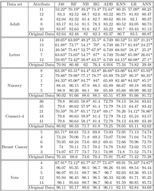
Some attributes will have a strong influence on the class; others will have a much weaker influence. To determine the strength, we found the five most influential attributes, based on the information gain ratio, for each data set. We then used 10-fold cross validation to calculate the performance of each learner, averaged over all change levels. Table 1 shows the different degrees of influence that the attributes have on the class. The ∗ in this table indicates that, using a paired t-test with an alpha of 0.05, the accuracy of the learner for corrupted data is significantly different from that for the original data. For the Adult, Vote and Connect-4 data sets, only one attribute has a substantial influence. For others, more attributes are influential: three attributes for Nursery, and all five for the Letter data set. For the Breast Cancer data set, only for the Decision Tree is there a statistically significant difference and then only for the first attribute. However,
as the percentage of positive samples is 30%, the accuracy of all algorithms on the original data is very close to 70%, that of the default classifier. Thus corrupting the attributes has little impact. We will drop this data set from further consideration.
For the Letter data set, AdaBoost uses a Decision Stump as its base classifier. The performance of a Decision Stump, on this data set, is close to that of de-fault classifier, so corrupting the attributes has little effect on its accuracy. The performance of the Neural network is also low, yet higher than that of AdaBoost and the change level does affect its performance significantly. The surprising point for connect-4 data set is that the first and the second most influential attributes do not have an impact on the accuracy that is statistically significant for any learner. However, the third most influential attribute does. Exactly why this occurs will need further investigation.
3.2 Ranking the Algorithms
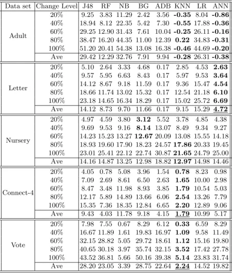
For each learner and each data set, we use the attributes that significantly affect the accuracy of the learner. First, we trained each learner using the original data set. We then tested it on data where the influence of the attributes has been decreased. We decreased the influence of each attribute using different change levels (20%, 40%, 60%, 80%, and 100%). The performance of each learner was averaged over all attributes for each change level. It should be noted that in Table 2 smaller is better, i.e. there is less change in performance. The best value in each row is in bold type. The average value of the best performing learner is underlined if it is significantly better than the value from the second best learner, using a paired t-test with a significance level of 0.05.
Let us go through the results of Table 2 by data set:
Adult The performances on clean and corrupted data are essentially indistin-guishable for Nearest Neighbor and the Neural Network. So the small nega-tive numbers are likely caused by random errors. So we conclude, on average, across all change levels, the Neural Network and Nearest Neighbor are the most robust learners.
Letter AdaBoost appears initially to be the most robust but, as explained ear-lier, the accuracy of AdaBoost on the original data set is very low and changing attributes has little effect. Excluding AdaBoost, Neural Network is the most robust at all levels. On average across all change levels, the Neural Network is the most robust learner and Random Forest is second.
Nursery Bagging is the most robust at lower change levels, while Nearest Neighbor is the best at higher levels. In addition, on average Nearest Neigh-bor is the most robust method but, using the t-test, it is not significantly different from the second best learner, Bagging.
Connect-4 Nearest Neighbor is the best learning algorithm at all change lev-els. On average across all levels, Nearest Neighbor is the best learner and AdaBoost the second best.
Vote Nearest Neighbor is the best model at all change levels. On average across all levels, Naive Bayes is the second best.
Table 1.Accuracy with decreasing the gain ratio
Data set Attribute J48 RF NB BG ADB KNN LR ANN
Adult 11 53.22* 70.19* 49.2* 74.4* 73.44* 80.35 57.09* 80.25 12 83.3 82.52 68.7 82.6 83.22 80.75 81.83 80.47 6 82.04 82.32 81.4 82.7 80.62 80.18 82.1 80.37 8 83.17 81.54 81.5 78.3 83.22 80.52 83.05 80.73 10 83.87 82.63 81.6 82.7 83.22 80.7 83.43 81.13 Original Data 82.64 82.48 82 82.3 83.37 80.7 83.5 80.87 Letter 14 49.05* 63.69* 49.2* 55.5* 6.749 60.52* 51.35* 21.21* 13 61.88* 73.7* 54.1* 70* 6.749 66.71* 61.84* 24.27* 11 49.56* 75.81* 52.7* 67.9* 6.749 68.94* 58.4* 25.2* 7 63.63* 73.03* 54.7* 67* 6.749 70.66* 65.98* 26.01* 12 59.95* 72.42* 50.8* 63.5* 6.749 64.15* 60.08* 27.1* Original Data 70.94 80.46 62 76.4 6.916 75.34 74.82 29.48 Nursery 8 63.38* 65.31* 64.4* 63.8* 46.68* 63.06* 64.85* 65.92* 2 79.86* 79.98* 77.1* 78.7* 65.89 79.23* 80.3* 80.35* 1 84.33* 85.06* 84.7* 84* 65.89 82.46* 84.92* 85.5* 7 88.41 90.15 87.9 88.5 65.89 86.67 89.18 89.92 5 88.9 90.26 88.1 88 65.89 85.68 89.99 90.32 Original Data 90.02 91.66 88.6 88.5 65.51 87.89 91.66 91.72 Connect-4 36 79.8 80.63 58.8* 81.4 72.79 78.13 58.34 83.61 35 79.8 80.62 57.9* 81.4 72.79 78.13 64.47 83.42 21 70.59* 76.3* 65.1* 72.6* 69.1* 76.26 54.12* 76.86* 18 79.8 80.63 59.8* 81.4 72.79 78.12 65.24 83.57 41 79.8 80.64 58.1* 81.4 72.79 78.13 64.89 83.49 Original Data 80.02 80.33 71.7 81.8 73.25 78.05 65.11 82.02 Breast Cancer 5 65.71* 68.61 72.3 69.8 73.93 72.95 71.13 74.74 4 73.24 70.06 71.8 69.2 73.07 73.94 71.04 74.72 6 70.95 68.24 73.6 69.2 69.41 72.66 70.96 72.79 9 74 70.11 73.7 70.2 74.78 73.82 72.02 75.57 3 74.07 67.77 73.7 72.1 74.98 74.8 71.52 75.74 Original Data 76.44 68.6 74.6 70.4 75.91 75.87 71.42 75.28 Vote 4 67.91* 72.12* 85.7* 67.7* 73.47* 89.91 78.33* 74.87* 3 96.07 95.35 90.5 96.7 96.26 91.04 88.54 94.44 5 96.07 95.51 89.7 96.7 96.7 92.03 83.36 95.13 12 95.94 96.45 90.1 96.5 96.33 92.06 91.71 95.25 14 96.1 95.64 89.7 96.7 96.6 91.59 90.85 95.72 Original Data 96.11 95.17 89.6 96.4 96.11 92.15 92.84 94.69
Table 2.The impact of change level on the difference in performance
Data set Change Level J48 RF NB BG ADB KNN LR ANN
Adult 20% 9.25 3.83 11.29 2.42 3.56 -0.35 8.04 -0.86 40% 18.94 8.12 22.35 5.42 7.30 -0.55 17.88 -0.36 60% 29.25 12.90 31.43 7.61 10.04 -0.25 26.11 -0.16 80% 38.47 16.20 44.35 11.00 12.39 0.22 34.83 -0.31 100% 51.20 20.41 54.38 13.08 16.38 -0.46 44.69 -0.20 Ave 29.42 12.29 32.76 7.91 9.94 -0.28 26.31 -0.38 Letter 20% 5.10 2.64 3.33 4.68 0.17 2.85 4.53 2.63 40% 9.57 5.95 6.63 8.43 0.17 5.97 9.53 3.64 60% 14.12 8.67 9.18 11.59 0.17 9.36 15.47 4.54 80% 18.66 11.74 13.02 15.32 0.17 12.54 21.18 6.10 100% 23.18 14.65 16.34 18.29 0.17 15.02 25.72 6.69 Ave 14.12 8.73 9.70 11.66 0.17 9.15 15.29 4.72 Nursery 20% 4.97 4.59 3.80 3.12 5.52 3.78 4.85 4.38 40% 9.69 9.53 9.16 8.14 13.07 8.49 9.34 9.27 60% 14.23 15.23 13.27 12.67 20.09 13.08 15.55 14.18 80% 18.93 19.60 17.90 18.23 24.57 17.86 20.33 19.45 100% 23.01 25.41 22.12 22.74 30.87 21.65 24.79 25.00 Ave 14.16 14.87 13.25 12.98 18.82 12.97 14.98 14.46 Connect-4 20% 4.05 0.78 5.08 3.96 1.54 0.78 8.23 0.98 40% 7.09 2.69 8.61 6.50 2.63 1.65 10.00 2.98 60% 8.47 3.48 11.98 8.93 3.85 1.79 10.54 5.03 80% 12.17 5.89 14.89 13.66 6.06 2.54 13.26 7.79 100% 15.35 7.36 18.35 12.84 6.65 2.20 12.89 9.06 Ave 9.43 4.03 11.78 9.18 4.15 1.79 10.99 5.17 Vote 20% 7.98 7.55 0.67 8.29 6.12 0.33 6.59 8.29 40% 16.67 11.89 1.61 19.83 16.97 1.09 9.58 11.49 60% 32.15 28.82 5.05 29.72 18.61 1.12 15.16 19.80 80% 40.65 30.18 3.97 35.74 32.15 3.52 17.42 27.78 100% 43.52 36.81 5.66 50.16 39.38 5.14 23.83 31.74 Ave 28.20 23.05 3.39 28.75 22.64 2.24 14.52 19.82
Not surprisingly perhaps, a t-test for a significant difference between the best and the second best classifier does not give us all the information we require. The results are further validated for statistical significance using a one way analysis of variance followed by what is termed a post-hoc analysis [?]. First, the learners are tested to see if the average difference in performance, on the original and changed data, of the 8 learners are equal, across the five change levels and the most significant attributes respectively. This is the null hypothesis in ANOVA; the alternative hypothesis is that at least one learner is different. The results of the ANOVA are given in Table 3 allow us to reject the null hypothesis, but it does not tell us how to rank the classifiers.
Table 3.ANOVA with their corresponding F-Value and P-Value
Adult Letter Nursery Connect-4 Vote
F-Value P-Value F-Value P-Value F-Value P-Value F-Value P-Value F-Value P-Value 72.3 <0.0001 32.46 <0.0001 2.6 0.012 11.42 <0.0001 25.86 <0.0001
To achieve this we use the post-hoc analysis. We apply the Fisher’s LSD test, with an individual error rate of 0.05. Table 4 provides the average values of each metric for each learner, as well as their significant ranks, the columns labeled Ave and R respectively in this table. Note that if two or more instances have the same letter, then their performances are not significantly different. Table 4 shows the overall impact of changing the influence of all significant attributes over all change levels. For the Adult data set, the Neural Network and Nearest Neighbor are the most robust learners; the ensemble learners Bagging, AdaBoost and Random Forest are next. For the Letter data set, although AdaBoost is the most robust learner the original accuracy of AdaBoost is close to the default classifier. Excluding AdaBoost from this data set, the Neural Network is the most robust and Random Forest, Nearest Neighbor, Naive Bayes, Bagging are the next. Nearest Neighbor, Random Forests, AdaBoost and the Neural Network are the most robust model, for the Connect-4 data set. Next are the Decision Tree, Bagging, Logistic Regression and Naive Bayes. For the Nursery data set, the post hoc test is not able to differentiate among the learners very well. The mean difference value of the learners is close to one another and the variance is high. In this data set all learners except AdaBoost are placed in the first level. For the Vote data set, the best learners are Nearest Neighbor and Naive Bayes, all other learners are in the next group.
From table 4, due to the high variance among learners in each data set, the post hoc tests does not differentiate among the learners very well. For the Adult data set, the post hoc test does not differentiate among the learners of the third group indicated by letter C. For the Letter data set, it also does not differentiate among the third group of the learners. This is repeated across the individual data sets.
Table 4.Overall impact of changing of gain ratio
Adult Letter Connect-4 Nursery Vote All data sets Alg Ave R Alg Ave R Alg Ave R Alg Ave R Alg Ave R Alg Ave R ANN -0.38 A ADB 0.17 A KNN 1.79 A KNN 12.97 A KNN 2.24 A KNN 5.18 A KNN -0.28 A ANN 4.72 B RF 4.03 A BG 12.98 A NB 3.39 A ANN 8.76 A BG 7.91 B RF 8.73 C ADB 4.15 A NB 13.25 A LR 14.52 B ADB 11.14 B ADB 9.94 B KNN 9.15 C ANN 5.17 A J48 14.16 A ANN 19.82 B RF 12.59 B RF 12.29 B NB 9.70 C J48 9.43 B ANN 14.46 A ADB 22.64 B BG 14.1 B LR 26.31 C BG 11.66 C BG 9.18 B RF 14.87 A RF 23.05 B NB 14.18 B J48 29.42 C J48 14.12 D LR 10.99 B LR 14.98 A J48 28.22 B LR 16.42 C NB 32.76 C LR 15.29 D NB 11.98 B ADB 18.82 B BG 28.75 B J48 19.07 D
To improve differentiation of the robustness of algorithms, in the last column of Table 4, we give the average values for each learner, and significant ranks, for all data sets combined. Here, Nearest Neighbor is the clear winner with the Neural Network in second place. Learners reliant on a smaller number of attributes such as Random Forests, AdaBoost and Bagging are next. AdaBoost is the best but, as it did poorly in terms of accuracy on a couple of original data sets, this robustness comes at some price. The Decision Tree comes firmly in last place. In general, our experimental results show that learners reliant on more attributes, tend to be more robust to the changes of the influence of some of them.
4
Discussion and Future Work
In this section, we discuss some hypotheses for why some learners are more robust to changing the influence of attributes than the others. These need verification and will be the subject of future work. We will also discuss other directions for future research.
For Artificial Neural Networks robustness to attribute changes is dependent on a decision surface using all attributes of the data simultaneously. Thus, the changing of one attribute of an instance is unlikely to cause that instance to be misclassified, unless the weight of that attribute is very much larger than that of others. Likewise for Nearest Neighbor all attributes are used to find the distance between two instances. If the influence of one attribute decreases, other attributes can still be predictive. For decision trees such as J48, where the complexity of the tree depends on the data set we use, often only a few attributes define the decision boundary. Thus, if the influence of one of these attributes on one particular instance on the class is changed, then that instance may well cross the decision boundary.
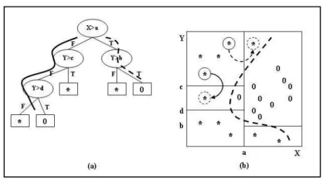
For example, Figure 1(a) is the decision tree and Figure 1(b) is the data and decision boundary formed by the tree (solid lines) and that formed by the Neural
Fig. 1.The impact of noise on decision tree and Artificial neural network
Network (dashed line). Note that x is the most significant attribute for decision tree. Now suppose that by changing the influence of this attribute,the instance at the top of the figure 1,moves in the x direction crossing the decision boundary for the tree. That instance will now travel down the right branch of the decision tree as shownby dashed linein Figure 1(a), classifying this instance incorrectly. This instance does not cross the decision boundary for the Neural Network. This is because this boundary uses both attributes and is much smoother. The same reasoning can be applied to instancecrosses the y=c boundary. in Figure 1 (b). If by changing the second most influential attribute (y) the instance crosses the boundary y=c. Then the leftsolidbranch on the tree classifies this instance as 0 but the Neural Network correctly classifies it.
Ensemble algorithms, as they consist of multiple classifiers, tend to rely on many though not all attributes. Where they differ, from each other, is primarily in the way the individual classifiers are constructed. Weremoved ”might”expect that Random Forests, by deliberately selecting classifiers based on different at-tributes, would be the most robust. That isremoved ”somewhat”supported by our experimental results in that it does well on a couple of data sets. It is, how-ever, beaten overall by AdaBoost, although the poor performance of AdaBoost on some original data sets removed ”may” account for much of this. Further experiments are needed to determine whether or not there is any real difference between ensemble algorithms in terms of robustness. If there is, we aim to find out what is at the root these differences. What is clear, however, is that they are generally better than the base classifier they use.
We had concerns that the statistical tests, which showed AdaBoost to be very robust, might be misleading due to its poor performance on some of the original data sets. So, we claim that for an algorithm to be considered robust it must not only have a small difference in performance, but also the performance on the original data set must be good, or at least competitive with other algorithms. As
future work, it would be worth exploring if a single metric might capture these two concerns. An alternative would be to plot points showing how they trade-off on a two-dimensional graph, similar to ROC curve or cost curves [9, 5]. Another concern with the experiments is that the measure we used, information gain ratio, is also used by the decision tree algorithm to chose the attributes at each branch. So, it may have a larger impact on the performance of decision trees than on that of other algorithms. We will therefore explore the effect of using different measures for selecting the most significant attributes in the future experiments. This can be quite easily realized within Weka as it has many attribute evaluators: Info Gain, Relief Attribute Evaluator, Principal Components, and OneR.
As other future work, the experiments will look at a greater range of al-gorithms. It would be worth exploring if there are other general characteristics, apart from the number of attributes used, that affect robustness. Another simple extension of current research is to include more data sets also using the whole size of datasets instead of just 10% of size we used in this work . Some of the data sets we chose only had one significant attribute. This property has been noticed before, simple classifiers often do well on UCI data sets [6]. It may be worth doing experiments on data sets with a wide spread in number of signifi-cant attributes, to see how this affects robustness. We will also experiment with changing the influence of a combination of attributes instead of one attribute at a time and with changing attributes in other ways.
We believe this paper has given some insight into what makes a classifier robust to changing environments. Nevertheless we have not explained by any means all the factors. We need to determine why Naive Bayes and Logistic Regression, which use all attributes, are not robust. Further experiments will be needed to expose the other differences between classifiers.
5
Conclusions
The objective of this study was to investigate the robustness of a variety of com-monly used learning algorithms to changing environments. The Neural Network and Nearest Neighbor are the most robust, learners reliant on smaller number of attributes such as Random Forest, AdaBoost and Bagging are located in the second place and finally the Decision Tree is in last place. In general, we conclude that learners reliant on more attributes tend to be more robust. This is clearly not the whole story, however, as Naive Bayes and Logistic Regression are not robust, future work will investigate this issue further.
Acknowledgments
We would like to thank the Natural Sciences and Engineering Research Council of Canada for the financial support that made this research possible.
References
1. R. Alaiz-Rodr´ıguez, A. Guerrero-Curieses, and J. Cid-Sueiro. Minimax regret clas-sifier for imprecise class distributions. Journal of Machine Learning Research, 8:103–130, 2007.
2. R. Alaiz-Rodr´ıguez and N. Japkowicz. Assessing the impact of changing environ-ments on classifier performance. In Proceedings of the 21st Canadian Conference
in Artificial Intelligence, pages 13–24, 2008.
3. Cathy Blake and Christopher Merz. UCI repository of machine learning databases. univ. of california at irvine. http://www.ics.uci.edu/~mlearn/MLRepository. html, 1998.
4. Chris Drummond. Discriminative vs. generative classifiers for cost sensitive learn-ing. In L. Lamontagne and M. Marchand, editors, Proceedings of the Nineteenth
Canadian Conference on Artificial Intelligence, LNAI 4013, pages 481–492, 2006. 5. Chris Drummond and Robert C. Holte. Cost curves: An improved method for
visualizing classifier performance. Machine Learning, 65(1):95–130, 2006.
6. Robert C. Holte. Very simple classification rules perform well on most commonly used datasets. Machine Learning, 11(1):63–91, 1993.
7. J. Huang, A.J. Smola, A.G retton, K.M. Borgwardt, and B. Sch¨olkopf. Correcting sample selection bias by unlabeled data. In B. Sch¨olkopf, J.Platt, and T.Hoffman, editors, Advances in Neural Information Processing Systems 19, pages 601–608. MIT Press, 2007.
8. F. Provost and T. Fawcett. Robust classification for imprecise environments.
Ma-chine Learning, 42:203–231, 2001.
9. Foster Provost, Tom Fawcett, and Ron Kohavi. The case against accuracy estima-tion for comparing inducestima-tion algorithms. In Proceedings of the Fifteenth
Interna-tional Conference on Machine Learning, pages 43–48, San Francisco, 1998. Morgan Kaufmann.
10. J. Ross. Quinlan. C4.5 Programs for Machine Learning. Morgan Kaufmann, San Mateo, California, 1993.
11. Joaquin Quionero-Candela, Masashi Sugiyama, Anton Schwaighofer, and Neil D. Lawrence. Dataset Shift in Machine Learning. The MIT Press, 2009.
12. P.D. Turney. Exploiting context when learning to classify. In Proceedings of the
European Conference on Machine Learning, pages 402–407, 1993.
13. P.D. Turney. The management of context-sensitive features: A review of strate-gies,. In Proceedings of the 13th International Conference on Machine Learning:
Workshop on Learning in Context-Sensitive Domains, pages 60–66, 1996. 14. G. Widmer and M. Kubat. Learning in the presence of concept drift and hidden
contexts. Machine Learning, 23:69–101, 1996.
15. Ian H. Witten and Eibe Frank. Data Mining: Practical machine learning tools and