An inconditionnally stable discontinuous Galerkin method for solving the 2D time-domain Maxwell equations on unstructured triangular meshes

(1)

HAL Id: hal-00178265

https://hal.archives-ouvertes.fr/hal-00178265

Submitted on 10 Oct 2007

HAL is a multi-disciplinary open access

archive for the deposit and dissemination of

sci-entific research documents, whether they are

pub-lished or not. The documents may come from

teaching and research institutions in France or

abroad, or from public or private research centers.

L’archive ouverte pluridisciplinaire HAL, est

destinée au dépôt et à la diffusion de documents

scientifiques de niveau recherche, publiés ou non,

émanant des établissements d’enseignement et de

recherche français ou étrangers, des laboratoires

publics ou privés.

method for solving the 2D time-domain Maxwell

equations on unstructured triangular meshes

Adrien Catella, Victorita Dolean, Stephane Lanteri

To cite this version:

Adrien Catella, Victorita Dolean, Stephane Lanteri. An inconditionnally stable discontinuous Galerkin

method for solving the 2D time-domain Maxwell equations on unstructured triangular meshes. IEEE

Transactions on Magnetics, Institute of Electrical and Electronics Engineers, 2008, 44(6).

�hal-00178265�

(2)

An unconditionally stable

discontinuous Galerkin method

for solving the 2D time-domain Maxwell equations

on unstructured triangular meshes

Adrien Catella, Victorita Dolean and St´ephane Lanteri

Abstract—Numerical methods for solving the time-domain Maxwell equations often rely on cartesian meshes and are variants of the finite difference time-domain (FDTD) method due to Yee [1]. In the recent years, there has been an increasing interest in discontinuous Galerkin time-domain (DGTD) methods dealing with unstructured meshes since the latter are particularly well adapted to the discretization of geometrical details that char-acterize applications of practical relevance. However, similarly to Yee’s finite difference time-domain method, existing DGTD methods generally rely on explicit time integration schemes and are therefore constrained by a stability condition that can be very restrictive on locally refined unstructured meshes. An implicit time integration scheme is a possible strategy to overcome this limitation. The present study aims at investigating such an implicit DGTD method for solving the 2D time-domain Maxwell equations on non-uniform triangular meshes.

Index Terms—time-domain Maxwell’s equations, discontinuous Galerkin method, implicit time integration, local refinement, unstructured mesh.

I. INTRODUCTION

I

N the numerical treatment of the time-domain Maxwell equations, finite difference time-domain (FDTD) methods based on Yee’s scheme [1] are still prominent because of their simplicity (a time explicit method defined on cartesian meshes) and their non-dissipative nature (they hold an energy conservation property which is an important ingredient in the numerical simulation of unsteady wave propagation problems). Unfortunately, when dealing with complex geometries, the FDTD method is not always the best choice since a local refinement of the grid, albeit possible through a subgrid-ding technique [2], has an adverse effect on accuracy and efficiency. In particular, local refinement can translate in a very restrictive time step in order to preserve the stability of the explicit leap-frog scheme used for time integration in the FDTD method. Finite element time-domain (FETD) methods based on unstructured meshes can easily deal with complex geometries however they induce heavy computations or require accurate and efficient lumping of mass matrices [3].

A. Catella and S. Lanteri are with INRIA, 06902 Sophia Antipolis, France (e-mail:{Adrien.Catella, Stephane.Lanteri}@inria.fr).

V. Dolean is with the Nice/Sophia Antipolis University, J.A. Dieudonn´e Mathematics Lab., UMR CNRS 6621, 06108 Nice, France (e-mail: Vic-torita.Dolean@unice.fr).

The authors gratefully acknowledge support from CEA/CESTA under grant No. 4600 118950.

Manuscript received June 24, 2007.

Finite volume time-domain (FVTD) methods on unstructured meshes also appeared as an alternative to FDTD methods, but they suffer from numerical diffusion resulting from the use of upwind schemes [4], and their extension to high-order accuracy is a tedious task. Discontinuous Galerkin time-domain (DGTD) methods can handle unstructured meshes and deal with discontinuous coefficients and solutions [5]. They can be seen as generalizations of the FVTD methods, where the finite element approximation is piecewise constant inside elements. The different achievements of the FVTD methods are now being extended in the context of DGTD methods which enjoy a renewed favor nowadays and are used in a wide variety of applications [6] as people rediscover the abilities of these methods to handle complicated geometries, media and meshes, to achieve a high order of accuracy by simply choosing suitable basis functions, to allow long-range time integrations and, last but not least, to remain highly parallelizable. However, DGTD methods suffer from the same limitation concerning the allowable time step on locally re-fined unstructured meshes. In this study, we investigate the applicability of an implicit time integration strategy in order to overcome the stability constraint which characterize explicit DGTD methods in the context of the numerical resolution of two-dimensional Maxwell’s equations on locally refined unstructured triangular meshes.

II. IMPLICITDGTDMETHOD

The starting point of this study is the explicit DGTD method presented in [5] for solving the time-domain Maxwell equa-tions on simplicial meshes. Beside a standard discontinuous Galerkin formulation, this method is based on two basic ingredients: a centered approximation for the calculation of numerical fluxes at inter-element boundaries, and an explicit leap-frog time integration scheme. The implicit DGTD method proposed here differs from its explicit counterpart in the time integration scheme which is now chosen to be a Crank-Nicolson scheme. We consider the two-dimensional Maxwell equations in the TMz polarization on a bounded domain Ω ⊂ R2 :        ²∂Ez ∂t − ∂Hy ∂x + ∂Hx ∂y = 0, µ∂Hx ∂t + ∂Ez ∂y = 0, and µ ∂Hy ∂t − ∂Ez ∂x = 0, (1)

(3)

with boundary conditionsn×E = 0 on Γmandn×E −

zn × (H × n) = n × Einc− zn × (Hinc× n) on Γa where

ΓaS Γm= ∂Ω, being z =pµ/ε the impedance. We assume

a partition Th of Ω into a set of triangles Ti and we seek for

approximate solutions to (1) in the finite dimensional space Vp(Th) := {v ∈ L2(Ω) : v|Ti ∈ Pp(Ti) , ∀Ti ∈ Th}, where

P_p_(T_i_{) denotes the space of nodal polynomials {ϕ}_ij_}d j=1 of

total degree at most p on the element Ti. The space Vp(Th)

has the dimensiond, the local number of degrees of freedom. Note that a function vhp ∈ Vp(Th) is discontinuous across

element interfaces. For two distinct triangles Ti and Tk in

Th, the intersection Ti∩ Tk is an (oriented) edge aik which

we will call interface, with oriented normal vector ~nik. For

the boundary interfaces, the indexk corresponds to a fictitious element outside the domain. Finally, we denote byVithe set of

indices of the elements neighboringTi. The DGTD-Ppmethod

at the heart of this study is based on a Crank-Nicolson time scheme and totally centered numerical fluxes at the interface between elements. Decomposing Hx,Hy andEz on element

Ti according to: Hx(., t n_{) =} d X j=1 Hn xijϕij, Ez(., t n_{) =} d X j=1 En zijϕij,

where x ∈ {x, y}. Using the notations En zi = (En zi1, . . . , E n zid) t and Hn xi = (H n xi1, . . . , H n xid) t_{, the implicit} DGTD-Pp method writes:                              ²iMi En+1zi − E n zi ∆t = −K x iH n+1 2 yi + K y iH n+1 2 xi + X k∈Vi ¡Gn+_x 12 ik − G n+1 2 yik ¢, µiMi Hn+1xi − H n xi ∆t = K y iE n+1 2 zi − X k∈Vi Fn+_y 12 ik , µiMi Hn+1yi − H n yi ∆t = −K x iE n+1 2 zi + X k∈Vi Fn+_x 12 ik ,

being Mi the local mass (symmetric positive definite) matrix,

and Kx

i the (skew-symmetric) stiffness matrix. The vector

quantities Fn+12

xik and G

n+1 2

xik are defined as:

Fn+12 xik = S x ikE n+1 2 zk , G n+1 2 xik = S x ikH n+1 2 xk , where Sx

ik is the d × d interface matrix on aik which verifies t_Sx

ik = −Sxki (if aik is an internal interface) and tSxik = Sxik

(if aikis a boundary interface). Moreover:

En+12 zk = En zk+ E n+1 zk 2 and H n+1 2 xk = Hn xk+ H n+1 xk 2 . In [7], we prove that the resulting implicit DGTD-Pp

method is non-dissipative (if Γa = ∅) and unconditionally

stable. This method requires the resolution of a sparse linear system at each time step but, for non-dispersive materials, the coefficient of this system are time independent, a feature that can be taken into account to minimize the additional computational overheadand. Thus, we have adopted here a multifrontal sparse matrix direct solver [8]. The sparse matrix characterizing the implicit DGTD-Pp method has a block

structure where the size of a block is 3np× 3np, np being

the number of degrees of freedom associated to a nodal polynomial basis of the space Pp i.enp= ((p + 1)(p + 2))/2.

This matrix is factored once for all before the time stepping loop. Then, each linear system inversion amounts to a forward and a backward solve using the triangular L and U factors.

III. NUMERICAL RESULTS

The numerical results presented here aim at comparing the explicit leap-frog based DGTD-Pp method and the implicit

Crank-Nicolson based DGTD-Pp method. Simulations are

performed on a personal workstation equipped with an AMD Opteron 2 GHz processor.

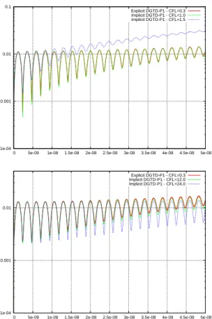
A. Eigenmode in a metallic cavity

The first test case that we consider is the propagation of an eigenmode in a unitary square cavity with perfectly conducting (PEC) walls. This test case allows a direct comparison with an exact solution. Here, it will also be used to demonstrate both the limitations in terms of accurarcy of the implicit DGTD-Pp

method if the underlying mesh is uniform (or quasi-uniform) and the potential gains in CPU times that one can expect in the case of a non-uniform mesh. For this purpose, we make use of two triangular meshes:

• a uniform mesh consisting of 1681 vertices and 3200 triangles. The non-dimensioned time step corresponding to CFL-P0=1 is(∆t)u= 0.017678 m (the physical time

step is defined by (∆t)u = (∆t)u/3.108 m/s). For the

interpolation orders p ≥ 1, the time step actually used is CFL-Pp× (∆t)u where CFL-Pp is the CFL number

associated to the DGTD-Pp method.

• a non-uniform mesh consisting of 1400 vertices and 2742

triangles. The ratio between the largest and smallest edges of this mesh is 178. In this case, the minimum and maximum values of the time step are respectively given by(∆t)m= 0.000434 m and (∆t)M = 0.070617 m. The

time step used in the simulations is CFL-Pp× (∆t)m.

For the explicit DGTD-Pp method, CFL-Pp ≤ 1 and the

actual value is dictated by stability issues while CFL-Pp can

be set to an arbitrarily large value for the implicit DGTD-P_p _{method but is constrained in practice by accuracy issues.} Here, we only report on results obtained using the explicite and implicit DGTD-P1 methods. On Fig. 1 we have represented

the time evolutions of the L2 error between the numerical and exact solutions. CPU times are given in Tab. I. Two main remarks can be made:

• although the implicit DGTD-Pp method is

uncondition-ally stable, the CFL (and thus the time step) must be selected in order to ensure that the resulting solution is not altered by an increased level of dispersion error.

• as expected, the overhead introduced by the resolution

of a linear system at each time step is minimized for large values of the CFL. Then the goal is to find a good compromise between the accuracy of the calculation and the required computational effort.

(4)

1e-04 0.001 0.01 0.1

0 5e-09 1e-08 1.5e-08 2e-08 2.5e-08 3e-08 3.5e-08 4e-08 4.5e-08 5e-08 Explicit DGTD-P1 - CFL=0.3 Implicit DGTD-P1 - CFL=1.0 Implicit DGTD-P1 - CFL=1.5 1e-04 0.001 0.01

0 5e-09 1e-08 1.5e-08 2e-08 2.5e-08 3e-08 3.5e-08 4e-08 4.5e-08 5e-08 Explicit DGTD-P1 - CFL=0.3 Implicit DGTD-P1 - CFL=12.0 Implicit DGTD-P1 - CFL=24.0

Fig. 1. Eigenmode in a PEC cavity. Time evolution of the L2

error. Comparison between explicit and implicit DGTD-P1methods. Uniform mesh

(top) and non-uniform mesh (bottom). TABLE I

EIGENMODE IN APECCAVITY: CPUTIMES. Uniform triangular mesh

Time integration Method CFL-Pp CPU time

Explicit DGTD-P1 0.3 15 sec

Implicit - 1.0 44 sec - - 1.5 30 sec

Non-uniform triangular mesh

Time integration Method CFL-Pp CPU time

Explicit DGTD-P1 0.3 443 sec

Implicit - 12.0 133 sec - - 24.0 67 sec

B. Scattering of a plane wave by a square

The second test case that we consider is the scattering of a plane wave by a perfectly conducting square of side length c = 0.25 m. The farfield boundary Γa where the first order

Silver-M¨uler absorbing condition is applied is defined as a square of side length c = 1.0 m. We make use of a non-uniform mesh consisting of 6018 vertices and 10792 triangles (see Fig. 2). The ratio between the largest and smallest edges is 357. In this case, the minimum and maximum values of the time step are respectively given by(∆t)m= 0.000286 m and

(∆t)M = 0.098589 m. As previously, the time step used in

the simulations is CFL-Pp× (∆t)m. Simulations have been

conducted for three frequencies of the incident plane wave, F=300 MHz, F=600 MHz and F=900 MHz and have been carried out for then periods. A discrete Fourier transform is

applied to the field components during the last period. Results are shown on Fig. 3 and 4 in terms of the x-wise 1D distribution for y = 0.25 m of the discrete Fourier transform (DFT) ofEz and for two frequencies (F=600 MHz

and F=900 MHz). For each configuration, we show the distri-bution of DFT(Ez) for the time explicit calculation which is

considered here as the reference solution, and two distributions of DFT(Ez) corresponding to time implicit calculations using

respectively the maximum allowable CFL yielding a solution that fit the reference one, and a larger CFL yielding a less accurate solution. Computing times are summarized in Tab. II. These results call for two main remarks:

• as expected, the maximum allowable CFL value decreases

when the frequency of the incident plane wave increases. Not surprisingly, despite the fact that the implicit DGTD-P_p_{method is unconditionally stable, the maximum} allow-able CFL value is deduced from physical considerations.

• as a result, for a given interpolation order, the gain in CPU time i.e the ratio of CPU time of the explicit DGTD-P_p _{calculation to the CPU time of the implicit} DGTD-P_p _{calculation, decreases when the frequency increases.} For instance, for p = 2 this ratio ranges from 7.5 for F=300 MHz to 3.0 for F=900 MHz. However, for a given frequency, this gain increases with the interpolation order: for F=900 MHz, this ratio is respectively equal to 3.0 for p = 2 and 5.5 for p = 3. X Y 0 0.5 1 0 0.1 0.2 0.3 0.4 0.5 0.6 0.7 0.8 0.9 1

Fig. 2. Scattering of a plane wave by a PEC square: triangular mesh TABLE II

SCATTERING OF A PLANE WAVE BY APECSQUARE: CPUTIMES. Frequency Time integration Method CFL-Pp CPU time

300 MHz Explicit DGTD-P1 0.3 1602 sec - Implicit - 15.0 370 sec - Explicit DGTD-P2 0.2 5677 sec - Implicit - 15.0 762 sec 600 MHz Explicit DGTD-P1 0.3 758 sec - Implicit - 7.0 383 sec - Explicit DGTD-P2 0.2 3074 sec - Implicit - 7.0 767 sec 900 MHz Explicit DGTD-P2 0.2 2191 sec - Implicit - 5.0 746 sec - Explicit DGTD-P3 0.1 8771 sec - Implicit - 5.0 1591 sec

(5)

IV. CONCLUSION AND FUTURE WORKS

We have studied here an implicit DGTD-Pp method for

solving the time-domain Maxwell equations on triangular meshes. The method is non-dissipative, second order accurate in time an p-th order accurate in space. As usual with time implicit schemes, this method requires the resolution of a sparse linear system at each time step. In the present case, the coefficients of the matrix are constant in time. Taking into ac-count this feature in the linear system solution strategy is a key ingredient for obtaining a computationally efficient method. For two-dimensional problems, a direct solver based on a LU factorization such as the one adopted in this study is generally considered as the optimal strategy, at least from the computing time point of view. Promising results have been obtained for time-domain electromagnetic wave propagation problems on locally refined unstructured meshes. Concerning future works, our main objective will be to adapt the implicit DGTD-Pp

method proposed here to the case of the three-dimensional time-domain Maxwell equations. In this context, it is clear that a global direct solver such as the multifrontal method adopted in this study will not be an acceptable option due to the large memory capacity required for the simulation of realistic three-dimensional problems, especially if the computational domain is discretized using unstructured tetrahedral meshes. In this context, parallel computing will be a mandatory path and although MUMPS [8] is a parallel sparse matrix solver, we plan to consider a Schwarz type domain decomposition method [9] as a mean to build an hybrid iterative/direct solver, and still benefit from the fact that the sparse matrix associated to a sub-domain problem can be factored once for all before the time stepping loop.

REFERENCES

[1] K. Yee, “Numerical solution of initial boundary value problems involving Maxwell’s equations in isotropic media,” IEEE Trans. Antennas and

Propagat., vol. 14, no. 3, pp. 302–307, 1966.

[2] S. Chaillou, J. Wiart, and W. Tabbara, “A subgridding scheme based on mesh nesting for the FDTD method,” Microwave and Optical Technology

Letters, vol. 22, no. 3, pp. 211–214, 1999.

[3] S. Pernet, X. Ferrieres, and G. Cohen, “High spatial order finite element method to solve Maxwell’s equations in time domain,” IEEE Trans. on

Antennas and Propagation, vol. 53, no. 9, pp. 2889–2899, 2005.

[4] J.-P. Cioni, L. Fezoui, L. Anne, and F. Poupaud, “A parallel FVTD Maxwell solver using 3D unstructured meshes,” in 13th Annual Review

of Progress in Applied Computational Electromagnetics, Monterey, CA,

USA, 1997, pp. 359–365.

[5] L. Fezoui, S. Lanteri, S. Lohrengel, and S. Piperno, “Convergence and stability of a discontinuous Galerkin time-domain method for the het-erogeneous Maxwell equations on unstructured meshes,” ESAIM: Math.

Model. and Numer. Anal., vol. 39, no. 6, pp. 1149–1176, 2006.

[6] B. Cockburn, G. Karniadakis, and C. Shu, Eds., Discontinuous Galerkin

methods. Theory, computation and applications, ser. Lecture Notes in

Computational Science and Engineering. Springer-Verlag, 2000, vol. 11. [7] A. Catella, V. Dolean, and S. Lanteri, “An implicit DGTD method for solving the two-dimensional Maxwell equations on unstructured triangular meshes,” INRIA, Tech. Rep. RR-6110, 2006. [Online]. Available: https://hal.inria.fr/inria-00126573

[8] P. Amestoy, I. Duff, and J.-Y. L’Excellent, “Multifrontal parallel dis-tributed symmetric and unsymmetric solvers,” Comput. Meth. App. Mech.

Engng., vol. 184, pp. 501–520, 2000.

[9] V. Dolean, L. Gerardo-Giorda, and M. Gander, “Optimized Schwarz methods for Maxwell equations,” 2006. [Online]. Available: https://hal.archives-ouvertes.fr/ccsd-00107263 -1.5 -1 -0.5 0 0.5 1 1.5 2 0 0.2 0.4 0.6 0.8 1 Explicit DGTD-P1 - CFL=0.3 Implicit DGTD-P1 - CFL=7.0 Implicit DGTD-P1 - CFL=8.0 -1.5 -1 -0.5 0 0.5 1 1.5 2 0 0.2 0.4 0.6 0.8 1 Explicit DGTD-P2 - CFL=0.2 Implicit DGTD-P2 - CFL=7.0 Implicit DGTD-P2 - CFL=8.0

Fig. 3. Scattering of a plane wave by a PEC square, F=600 MHz. 1D distribution of DFT(Ez), y = 0.75 m. DGTD-P1 method (top) and

DGTD-P2 method (bottom). -1.5 -1 -0.5 0 0.5 1 1.5 0 0.2 0.4 0.6 0.8 1 Explicit DGTD-P2 - CFL=0.2 Implicit DGTD-P2 - CFL=5.0 Implicit DGTD-P2 - CFL=6.0 -1.5 -1 -0.5 0 0.5 1 1.5 0 0.2 0.4 0.6 0.8 1 Explicit DGTD-P3 - CFL=0.1 Implicit DGTD-P3 - CFL=5.0 Implicit DGTD-P3 - CFL=6.0

Fig. 4. Scattering of a plane wave by a PEC square, F=900 MHz. 1D distribution of DFT(Ez), y = 0.75 m. DGTD-P2 method (top) and