HAL Id: hal-02283180
https://hal.archives-ouvertes.fr/hal-02283180
Submitted on 10 Sep 2019
HAL is a multi-disciplinary open access
archive for the deposit and dissemination of
sci-entific research documents, whether they are
pub-lished or not. The documents may come from
teaching and research institutions in France or
abroad, or from public or private research centers.
L’archive ouverte pluridisciplinaire HAL, est
destinée au dépôt et à la diffusion de documents
scientifiques de niveau recherche, publiés ou non,
émanant des établissements d’enseignement et de
recherche français ou étrangers, des laboratoires
publics ou privés.
Multi-level analysis of nutrient cycling within
agro-sylvo-pastoral landscapes in West Africa using an
agent-based model
Myriam Grillot, François Guerrin, Benoit Gaudou, Dominique Masse,
Jonathan Vayssières
To cite this version:
Myriam Grillot, François Guerrin, Benoit Gaudou, Dominique Masse, Jonathan Vayssières.
Multi-level analysis of nutrient cycling within agro-sylvo-pastoral landscapes in West Africa using an
agent-based model.
Environmental Modelling and Software, Elsevier, 2018, 107, pp.267-280.
Any correspondence concerning this service should be sent
to the repository administrator:
tech-oatao@listes-diff.inp-toulouse.fr
This is an author’s version published in:
http://oatao.univ-toulouse.fr/22464
To cite this version: Grillot, Myriam and Guerrin, François and
Gaudou, Benoit and Masse, Dominique and Vayssières, Jonathan
Multi-level analysis of nutrient cycling within agro-sylvo-pastoral landscapes
in West Africa using an agent-based model. (2018) Environmental
Modelling and Software, 107. 267-280. ISSN 1364-8152
Official URL
DOI :
https://doi.org/10.1016/j.envsoft.2018.05.003
Open Archive Toulouse Archive Ouverte
OATAO is an open access repository that collects the work of Toulouse
researchers and makes it freely available over the web where possible
Multi-level
analysis of nutrient cycling within agro-sylvo-pastoral landscapes in West
Africa
using an agent-based model
Myriam
Grillot
a,b,c,∗,
François Guerrin
d,
Benoit Gaudou
e,
Dominique Masse
f,g,
Jonathan Vayssières
a,b,c,∗∗ aCIRAD, UMR SELMET, Dakar, SenegalbSELMET, Univ Montpellier, CIRAD, INRA, Montpellier SupAgro, Montpellier, France c
Dp PPZS, Pastoral Systems and Dry Lands –Institut de recherche sénégalais Hann, BP2057, Dakar, Senegal dINRA, UMR SELMET, F-34398, Montpellier, France
eIRIT CNRS, Université de Toulouse, F-31062, Toulouse, France fIRD, UMR Eco&Sols, F-34060, Montpellier, France
g
LMI IESOL, Centre ISRA IRD Bel Air, BP1386, Dakar, Senegal
Keywords:
Biomass flows Crop-livestock integration Multi-agent system Multi-level modeling Nutrient spatial transfers Soil fertility management
A B S T R A C T
Livestock-driven nutrient flows are the main sources of soil and crop fertilization in West African agro-sylvo-pastoral landscapes. They result from nutrient recycling between farm activities and the spatial transfer of nutrients within the landscape. “Extensive” systems, based on livestock mobility are tending to be replaced by more “intensive” systems based on in-barn livestock fattening. We built an agent-based model to compare these systems in terms of nitrogen cycling at land plot, herd, household and village levels. Model evaluation, based on field-data from two real contrasted villages, showed that the model satisfactorily reproduces the differences between an “extensive” and an “intensive” system with key parameters such as variability among households and soil fertility gradients. Simulations highlighted bottlenecks along the nitrogen (N) cycle like accumulation of N in manure heaps and housing areas, reducing N recycling efficiency, especially in “intensive” systems. The model can be further used to explore improved agro-sylvo-pastoral landscapes.
1. Introduction
Crop-livestock systems encompass a variety of systems that take advantage of positive interactions between crop and livestock activities. These interactions can be materialized by different types of flows: biomass, nutrient, energy or cash flows. In West Africa, crop-livestock systems dominate rural areas (Herrero et al., 2010). With limited access to inputs, these “extensive” systems are typically agro-sylvo-pastoral systems (Powell et al., 2004). Biomass is recycled between crops, trees and livestock; e.g. crop residues and woody products are used to feed livestock and, conversely, livestock excreta (dung and urine) are key fertilizers for crops (Blanchard et al., 2013). Consequently, these sys-tems are characterized by high nutrient recycling rates between farming activities (Rufino et al., 2009). The systems are traditionally based on livestock mobility, free-grazing and night corralling practices, which have two major implications for the management of rural vil-lages in which they are implemented.
The first implication of these practices is strong interactions Software availability
Software name TERROIR model (version 1.3)
Developer contact address Myriam Grillot,myriam.grillot@ gmail.com
Year first available 2017
Hardware required Any recent PC with 200 MB of disk space and a minimum of 4 Gb of RAM, 32 or 64 bits for Windows & Linux, and 64 bits for MacOS X
Software required GAMA platform, version 1.7 ( http://gama-platform.org/)
Availability on open ABM (https://www.comses.net/codebases/ 5608/releases/1.3.0/)
Cost free for non-commercial use
∗Corresponding author. CIRAD, UMR SELMET, Dakar, Senegal. ∗∗Corresponding author. CIRAD, UMR SELMET, Dakar, Senegal.
E-mail addresses:myriam.grillot@gmail.com(M. Grillot),jonathan.vayssieres@cirad.fr(J. Vayssières).
models, which represent interactions between individuals (e.g. agents representing farms, herds, etc.) and their dynamics in a given landscape (Bousquet and Le Page, 2004;Ferber, 1995). Some agent-based models (ABM) were built to study crop-livestock systems, particularly through the simulation of biomass, nutrient or carbon flows. Each model has particular advantages: CaTMAS focuses on the role of fallow in the return of organic matter to the soil (Belem et al., 2011); PALM focuses on labor and economic flows (Matthews, 2006); SABLE and AMBAWA focus on the different uses of crop residues as a key biomass (Baudron et al., 2015; Diarisso et al., 2015). However, due to their reduced scopes, these models do not fully represent the biomass and nutrient cycles. In addition, night corralling, a key practice that determines nutrient spatial transfers in West African sustems, is not taken into account in AMBAWA, CaTMAS and PALM. In SABLE, night corralling is implemented, but the corresponding spatial transfers are not re-presented. Consequently, existing ABMs do not combine representa-tions of (i) interacrepresenta-tions between crop and livestock activities, (ii) live-stock-driven interactions between households and (iii) nutrient spatial transfers; whereas there is a need to take these processes into account to analyze the nutrient cycle in agro-sylvo-pastoral landscapes.
For these reasons, we built the TERROIR computer model — TERRoir level Organic matter Interactions and Recycling model — to assess soil fertility management and the nutrient recycling effi-ciency of agro-sylvo-pastoral landscapes. It is a spatially-explicit ABM that integrates nutrient cycling at different organizational levels (land plot, herd, household and village). The version of the model described here focuses on nitrogen (N) as a key limiting resource for both plant and animal production in West African agro-ecosystems (Schlecht et al., 2006).
The next section (Section2) describes the architecture and Section3
explains the implementation of the TERROIR model. Section4discusses the advantages and limits of the model. Model implementation com-pares two ‘real’ villages located in central Senegal that correspond to an “extensive” and an “intensive” system, exhibit contrasted landscape structures, crop rotations, and livestock and manure management practices. In this paper, particular attention is paid to how the in-formation generated at the different organizational levels in the model effectively represent N flows within the system as a whole.
2. Description of the model
The conceptual model is described according to the Overview Design concepts and Details protocol (ODD) (Grimm et al., 2013). It has been slightly adjusted to highlight the specificities of the model. To keep the paper as short as possible, further details and the full de-scriptions of the sub-models are provided in the Supplementary Mate-rial.
2.1. Overview 2.1.1. Purpose
The TERROIR model represents the management of a typical West African agro-sylvo-pastoral landscape in space and over time. It focuses on the processes that create biomass flows. These flows are converted into N, which is then used to assess soil fertility management.
The purpose of the model is to provide realistic estimations of the structure of N flows at different levels: land plot and herd, household and village. It is not intended to predict long term agro-ecosystem dy-namics but rather to compare different agro-ecosystems, depending on input parameters concerning the structure of the landscape (proportion of land units, §2.1.2.1) and crop-livestock systems diversity (linked to a typology of households, §2.1.2.2).
Two system levels are analyzed: the whole village, and the house-holds that make up the village. Use of the household level as the main determinant for decision-making enables simulation of heterogeneous behaviors and emerging patterns at the village level.
between households (in West Africa, the term ‘household’ is equiva-lent to ‘farm’) through livestock-driven biomass flows. Households with few livestock and large crop areas are biomass and nutrient providers, through crop residues, to households with more animals per cropping area (Tittonell et al., 2015). Households coordinate to favor livestock mobility within the landscape; to this end, they manage common grazing areas (e.g. rangelands) and organize livestock corridors con-necting rangelands and croplands (Dugué, 1998). Nutrients are dis-seminated throughout the landscape thanks to animal excreta.
The second implication is livestock-driven nutrient spatial trans-fers between land units within the village landscape (Hiernaux et al., 1997). Land units are defined as homogeneous parts of the village in terms of land use, management practices and biophysical processes (Zonneveld, 1989). In West Africa, village landscapes are classically structured in four concentric rings, corresponding to four land units (Manlay et al., 2004a; Ramisch, 2005). Starting from the center and moving toward the periphery, they comprise: (i) the “housing area”, where the homesteads are located; (ii) “home fields”, close to the homesteads, where the organic matter is concentrated in order to insure food security through the production of staple foods; (iii) “bush fields”, where cash crops are usually grown and fallow is organized for live-stock corralling and grazing during the cropping season; (iv) “range-lands”, forming the outermost ring of the village area, often corre-sponding to less fertile areas. Most of the year (except during the wet season), livestock graze in croplands and rangelands during the day and excrete in the home fields during night corralling. These practices drive nutrient spatial transfers from peripheral land units (rangelands and bush-fields) to core land units (home fields), resulting in a gradient of increasing soil fertility from the periphery to the center of the village (Manlay et al., 2004b; Tittonell et al., 2007b).
Due to high demographic growth in West Africa, the demand for crop and livestock products is rapidly increasing, leading to the ex-pansion of croplands onto rangelands, thereby constraining livestock mobility, see for instance in Burkina Faso (Vall et al., 2006). Conse-quently, the number of livestock and corresponding organic matter production are decreasing with a serious risk of soil fertility and crop productivity decline, as already pointed out by Pieri (1989),Lericollais (1999) and more recently by Agegnehu and Amede (2017). Two stra-tegies to maintain livestock activities are commonly observed. First, there are traditional “extensive” villages with organized fallows to isolate free-grazing livestock from crops. Second, there are “intensive” villages that are tending to abandon free grazing and changing to in-barn livestock fattening, which involves the purchase of large quantities of feed concentrate for animal fattening (Sow et al., 2004). Intensive systems mobilize more resources per hectare than the extensive sys-tems. These two situations also differ in terms of nutrient imports and in their management of organic matter; e.g. in the extensive system, ex-creta are directly deposited on the field by the animals, but are man-aged by humans as solid manure in the intensive system. This paper addresses the following questions: what are the differences between the two systems in terms of nutrient cycle organization? And, in both sys-tems, what are the bottlenecks that occur along the nutrient cycles and affect nutrient recycling efficiency and soil fertility?
Stock-flow simulation models are useful tools to analyze crop-live-stock systems, including agro-sylvo-pastoral systems. These models describe interactions between the system components to describe system functioning and performance, generally at farm level (Thornton and Herrero, 2001); see for instance farm representations through biomass flows by GANESH in Madagascar (Naudin et al., 2015), or through nutrient flows by NUANCES-FARMSIM in East Africa (van Wijk et al., 2009) or by SIMFLEX in Burkina Faso (Sempore et al., 2015). Farm simulation models are also used to analyze flows at the village level based on extrapolations from simulations made at the farm level (Andrieu et al., 2015; Rufino et al., 2011). However these models do not account for interactions between farms and the spatial organization of the villages. These two limits can be overcome using multi-agent
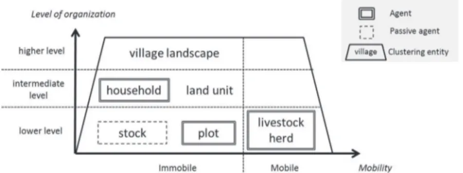
i) the lower level, which includes the livestock herds, biomass stocks and land plots;
ii) the intermediate level includes households, which make tactical and/or operational decisions that impact agents on the lower level (Cerf and Sébillotte, 1997;Fountas et al., 2006) and land units, which enables to group land plot according to their location; iii) the upper level, which corresponds to the whole village and where
the main emerging phenomena resulting from the dynamic inter-actions between lower level entities (e.g. households) are observed. Entities are static in space (immobile), except livestock herds that have the ability to move between land plots depending on their man-agement (determined by the households). Livestock mobility, places of feeding and excretion, as well as possible competition for local re-sources play a major role in the determinism of flows between land plots and hence, between land units.
2.1.2.1. Land plot. Like the real agro-sylvo-pastoral landscape in West Africa, the modelled village landscape is divided into four land units (moving from the center to the periphery: housing area, home fields, bush fields and rangelands). The total village area and landscape structure (defined in the model as the proportion of each land unit
within the village) are input parameters set by the user.
The model represents space as a 2D grid of square cells. Each cell (i.e. one land plot) has a fixed area of 0.25 ha, which is used as the smallest area managed by households. This area corresponds to the average size of the corrals used for night-time livestock enclosure (Achard and Banoin, 2003). At initialization, the land unit of each land plot is set according to its distance to the center of the village and the required proportion of each land unit in the village.
Land plots are grouped in two sub-classes: housingPlot and agriculturalPlot (Fig. 1). Housing plots are plots in which the house-holds live; agricultural plots include any plot that can be covered by vegetation other than trees, where most of the farming activities take place and livestock herds can wander freely. Agricultural plots belong to either the home fields, bush fields or rangelands land units. They can either be private assets managed by a household or a common resource of the village that can be used by all households (e.g. land plots in the rangelands).
Each land plot can hold trees, which are not represented as in-dividuals but as groups depending on whether they were pruned or not in the current year. In addition to tree products (leaves and wood), two types of biomass are produced on agricultural plots: natural vegetation (mostly grass) or crops (cereals, legumes). The type of biomass pro-duced depends on the use of the plot, which is based on the plot cropping plan. Cropping plans determine land use rotation (e.g. cereal, legume, fallow) on the plot over the years. The plans are decided on by the plot owner (i.e. a household agent) and can be adjusted to produce larger or smaller quantities of cereals, depending on the household's needs of staple food. Plots with no owner have a fixed land use: they grow natural vegetation.
2.1.2.2. Household. Households are the key agents in the model. A household is defined as a group of people who eat together (nuclear and/or extended family). Each household is located on a housing plot and belongs to a type that determines its parameters and decision scheme. A typology is used here to represent diverse resource endowment and crop and livestock practices. It is based on the one built byBalandier (2017)in central Senegal. Similar typologies have been developed in Burkina Faso (Vall et al., 2006). All households have
Fig. 1. Class diagram of the TERROIR model and its agent parameters.
2.1.2. Entities and organizational levels
In agro-sylvo-pastoral landscapes, the main acting and interacting entities are households and livestock herds. They interact with land plots, the smallest spatial entity in the model (used for either agri-cultural or housing purposes; not to be confused with land units, which are land plot categories). Households, livestock herds and land plots are represented as agents in the model, as are biomass stocks (food, feed and fuel). Stocks are considered as passive agents as they are op-erated by the households who own them; stocks do not make decisions but can be subject to internal biophysical processes (e.g. N losses). They are shown with their main attributes in Fig. 1, in the UML class diagram — Unified Modeling Language, see Bommel and Müller (2007) for more information on UML.
Three levels of organization are represented in the model, as shown in Fig. 2:
crop and livestock activities, whose intensity of practice vary according to the type of household. There are four types of households: crop-subsistence households (CS), livestock-crop-subsistence household (LS), crop-market (CM) and livestock-market (LM) oriented households.
Subsistence-oriented households (CS and LS), are low resource-en-dowment households that mainly aim to provide food for their family, in contrast to market-oriented households that aim to produce surpluses for agricultural markets (CM and LM) (Appendix A). Regarding live-stock management, subsistence-oriented households mainly practice free-grazing on wide areas and their feeding system is based on local forage resources; in contrast market-oriented households mainly prac-tice in-barn fattening and import feed concentrate. Subsistence-oriented households also use fewer inputs per hectare for their crops than market-oriented households and practice triennial rotations that in-clude fallow. For these reasons, subsistence-oriented households may be termed “extensive”, whereas market-oriented households may ba called “intensive”. In addition, crop-oriented households contrast with livestock-oriented households, depending on the main activity on which they rely.
The needs of households for food and fuel (wood and dung) depend
on the number of their members (set fixed during a simulation and fulfilled with weekly processes).
2.1.2.3. Livestock herd. Livestock is modelled as herd agents. Eash herd is defined as a group of animals of the same species that belong to the same owner (i.e. a household) and share the same type of management. The number of animals in a herd is measured in Tropical Livestock Units (TLU) used as a common unit. A TLU is equivalent to an animal of 250 kg live weight (1 adult zebu male = 1 TLU). Three livestock species are differentiated: bovine, small ruminant and equine. There are also three types of livestock systems in the model: free-grazing ruminants, in-barn ruminants, draft animals. Livestock herd agents are located on a land plot and, when in a free-grazing system, have the ability to move across the landscape and be located on any agricultural plot.
Free grazing is an extensive livestock system in which livestock herds are used to fertilize agricultural plots with excreta produced while grazing, and are kept in corrals at night. In-barn is an intensive livestock system that targets external markets. The in-barn system aims at fattening the animals for a fixed time period until they are sold. In-barn livestock herds are kept on the same housing plot as the household
Fig. 2. The six entities of the model, sorted according to their organizational level and their mobility.
An example is the use of stored food products: if stocks are emptied, then households proceed with imports, else they use their stock (see §2.2.5). If the cropping season has not been good enough (insufficient rainfall) to fulfill household food needs, the stocks will be used up faster than in better farming years and this will lead to more imports. Similarly for livestock, a bad cropping season produces fewer crop residues and consequently leads to greater use of natural resources, such as tree forage to meet feed needs.
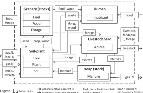
Actions within the systems create a network of interactions in the form of biomass flows (in kg of dry matter), occurring over time and in space between the system compartments. In the context of West African agro-sylvo-pastoral systems, we designed two conceptual stock-flow models to synthesize the simulated flows (Appendix B). The first model focuses on interactions among the farming activities of the households that make up the village. Its compartments are soil-plant, livestock herd, human (group of individuals living in a household), granary (food, forage and fuel stocks) and heap (manure stock). The human and granary related activities are included in the farm activities as home consumption is high in the systems studied here. The same conceptual representation has already been used to analyze crop-livestock inter-actions in similar systems (Alvarez et al., 2014;Rufino et al., 2006;
Stark et al., 2016). The second model focuses on flows circulating between the land units. The model compartments are housing areas, home fields, bush fields, rangelands. This spatial representation of system flows is used to analyze the spatial heterogeneity and gradients of soil fertility observed in similar systems (see Introduction).
Characterization of each biomass flow enables the two models to be intertwined; each biomass flow has (i) a farming activity of origin and one of destination (Appendix B1) and, (ii) a land unit of origin and one of destination (Appendix B2). For instance, during manure spreading, there is a flow of manure from the heap to the soil-plant compartment and from the housing area (where the heap is located) to home fields or bush fields, depending on the location of the plot.
2.2.1.2. Biophysical sub-models. In the model, biophysical processes are simple empirical sub-models. Crop and grass yields are computed annually, based on annual rainfall (in mm/year) and the quantity of N available. The model uses a water-limited yield curve and a fertilization coefficient based on available N (Sup. Mat. §4.2.2). The equation was determined with a mechanistic model, CELSIUS (Cereal and Legume crops Simulator Under changing Sahelian environment) (Affholder et al., 2012;Ricome et al., 2017). The quantity of available N depends on the quantity of mineral fertilizer and organic matter applied to the crops for the last three years. Not all the organic N applied is available right away, as part of N availability comes from a so-called “residual effect” of organic fertilization, due to the delayed process of organic N mineralization (Freschet et al., 2008). As crop and grass models are not dynamic, there is no impact of the exact date of the nutrient availability on yield computation. Consequently, mineral fertilization is annual and mineralization and losses are calculated annually. Weeds grow along with crops but do not impact the crop yields and are used green to feed in-barn livestock. Weed production is based on the average weed biomass measured in cultivated fields by
Achard and Banoin (2003)in Niger.
Each day, livestock herds ingest forage, feed concentrate and ex-crete dung and urine. The ingested quantity is limited by the ingestion capacity of the herd, which depends on the number of animals and species in the herd and the digestibility of the forage and feed con-centrate (Sup. Mat. §5.4.2). Fattening livestock ingest more biomass than free-grazing livestock, in terms of quantity of dry matter, as these animals are fed with concentrates, which are more digestible.
The feed intake changes over the course of the year, depending on the type of resource and period of availability, e.g. immediately after harvest, free-grazing livestock ingest more crop residues; during the wet season, fresh grass are distributed to in-barn livestock instead of hay, etc. (Chirat et al., 2014). Quantities also vary. Households increase the owner's home, which they only leave when they are sold. In-barn herds
are fed with forage and feed concentrate purchased on the external market. Animal feed requirements are higher in the in-barn system than in the free-grazing system. Draft livestock systems involve horses, in contrast to the two other systems that involve bovine and small rumi-nant herds. The management of herds of draft horses is similar to in-barn herds in terms of location and feed requirements. The objective is to maintain the animals in good condition for daily operations (carrying loads, especially manure, plowing, etc.).
Livestock herd variables are mainly related to feed consumption. All livestock agents have forage and feed concentrate requirements that vary depending on the livestock system and species concerned. Forage needs are divided into two types: need for low quality forage (cereal straw) versus need for high quality forage (legume hay, fresh weeds). 2.1.2.4. Household stocks. Stocks are located on a land plot depending on the type of biomass they store (e.g. at home in the granary for cereal cobs and on the closest agricultural plot for straw). There are two kinds of stocks: stocks for home consumption, i.e. food for the households (dry cereals and legumes), fuel for cooking (wood) and forage for livestock herds; and fertilizer heaps that store the manure (a mixture of excreta and refused animal feed) produced by the livestock herds located on housing plots (i.e. in-barn or draft livestock herds). Kitchen waste is not stored but directly spread on the fields located closest to home. Each household agent owns one stock per type of storable biomass.
Each stock is considered to be of unlimited capacity and includes the stock for daily use, which changes depending on the household's con-sumption; and surplus stock, which can theoretically be sold without causing any shortage for the household (§2.2.3).
2.1.3. Process overview and scheduling
The general sequence of actions in the model simulates one year in an agro-sylvo-pastoral landscape (Fig. 3). The beginning of the simu-lated year is based on the cropping season calendar: it begins the month of the first significant rainfall event and ends one year later. The model proceeds in daily steps; however some processes are abstracted on a weekly basis (i.e. updated every 7 time steps) and others on an annual basis (as a year is 12 months counting 30 days, these processes are updated every 360 time steps).
Before using the model for simulations analysis, we ran simulations over 30 years, under the hypothesis of no change in household popu-lation or in the landscape. We observed that convergence of simupopu-lation outputs was reached after only 5 years. In addition, we explored dif-ferent values of the number of replications and observed that simula-tions had to be repeated 8 times to overcome model stochasticity, i.e. to stabilize the variability within simulation outputs of the 5th year. Thus, in the model implementation and evaluation, we simulated the model over 5 years and ran 8 replications for each set of parameter values. Only the 5th year of each replication was retained and global simula-tion results are the average of the values for the 5th year of the 8 re-plications.
2.2. Design concepts 2.2.1. Basic principles
2.2.1.1. Household actions. In the model, daily household actions are performed based on the local interactions between households, livestock herds and their environment (Guerrin, 2009; Vayssières et al., 2007). The model used general guide rules, such as priority fertilization of home fields, livestock paddocking on the owner's plot, etc. Quantities are determined according to adjustable thresholds, e.g. family needs for the amount of land under millet, livestock needs for forage storage. The rules and thresholds are based on previous studies (Audouin et al., 2015; Lericollais, 1999). The household decision process is represented as a decision tree with if-then-else conditions.
the same village social network. Households prioritize exchanges with those with the highest stock surpluses.
Households also interact with each other through livestock. In a free-grazing management framework, herds interact with the plot in which they graze by taking up plant biomass and fertilizing it with their excreta. Herds may graze and excrete on plots owned by different owners, thus generating interactions between the household system and the plot system.
2.2.6. Observation
The model computes animal and plant production as a result of biological processes impacted by respectively animal feeding and soil fertilization, which both result from the actions of households and li-vestock herds. Yields can be observed in simulation outputs at the plot, household, land unit or village landscape levels. Herd demography and stock levels are monitored at the lower level of organization, i.e. at herd and stock level respectively.
The main observations are the biomass flows created by household and livestock actions and by the biophysical processes. These biomass flows (expressed in kg of dry matter per month) are converted into N flows (in kgN per month).
The model distinguishes two types of flows: (i) ‘actionable’ flows stemming from human actions, e.g. harvesting crops, feeding animals, spreading manure; (ii) ‘biophysical’ flows, mainly determined by nat-ural causes, e.g. N atmospheric deposition, fixation by legumes, leaching, run-off and gaseous emissions.
Biomass flows are represented at household and village landscape levels. The major difference between the two levels concerns interac-tions between households: biomass flows between two households are considered as external flows for both households, while at village landscape level they are considered as internal. Spatially, rangelands are not included at the household level while at the village landscape level the whole village area is taken into account, and consequently includes rangelands, which are common-pool resources.
In this paper, in order to fit model simulation outputs with available field data (based on village surveys), only actionable flows are used to calculate system assessment indicators (Rufino et al., 2009;Stark et al., 2016). We calculate (i) partial N balance (= input N – output N) to assess soil fertility maintenance (Schlecht and Hiernaux, 2004), as op-posed to full N balance that includes biophysical flows; (ii) N throughput (= sum of circulating N flows in the system) to assess the level of intensification of the system; and (iii) N recycling efficiency (= output N/input N) to identify bottlenecks in the N cycle (Rufino et al., 2006).
3. Model simulations
In this section we demonstrate the usefulness of the model to si-mulate and compare two contrasted agro-sylvo-pastoral landscapes. The model is coded with Gama (v1.7), a multi-agent simulation and spatially explicit modeling platform (Grignard et al., 2013;Taillandier et al., 2014).
3.1. Simulating two contrasted villages
Two villages located in the Senegalese groundnut basin (in central Senegal) were surveyed extensively in 2013 byAudouin (2014)and
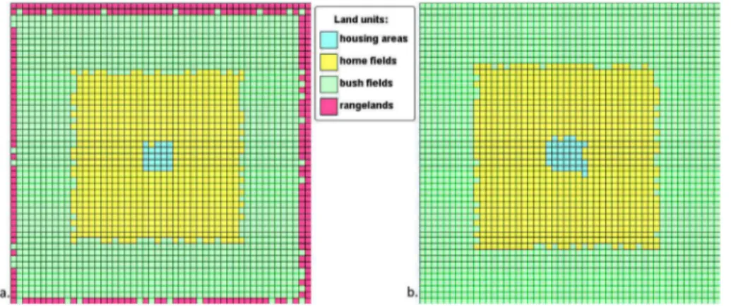
Odru (2013).Audouin et al. (2015)showed that the two villages are contrasted. The first village (Vext) was described as an “extensive” system with the dominance of subsistence-oriented households, based on free-grazing livestock. The second village (Vint) was described as an “intensive” system with the dominance of market-oriented households, with in-barn livestock fattening. The two village landscape structures are very different: in Vext, rangelands facilitate livestock mobility within the village, while in Vint there are no rangelands (Fig. 4). In addition, Vext fallows are collectively organized in order to isolate free-quantity of highly digestible forage (hay) and feed concentrate given to
livestock a few weeks before they are sold to produce fatter animals. Draft animals require more forage when they are working (spreading manure, sowing, harvesting). The quantity of N excreted as urine de-pends on the excretion of dung, which, in turn, depends on the quantity of N ingested the previous day (Sup. Mat. §6.2). Excreta deposits are proportional to the time spent by the animals on the plot. For instance, free-grazing herds spend a given time in their corral at night (by de-fault, in the model, the herd stays on the plot for 10 h, leading to the deposition in the corral of 10/24ths of the herd's daily excreta). 2.2.2. Stochasticity
Stochasticity is mainly introduced at simulation initialization when land plots are attributed to households and land use is determined (one of the possible crop rotations, according to the type of household and plot land unit, §2.1.2.2). At the end of each cropping season, house-holds update land use in their land plots according to the crop rotation of each plot. Then, in order to maintain a predetermined proportion of land plots with cereals to guarantee food security, households replace a non-cereal land use (fallow, legume) by cereals.
2.2.3. Predictions
Households estimate their annual needs for each type of stored biomass and then determine the surpluses of each they might have (Sup. Mat. §5.3). For instance, at the end of the cropping season and after adjusting their cropping plan (§2.2.2), households can determine the quantity of seeds to save for the upcoming cropping season. 2.2.4. Sensing
In West Africa, some activities are decided collectively; e.g. begin-ning of cereal sowing, the dates when transhumant livestock can arrive in the village and should leave it (Audouin et al., 2015;Dongmo et al., 2010). In the model, information at the village level is fixed by the modeler (e.g. introducing rules such as “sowing starts one month before the first rain”). All information is public (i.e. any agent can access to it), which is quite realistic as the modelled system is relatively small (vil-lage). Hence, household agents are assumed to know the availability of all products in their village, i.e. the amount of any surplus of all stocks.
Household decisions are made based on what they know from their own livestock and agricultural plots. For instance, the previous yields of their agricultural plots enable them to calculate which plots require more or less fertilizer.
In the model, livestock herd agents in free-grazing systems include a herder; each herder evaluates biomass availability on agricultural plots and leads the herd around the village land. In this way, free-grazing livestock herds are modelled as cognitive agents, autonomous from their household for grazing and corralling activities.
2.2.5. Interactions
Households interact with the entities they manage: cropping activ-ities have a direct impact on agricultural plot production, livestock feeding influences the quantity of excreta produced by the herd, stocking and destocking biomass influences the levels of stocks. With the exception of a few interactions, such as changing the land use of a plot, most interactions result in biomass and N flows.
When a household needs a product that is out of stock, it imports it from other households, if possible, within the village. If a product is not available in the village (e.g. fish, feed concentrate) or is sold out (e.g. straw), households buy it on the external market. As long as a product is available in the village (i.e. as a surplus) households will get it from another household. We use the term “purchase” when dealing with the external market and “exchange” when dealing with interactions be-tween households (including both monetary and non-monetary trans-actions). Imports are assumed to be unlimited (i.e. market prices and availabilities are not taken into account), and any household agent is likely to interact with any other household agent as they all belong to
grazing livestock in the village during the cropping season, while in Vint, most of croplands are cultivated.
Simulations were run for the two villages using the model input parameters listed inTable 1.
Table 1. Landscape structures were based on the real land unit proportions observed in the two villages. The corresponding grids were built by the model concentrically around the central cell (§2.1.2.1) (Fig. 4).
3.2. Simulation results
This section compares simulation results (Sim) for Vext and Vint. Field data (FD) are listed inTable 2but are only used in §4.1 for model evaluation. The first sub-section mainly refers to the first conceptual stock-flow model: interactions between farming activities (Appendix B.1), while the second sub-section compares spatial heterogeneity within villages resulting from N spatial transfers, with reference to the second conceptual model: interactions between land units (Appendix B2).
3.2.1. Interactions between activities
At compartment level, the soil-plant compartment is the only compartment in deficit (i.e. with a negative N balance) in both villages, while the others tend to accumulate N (Table 2). In Vint, livestock produce more excreta than in Vext (+8.9 kgN/ha). Accumulation is particularly high in the heap compartment in Vint (+10.2 kgN/ha more than in Vext). Variability at compartment level is higher in Vint than in Vext, due to the diversity of household types (there are only
subsistence-oriented households in Vext while both subsistence and market-oriented households coexist in Vint).
At household level, N balances are on average twice higher in Vint than in Vext, whereas efficiencies are on average 1.5 times lower in Vint than in Vext (Table 2). Pairwise comparisons using the Z-test revealed significant differences between households in Vext and Vint for bal-ances (p = 0.0092) and efficiencies (p = 0.018). However, variability was high among the households in each village; standard deviations ranged from 1.0 to 3.3 times the mean values. This reveals major dis-parities among households. For instance, in Vext, the N balance was on average 6 times higher in livestock-subsistence-oriented (LS) house-holds than in crop-subsistence-oriented (CS) househouse-holds. As LS have more free-grazing livestock than CS, they benefit from N transfers driven by their own livestock from fields owned by CS (where their livestock can graze during the day) to their own fields (where their livestock excretes during night corralling). In Vint, livestock-market-oriented (LM) households have N balances about 15 and 5 times higher than CS and crop-market-oriented (CM) households, respectively.
At village landscape level, the same differences as at household level were simulated between Vext and Vint for N balances and N efficiency (Table 2). More flows circulate in Vint than in Vext; throughput reaches 126.0 kgN/ha in Vint versus 95.3 kgN/ha in Vext. Flow intensification in Vint corresponds to an increase in both plant and animal production and explains why more people and animals can live in Vint; human population density is about 5.5 times higher and livestock stocking rate about 2 times higher in Vint than in Vext (Appendix C). In both villages, the main N imports are feed concentrates, which account for 59% and 66% of total imports in Vext and Vint, respectively; the main N exports are groundnuts, which account for 88% and 53% of total exports in Vext and Vint, respectively. Livestock exports are high in Vint, they account for 46% of total N exports, but for only 3% in Vext. In total, Vint imports +19.9 kgN/ha more than Vext; particularly +4.0 kgN/ha of feed concentrates and +2.5 kgN/ha of mineral fertilizers; Vint also exports +5.2 kgN/ha more than Vext.
3.2.2. Spatial heterogeneity
Soil-plant compartments tend to have an N deficit (see negative N balances inTable 2); however, strong spatial heterogeneity of the plot level N balance is found in both villages. Home fields have on average positive balances, in contrast to bush fields and rangelands (Table 3); they receive 4 and 6 times more organic and mineral fertilizer than bush fields in Vext and Vint, respectively. In Vext, cereal yields are 15% higher in home fields than in bush fields; similarly, in Vint, yields are 24% higher in home fields than in bush fields (Appendix C). Results highlight high N balances in housing areas (Table 3). Housing areas accumulate N mainly in the form of manure (see positive balance of manure heaps inTable 2and N in housing areas inTable 3).
At landscape and household levels, there is a decreasing gradient of N balances from the core land units (housing areas and home fields) to peripheral land units (bush fields and rangelands) (see Table 3).
Table 1
Input parameters of the two simulated villages (Vext, Vint).
Input parameters(1) Unit Vext Vint Households types
Number of households household units 6.84 7.70 Crop-subsistence oriented households
(CS)
% total households 10.90 11.75 Livestock-subsistence oriented
households (LS)
% total households 14.10 15.0 Crop-market oriented households (CM) % total households 18.0 19.20 Livestock-market oriented households
(LM)
% total households 22.0 23.5 Landscape structure and rainfall
Village area Hectares 29.376 30.376 Housing area % village area 33.1 34.1 Home fields % village area 37.10 38.45 Bush fields % village area 41.74 42.54 Rangelands % village area 45.14 46.0 Annual rainfall mm/year 49.680 50.680
(1)
Based on field data collected for the year 2013, (Audouin, 2014; Odru, 2013).
Fig. 4. Example of spatial grids generated by the model: two village landscape representations char-acterized by different structures. a. Village domi-nated by cultivated areas but where rangelands still exists in the landscape (Vext). b. Village where the total agricultural area is cultivated, there are no rangelands, and a larger proportion of home fields (Vint) compared to the other village.
However, in terms of efficiency, the reverse is true, as the land units that receive less N (rangelands and bush fields) produce more per kg of N input (Table 3). Livestock-driven flows are high in both villages, as livestock intake and excreta represent 52% and 49% of the total cir-culating N flows in Vext and Vint, respectively. Livestock excreta ac-count for 63% (i.e. 11.9 kgN/ha/year) and 43% (i.e. 10.6 kgN/ha/year) of the N inputs to the soil-plant compartment in Vext and Vint, re-spectively. Household manure accounts for on average only 8% ± 2 and 9% ± 1 of the cropland area in Vext and Vint, respectively. Within the land units, heterogeneity is higher in home fields than in bush fields in Vext (see spatial distribution plot-level N balances inAppendix D). As generally observed in the study area (Audouin et al., 2015) fields are fertilized once every two to three years, due to limited access to organic inputs. As soil storage is not taken into account in the calculation of N balance, the balance is high in the year fertilizer is applied and low the following years. In Vint, heterogeneity is lower in housing areas and home fields than in Vext because there are more market-oriented households that can import more mineral fertilizers to fertilize plots
when they are not fertilized with manure. 4. Discussion
4.1. Model evaluation
Model evaluation is essential but not straightforward, particularly when models seek to represent complex hard-to-measure systems in which decision making and biophysical processes interact (Bousquet and Le Page, 2004). This section aims to evaluate model performances by comparing simulation results for the two villages with field data from the same two villages (Audouin et al., 2015;Balandier, 2017) for N partial balances and efficiencies at the three levels of organization (seeTable 2). To our knowledge, such model evaluation, combining several levels of organization, is new for farming systems in West Africa. Field data were gathered retrospectively for year 2013, for all biomass and N flows between farming activities. It was an extensive task that was not extended to flows between land units due to the high
Table 2
N partial balances and N recycling efficiencies in 2013 based on field and simulation data for an extensive village (Vext) and an intensive village (Vint) at village, household and compartment levels.
Organizational level Vext Vint
N partial balance (kgN/ha/year)* N recycling efficiency (Dmnl) N partial balance (kgN/ha/year)* N recycling efficiency (Dmnl)
FD Sim FD Sim FD Sim FD Sim
Higher level: village
Village 4.0 7.3 0.6 0.4 25.4 22.0 66.0.3 67.0.3
Intermediate level: households**
All households 14.6 ± 33.2 14.2 ± 15.2 0.9 ± 1.0 0.5 ± 0.1 37.6 ± 47.9 23.4 ± 31.6 82.0.5 ± 0.5 83.0.4 ± 0.1 CS*** NA 9.1 ± 1.1 NA 0.4 ± 0.1 NA 10.6 ± 1.6 NA 0.4 ± 0.1
LS*** NA 59.7 ± 2.8 NA 0.3 ± 0.0 – – – –
CM*** – – – – NA 53.4 ± 50.3 NA 0.4 ± 0.0
LM*** – – – – NA 156.2 ± 1.1 NA 0.3 ± 0.0
Lower level: compartments**
Human 9.2 ± 8.4 7.7 ± 0.4 0.5 ± 0.3 0.5 ± 0.0 12.6 ± 6.7 8.9 ± 2.8 0.2 ± 0.2 0.4 ± 0.0 Livestock herd 3.3 ± 1.8 3.5 ± 1.8 0.7 ± 0.2 0.2 ± 0.1 2.1 ± 12.4 0.2 ± 6.5 1.0 ± 0.2 1.1 ± 0.1 Heap (manure) 5.8 ± 6.9 6.5 ± 0.8 0.6 ± 0.6 0.3 ± 0.0 20.1 ± 27.6 16.7 2 ± 24.0 0.7 ± 1.9 0.2 ± 0.1 Soil-plant −5.1 ± 19.0 −14.3 ± 7.0 3.4 ± 3.2 1.8 ± 0.3 −9.8 ± 24.2 −13.5 ± 1.7 1.5 ± 1.1 1.6 ± 0.1 Granary −1.8 ± 19.4 10.9 ± 0.7 1.2 ± 0.9 0.6 ± 0.0 15.0 ± 41.1 11.1 ± 1.4 0.8 ± 0.9 0.6 ± 0.1
FD = field data; Sim = simulations; Dmnl = dimensionless; NA = not available; - = do not exist.
*at village level, per hectare of the village area; at household level, per hectare of the household cultivated area.
** mean ± standard deviation for the household population in each village; n = 84 households for Vext and n = 70 households for Vint. *** Household types: CS = crop-subsistence; LS = livestock-subsistence; CM = crop-market; LM = livestock-market.
Table 3
Simulated N partial balances and N recycling efficiencies in 2013 for an extensive village (Vext) and an intensive village (Vint) at village, household and com-partment levels.
Organizational level Vext Vint
N partial balance (kgN/ha/year)* N recycling efficiency (Dmnl) N partial balance (kgN/ha/year)* N recycling efficiency (Dmnl) Higher level: whole village landscape
Housing areas 1888.2 0.4 2128.2 0.3
Home fields 13.1 . 0.7 16.3 0.7
Bush fields −21.4 2.8 −23.0 3.5
Rangelands −23.1 3.6 −14.3 3.3
Medium level: individual households**
Housing areas 1137.6 ± 30.9 0.5 ± 0.0 1756.4 ± 341.4 0.5 ± 0.1 Home fields 19.4 ± 41.6 0.9 ± 0.2 26.3 ± 2.8 1.1 ± 0.2 Bush fields −21.8 ± 2.8 3.0 ± 1.2 212.−24.3 ± 2.2 5.2 ± 4.8
* at village level, per hectare of the land unit within the village; at household level, per hectare of the land unit within the household. ** mean ± standard deviation for the household population in each village; n = 84 households in Vext and n = 70 in Vint.
The importance of livestock-driven flows was assessed by Manlay et al. (2004a)in “extensive” systems in southern Senegal. These systems are highly reliant on free-grazing livestock like in Vext. These authors calculated that livestock excreta account for 86% of the total N inputs in the soil-plant compartments. In comparision, fewer external inputs are used in Vext and in southern Senegal (Manlay et al., 2004a) than in Vint. Livestock excreta contribute more to the soil-plant compartment in southern Senegal (Manlay et al., 2004a) than in Vext due to higher stocking rate (1.6 TLU/ha of cultivated area in southern Senegal com-pared to 0.88 in Vext and 1.69 in Vint). Comcom-pared to the village in southern Senegal (Manlay et al., 2004a), fewer livestock-driven N spatial transfers were simulated and observed on-field for Vint, where animals are mainly kept in barns and where free grazing is limited.
Despite the use of simple empirical models (§2.2.1.2), similar pat-terns of higher yields in home fields compared to bush fields are ob-served in simulations (§3.2.2) and in field data (Appendix C), where yields are +45% and +30% higher in home fields than in bush fields in Vext and Vint, respectively. A low relative bias of less than 6% for home field yields is observed in both villages between field data and simu-lations, but reaches 48% in Vext and 14% in Vint for bush field yields. It results in less spatial heterogeneity in the simulations than that ob-served in field data. In the model, spatial heterogeneity is mainly de-termined by the size of the free-grazing herd, farmers’ access to mineral fertilizers and labor shortages (which limits the quantity of manure that can be spread in a week), which are fixed according to each household type.
In reality, there is more spatial heterogeneity than that simulated. This is explained by numerous biotic and abiotic factors not taken into consideration in the model such as: (i) soil heterogeneity: in West Africa most soils are sandy (as modelled) but some sandy soils have more clay than others (Pieri, 1989); (ii) rainfall distribution: rain does not fall homogeneously in a village area (see in Niger,Akponikpè et al., 2011); (iii) weeds, pest and disease pressure affect crop production, resulting in variability in millet yields from one field to another. This pressure is higher in bush fields than in home fields (Audouin et al., 2015), ex-plaining the bigger differences between simulated and on-field yields in bush fields compared to home fields (Appendix C). More spatial variability could be introduced in the model by randomizing the values of these limiting parameters (e.g. rainfall, weed and pest pressure) by selecting a value for each agricultural plot from a range of possible values according to adequate statistical distributions. More investiga-tions are needed to characterize these distribuinvestiga-tions and how weed and pests affect crop yields.
4.2. Advantages of the model
The TERROIR model was used here to assess current agro-sylvo-pastoral landscapes observed in Senegal. The main advantage of this multi-level modeling approach is to avoid researchers having to actu-ally collect data on all the biomass flowing in the households and vil-lages, which is time and labor consuming. The model also provides spatialized data at plot level, which is a level of precision that is diffi-cult to reach when conducting surveys on biomass flows. The basic input data required by the model are rainfall, landscape structure (proportion of land units) and household diversity (based on generic types); even though more detailed parameters can be adjusted to better fit simulated situations (e.g. size and resource endowment of house-holds).
As pointed out byJones et al. (2017), very detailed models are more accurate in their representation of biophysical processes but require extensive data for parameterization — which are not necessarily degree of detail required by flow spatialization. Consequently, spatial N
transfers were compared to measures taken in similar contexts and available in the literature. Error indicators are calculated according to
Bennett et al. (2013) formulas (bias = field data – simulation outputs; relative bias = bias/field data).
4.1.1. Interactions between activities
Biases in N balance are directly impacted by biases in inflows and outflows. For instance, at compartment level, in Vext, simulations un-derestimate granary imports by −2.0 kgN/ha and exports by −12.9 kgN/ha. This underestimation results in an accumulation in the granary in simulations (+10.9 kgN/ha), whereas field data showed that households destock their surplus from the previous year (−1.8 kgN/ ha). Analysis of inflows and outflows showed that the model under-estimates most of the compartment flows, except for soil-plant and li-vestock compartments in Vext and for outflows of the human com-partment in Vint (data not shown). The mean relative bias between survey data and simulation results was 23% and 28% for compartment inflows and 33% and 48% for compartment outflows in Vext and Vint, respectively. Mean absolute bias is rarely given for models representing complex socio-agro-ecosystems but similar figures (generally between 20% and 40%) are given in other studies on nutrient flows under tro-pical conditions (see for instance Vayssières et al. (2009b)). In Vint, where most of the households are market-oriented, imports from the external market are underestimated in all compartments compared to the field data, resulting in an underestimated N balance at household and landscape levels (Table 2). In Vext, while the bias for N balance is only −0.4 kgN/ha at household level, the model overestimates the balance at village level by +3.3 kgN/ha.
Simulations highlight an accumulation of N in the heap compart-ment, which was both observed in field data in Senegal (Audouin et al., 2015) and in Mali (Blanchard et al., 2013). Despite the use of thresholds to limit manure spreading (§2.2.1.1.), the model satisfactorily re-produces the reality of an insufficient workforce and resources for manure transport observed in Vint by Audouin et al. (2015). Manure is spread on less than 10% of the cropland area in simulations (§3.2.1), which is close to the 3%–8% coverage estimated by Hiernaux et al. (1997)for villages with similar rainfall in Niger.
Balances in Vext show less variability than in Vint in both field and simulation data; however, variability was higher in field data than in simulation data. The model particularly underestimates the variability in the human and granary compartments (Table 2). This can be ex-plained by the fact that, in the model, interactions are not limited by socio-economic factors but by biomass availability; households with the highest surpluses destock towards households with a deficit until no household has a deficit or a surplus. The model does not take into ac-count acquaintance networks or household decisions in the face of market prices that may actually affect biomass exchanges between households, consumption and storage practices. On this basis, a third conceptual model that deals with interactions between household agents (Nowak et al., 2015) can be used; however parameterizing such a model would require in-depth social surveys, which are not currently available for our case study.
4.1.2. Spatial heterogeneity
Most of the partial N balances calculated in other studies in West Africa were negative (Schlecht and Hiernaux, 2004), which is the same in our field data and model simulations. Soil-plant compartments have lower N balances of about −9 kgN/ha in simulations compared to field data; however simulation data are close to the −12 kgN/ha estimated byStoorvogel et al. (1993) for Senegal as a whole.
the form of solid manure managed by humans. This results in a lower N return to crop lands and hence in lower recycling efficiency in Vint. This is explained by limited equipment and lack of a workforce to spread the manure (Audouin et al., 2015).
4.3. Further uses and potential model developments
The TERROIR model can also be used to simulate and design im-proved systems in a “What If?” approach (McCown, 2002). For in-stance, simulated scenarios can test various manuring capacity levels, corresponding to different levels of equipment and sizes of workforce to spread the manure. In a context of limited N resources, scenarios that change the decision rules for organic fertilizer allocation could also be tested, e.g. concentrating manure in home fields versus homogeneous spreading of manure throughout the landscape. These decision rules may affect the productivity of the village.
In this paper we focused on “actionable” flows, which facilitates the identification of management options to improve systems and as they are more concrete processes to handle and discuss with farmers. However, the model also calculates flows relating to losses to the en-vironment (“biophysical” flows), e.g. when manure accumulates in a manure heap, about 25% of the N is lost to the environment due to N volatilization and leaching, which corresponds to estimations made for other crop-livestock systems in sub-Saharan Africa (Rufino et al., 2006). Here, we only calculated indicators related to agro-ecosystem pro-ductivity, soil fertility and N recycling efficiency. However, more in-dicators can be calculated by the model on the basis of N flows to analyze the structure, functioning and performances of agro-sylvo-pastoral landscapes. For instance, it is possible to assess the system independency towards external inputs (Stark et al., 2016) and hence its potential sensitivity to market fluctuations. Nitrogen is not the only element that explains the performances of agro-sylvo-pastoral land-scapes, particularly in crop production and soil fertility management. Phosphorus (P), potassium (K) and carbon (C) could also be integrated in the model through the conversion of biomass flows into these ele-ments, as done here for N. This could then be used to assess N/P and C/ N ratios, which determine the dynamics of some biophysical processes (Pieri, 1989;Powell et al., 2004). N and C flows, including greenhouse gas emissions and C sequestration, can also be used to assess environ-mental indicators such as the impact on climate change (Soussana and Lemaire, 2014). Biomass flows can also be used to calculate socio-economic indicators such as working hours and cash flows (Vayssières et al., 2009a).
These complementary indicators may be useful to design improved agro-sylvo-pastoral landscapes (Bonaudo et al., 2014) and to analyze trade-offs between the environmental, technical and socio-economic dimensions of sustainability (Tittonell et al., 2007a).
5. Conclusion
The TERROIR model was developed here to represent the spatial dynamics of biomass and N recycling within an agro-sylvo-pastoral landscape over a period of one year. It was used to analyze the orga-nization of the N cycle and related impacts on soil fertility and N re-cycling efficiency in two contrasted villages in central Senegal: (i) an extensive system (Vext) based on free-grazing herds and a landscape structure favorable to herd mobility, and (ii) an intensive system (Vint) based on in-barn livestock fattening and an entirely cultivated land-scape.
Simulation comparison showed that the two villages are contrasted in terms of N cycle organization. Vint imports and exports more N and available in every West African context. Our model uses simple
em-pirical biophysical sub-models that were chosen to be equivalent in terms of granularity. Crop and animal sub-models were built with re-spect to each other in order to increase compatibility between the dif-ferent parameters and to integrate interactions between them (Jones et al., 2017; Thornton and Herrero, 2001). Particular attention was paid to including in the model key processes that affect flows between system components, including exchanges between households, and the spatial organization of these flows. Biomass flows (at least the action-able ones) are probably more sensitive to detailed decisional processes on allocation of limited resources, and organic matter recycling within the system than to increased accuracy of biophysical sub-models, as demonstrated by van Wijk et al. (2009) for a farm model.
Our modeling choices were confirmed by the model's ability to sa-tisfactorily reproduce two different village situations in which biomass management practices are contrasted despite some discrepancies (§4.1). Practices relating to free-grazing, in-barn fattening and corre-sponding manure management are taken into account. As these two situations are extreme (pure extensive versus pure intensive systems) we can assume that the model can also represent intermediate situa-tions (mixed extensive and intensive systems) where both night cor-ralling, and solid manure storage and spreading are practiced in the same village.
Extrapolation is a common practice in model-based nutrient cycle analysis to project data from household to village level (Andrieu et al., 2015; Rufino et al., 2011); the indicator at village level is generally the indicator at household level weighted by the share of household types in the village household population. In this case, there is a high risk that village level N in and outflows will be overestimated because flows within the village and flows to and from the market outside the village are not distinguished, and all in/outflows at household level are con-sidered as in/outflows at village level. Extrapolating household level data to the village level does not capture interactions between house-holds. Our model shows that internal interactions are non-negligible as they account for 8% and 2% of the total N flows at village level in Vext and Vint, respectively. This does not represent an extrapolation but rather an integration, as multi-agent modeling integrates interactions between all the distinguished model entities. It consequently isolates direct (sales, purchases and gifts) and indirect (via livestock mobility) interactions between households and with common resources (such as rangelands) within the village. It reduces the loss of information during upscaling. It explains why N balances and efficiencies differ depending on the level of analysis (Table 2). For instance, the N balance at village level is higher in Vext than at household level; it is the opposite in Vint, where there are fewer exchanges and no rangelands. Another indication of the importance of simulating interactions is that the same household type performs differently depending on its environment. For instance, CS households have higher N balances in Vint than in Vext, because they take advantage of higher N imports within the village by market-oriented households that predominate in Vint.
The use of two conceptual stock-flow models (Appendix B1 and B2) makes it possible to distinguish between the different entities, com-partments and their spatialization. It highlights where bottlenecks ap-pear along the N cycle and where improvements could be made. For instance, bush fields are more likely to lack N than home fields; it shows that distinguishing the different land units in the model is important in the analysis of agro-sylvo-pastoral landscapes. This difference is mainly due to limited access to mineral fertilizers and the choice made to concentrate organic fertilizers in home fields first. Simulations also show that there is an accumulation of manure in housing areas, parti-cularly in Vint, where more N flows circulate and where more N is in
losing any information while upscaling. As done here with the TERROIR model, the multi-level modeling of nutrient cycling is a pro-mising option for identifying and locating bottlenecks in nutrient cycles in agro-sylvo-pastoral landscapes. The model can also be used to ex-plore improved agro-sylvo-pastoral landscapes in order to increase their efficiency and productivity. It is also possible to calculate supplemen-tary environmental and socio-economic indicators on the basis of bio-mass and nutrient flows for a more complete assessment of the sus-tainability of the systems under study.
Acknowledgments
This work was supported by the French National Research Agency (ANR) [Projet ANR-13-AGRO-002, CERAO, Programme Agrobiosphère]. The authors would like to thank François Affholder (CIRAD, UPR AIDA) for his help regarding the cereal biophysical model, and Peter Biggins (CIRAD) and Daphne Goodfellow for checking the English manuscript. We acknowledge the thoughtful work of the three reviewers, which helped us considerably improve our manuscript.
Supplementary data related to this article can be found athttp://dx.doi.org/10.1016/j.envsoft.2018.05.003. Appendix A
Table A
Typical input parameters for the structure of the 4 types of households represented in the model.
Input parameter Unit Subsistence Market
crop (CS) livestock (LS) crop (CM) livestock (LM) Resource endowment
Home fields (ha) ha 2 1 2.25 1.5
Bush fields (ha) ha 3.5 5 3.5 3.75
Inhabitants unit 10.1 9.1 15.0 19.1
Ruminants TLU(1) 3.5 15.1 7.2 12.4
Animal traction unit 1.2 1.2 1.9 1.6
Mineral fertilizer available (for millet) kgDM/year 75 25 200 275 Mineral fertilizer available (for groundnuts) kgDM/year 50 0 200 275 Practice
Home field rotation Year 1 (Y1) millet millet millet millet
Year 2 millet millet millet millet
Bush field rotation Year 1 fallow fallow millet millet
Year 2 groundnut groundnut groundnut groundnut Year 3 millet millet Back to Y1 Back to Y1 Free-grazing livestock system % total ruminant 80 100 50 40
Staple crop (cereal) targeted % TCA(2) 67 65 60 65
Crop residues left on field % production 25 40 1 1
(1)Tropical Livestock Unit (TLU): 1TLU = 1 animal of 250 live weight. (2)TCA: total cultivated area.
has more circulating flows within the system than Vext. The in-tensification of N flow in Vint corresponds to an increase in both crop and livestock productivity. N balances are also higher in Vint than in Vext, at all levels of analysis, at the plot level in particular, indicating higher risks of soil N mining in Vext. However, Vext is more efficient than Vint. Interweaving two conceptual stock-flow models in the model underlined that (i) an increasing fertility gradient from the core land units to periphery is shared by the two villages, and that (ii) N accu-mulates in the form of manure in the heap compartment and in the housing land unit (a not-cultivated area), in Vint in particular. This results in limited N returns to crops and negatively affects N recycling efficiency of villages, and suggests improvement options related to manure management.
Model evaluation based on N flows, showed that, despite a tendency to underestimate flows in the model simulations, the main observed differences between the two villages are well reproduced by the model at the three levels of organization. Distinguishing low level entities (land plot and herd, households) as individual interacting entities makes it possible to aggregate data at the highest level (village) without Appendix E. Supplementary data
Appendix B
Fig. B1. First conceptual stock-flow model: interaction among farming activities at village landscape level.
Appendix C Table C
Structure parameters observed in the field (FD) and simulated by the model (Sim) for an extensive village (Vext) and an intensive village (Vint).
Calculated parameters Unit Vext Vint
FD Sim FD Sim
Number of inhabitants inhabitants/ha of village area 0.6 0.5 3.0 3.2 Herd stocking rate TLU(2)/ha of cultivated area 0.95 0.88 1.69 1.69
Free-grazing ruminants/total ruminants dimensionless 1.0 1.0 0.66 0.67 Fattening ruminants/total ruminants dimensionless 0.0 0.0 0.34 0.33
Cereal yields (all fields) kg dry matter/ha 896 1039 953 1041
Cereal yields (home fields only) kg dry matter/ha 1168 1114 1126 1190 Cereal yields (bush fields only) kg dry matter/ha 640 947 790 902
Appendix D
Fig. D. Example of spatial distribution of land plot partial N balances for the 5th year of a simulation for Vext and Vint Land units are identified by concentric rectangular frames; from the center to the periphery: Housing area (blue outlines), Home fields (yellow), Bush fields (green), Rangelands (red, only in Vext)4.
References
Achard, F., Banoin, M., 2003. Fallows, forage production and nutrient transfers by live-stock in Niger. Nutrient Cycl. Agroecosyst. 65, 183–189.
Affholder, F., Tittonell, P., Corbeels, M., Roux, S., Motisi, N., Tixier, P., Wery, J., 2012. Ad hoc modeling in agronomy: what have we learned in the last 15 Years? Agron. J. 104 (735).http://dx.doi.org/10.2134/agronj2011.0376.
Agegnehu, G., Amede, T., 2017. Integrated soil fertility and plant nutrient management in tropical agro-ecosystems: a review. Pedosphere 27, 662–680.https://doi.org/10. 1016/S1002-0160(17)60382-5.
Akponikpè, P.B.I., Minet, J., Gérard, B., Defourny, P., Bielders, C.L., 2011. Spatial fields' dispersion as a farmer strategy to reduce agro-climatic risk at the household level in pearl millet-based systems in the Sahel: a modeling perspective. Agric. For. Meteorol 151, 215–227.https://doi.org/10.1016/j.agrformet.2010.10.007.
Alvarez, S., Rufino, M.C., Vayssières, J., Salgado, P., Tittonell, P., Tillard, E., Bocquier, F., 2014. Whole-farm nitrogen cycling and intensification of crop-livestock systems in the highlands of Madagascar: an application of network analysis. Agric. Syst. 126, 25–37.https://doi.org/10.1016/j.agsy.2013.03.005.
Andrieu, N., Vayssières, J., Corbeels, M., Blanchard, M., Vall, E., Tittonell, P., 2015. From farm scale synergies to village scale trade-offs: cereal crop residues use in an agro-pastoral system of the Sudanian zone of Burkina Faso. Agric. Syst. 134, 84–96.
https://doi.org/10.1016/j.agsy.2014.08.012.
Audouin, E., 2014. Terroirs comparison in terms of biomass flows and nitrogen balances : study case of Diohine and Barry Sine in the former groundnut bassin (Mémoire de master 2). Isara Lyon, Ecole d’ingénieurs de purpan. Norwegian University of Life Sciences.
Audouin, E., Vayssières, J., Odru, M., Masse, D., Dorégo, G.S., Delaunay, V., Lecomte, P.,
2015. Réintroduire l’élevage pour accroître la durabilité des terroirs villageois d'Afrique de l'Ouest: le cas du bassin arachidier au Sénégal. In: Sultan, B., Lalou, R., Oumarou, A., Sanni, M.A., Soumaré, A. (Eds.), Les Sociétés Rurales Face Aux Changements Environnementaux En Afrique de l'Ouest. Marseille, pp. 403–427.
Balandier, M.-L., 2017. Describing Diversity and Crop-livestock Integration in Smallholder Mixed Farming Systems in Sub-saharan Africa: an Application of Network Analysis in the Former Senegalese Groundnut Basin (Master 2). Wageningen University, Wageningen.
Baudron, F., Delmotte, S., Corbeels, M., Herrera, J.M., Tittonell, P., 2015. Multi-scale trade-off analysis of cereal residue use for livestock feeding vs. soil mulching in the Mid-Zambezi Valley, Zimbabwe. Agric. Syst. 97–106.
Belem, M., Manlay, R.J., Müller, J.-P., Chotte, J.-L., 2011. CaTMAS: a multi-agent model for simulating the dynamics of carbon resources of West African villages. Ecol. Model. 222, 3651–3661.https://doi.org/10.1016/j.ecolmodel.2011.08.024.
Bennett, N.D., Croke, B.F.W., Guariso, G., Guillaume, J.H.A., Hamilton, S.H., Jakeman, A.J., Marsili-Libelli, S., Newham, L.T.H., Norton, J.P., Perrin, C., Pierce, S.A., Robson, B., Seppelt, R., Voinov, A.A., Fath, B.D., Andreassian, V., 2013. Characterising per-formance of environmental models. Environ. Model. Software 40, 1–20.https://doi. org/10.1016/j.envsoft.2012.09.011.
Blanchard, M., Vayssieres, J., Dugué, P., Vall, E., 2013. Local technical knowledge and efficiency of organic fertilizer production in south Mali: diversity of practices. Agroecol. Sustain. Food Syst 37, 672–699.https://doi.org/10.1080/21683565.2013. 775687.
Bommel, P., Müller, J.-P., 2007. An introduction to UML for modelling in the human and social sciences. In: Phan, D., Amblard, F. (Eds.), Agent-based Modelling and Simulation in the Social and Human Sciences. GEMAS Studies in Social Analysis. Bonaudo, T., Bendahan, A.B., Sabatier, R., Ryschawy, J., Bellon, S., Leger, F., Magda, D.,