Accepted Manuscript
Modeling the carbon isotope signatures of methane and dissolved inorganic carbon to unravel mineralization pathways in boreal lake sediments
F. Clayer, A. Moritz, Y. Gélinas, A. Tessier, C. Gobeil
PII: S0016-7037(18)30082-6
DOI: https://doi.org/10.1016/j.gca.2018.02.012
Reference: GCA 10655
To appear in: Geochimica et Cosmochimica Acta Received Date: 10 February 2017
Accepted Date: 2 February 2018
Please cite this article as: Clayer, F., Moritz, A., Gélinas, Y., Tessier, A., Gobeil, C., Modeling the carbon isotope signatures of methane and dissolved inorganic carbon to unravel mineralization pathways in boreal lake sediments, Geochimica et Cosmochimica Acta (2018), doi: https://doi.org/10.1016/j.gca.2018.02.012
This is a PDF file of an unedited manuscript that has been accepted for publication. As a service to our customers we are providing this early version of the manuscript. The manuscript will undergo copyediting, typesetting, and review of the resulting proof before it is published in its final form. Please note that during the production process errors may be discovered which could affect the content, and all legal disclaimers that apply to the journal pertain.
Modeling the carbon isotope signatures of methane and
dissolved inorganic carbon to unravel mineralization pathways
in boreal lake sediments
F. Clayera,c, A. Moritzb,c,1, Y. Gélinasb,c, A. Tessiera and C. Gobeila,c a
INRS-ETE, Université du Québec, 490 rue de la Couronne, Québec (QC), Canada G1K 9A9
b
Department of Chemistry and Biochemistry, Concordia University, 7141 Sherbrooke Street West, Montreal (Qc), Canada H4B 1R6
c
Geotop Research Center, Montréal, Canada 1
Present address: ISOSPARK, 2298 chemin Saint-François Dorval (Qc), Canada H9P 1K2
Corresponding author: [email protected]; Phone: +1 418 654 3772 Email addresses:
Anja Moritz – [email protected] Yves Gélinas – [email protected] André Tessier – [email protected] Charles Gobeil – [email protected]
Abstract
Vertical profiles of the concentration and isotopic composition (δ13C) of methane (CH4) and dissolved inorganic carbon (DIC), as well as of ancillary parameters, were obtained in the top 25 cm sediment column of a seasonally anoxic basin from an
oligotrophic boreal lake. Modeling the profiles of CH4 and DIC concentrations and those of their δ13C signatures with reaction-transport equations allowed us to determine the organic matter (OM) degradation rates according to various reactions and to constrain the
in situ isotopic fractionation factors and diffusivity coefficients of CH4 and DIC. This exercise reveals inter alia that (i) CH4 production occurs below 5 cm depth, with the highest production rate between 5 and 7.5 cm depth, (ii) all CH4 is produced through hydrogenotrophy, and (iii) methanogenesis yields a production rate of CH4 about three times greater than that of DIC. This latter observation indicates either that fermentation of OM is not the exclusive source of H2 sustaining hydrogenotrophy, or that the commonly assumed model molecule CH2O does not adequately represent the fermenting OM, since its fermentation yields identical rates of CH4 and DIC production. The porewater profiles of Fe and suggest that some H
2 may be produced during the reoxidation of reduced sulfur by Fe(III), but the rate of H2 production via this process, if active, would be insignificant in comparison to that required to sustain the estimated rate of
hydrogenotrophy. We deduce that the imbalance between CH4 and DIC production rates is rather due to the fermentation of organic substrates that are more reduced than CH2O, i.e., having a negative average carbon oxidation state (COS). From the constraints on reaction rates and on fermentation pathways imposed by the δ13C data, we infer that the organic substrate fermenting between 5 and 7.5 cm depth should have a COS of −1.87.
We thus submit that CH4 is produced in the sediments of the seasonally anoxic basin of our boreal lake through hydrogenotrophy coupled to the fermentation of reduced organic substrates that can be represented by a mixture of fatty acids (e.g. C16H32O2; COS of −1.75) and fatty alcohols (e.g., C16H34O; COS of −2.00). This study emphasizes the importance of characterizing the sedimentary OM undergoing mineralization in order to improve diagenetic model predictions of CH4 cycling in boreal lakes and of its
significance in climate change.
Keywords
Methane, organic matter mineralization, reaction-transport modeling, carbon isotopes, boreal lake, sediment porewater, early diagenesis
1. INTRODUCTION
Aquatic sediments represent a key medium through which organic carbon (Corg) originating mainly from the photosynthetic activity in the biosphere (Arndt et al., 2013) is transferred to the geosphere (Tissot and Welte, 1984). During its burial in sediments, Corg undergoes a complex suite of degradation reactions that yield various intermediate compounds and two greenhouse gases: carbon dioxide (CO2) and methane (CH4). Microbially-mediated processes produce (methanogenesis) and consume
(methanotrophy) CH4 in sediments, and these opposite processes control the CH4 flux from the sediments to the water column and eventually to the atmosphere. Although CH4 is emitted at a lower rate and has a shorter lifetime in the atmosphere than CO2, its radiative impact is up to 105 times greater on a 20-year horizon (Shindell et al., 2009).
After a short period of stabilization in the early 2000’s, CH4 global emissions rose again in the last decade at an unexpected high rate (Nisbet et al., 2014) only predicted by the worst case scenario of the Intergovernmental Panel on Climate Change (IPCC, 2013). Since large uncertainties in the global CH4 budget arise from the ill-known CH4
emissions from continental waterbodies to the atmosphere (Saunois et al., 2016), it is important to clarify the pathways of methanogenesis and their importance relative to other Corg mineralization pathways, including methanotrophy and Corg fermentation, in freshwater sediments. Quantifying these processes is intricate because it involves
numerous reactions, organic compounds, microorganisms and oxidants, as well as several transport processes (Berner, 1980). Reaction-transport models have the potential to capture this complexity and can thus act as powerful tools for interpreting present-day observations and for predicting how Corg degradation processes are altered under transient
environmental scenarios (Paraska et al., 2014). The successful application of this modeling approach requires, however, an adequate formulation of the chemical composition of the metabolizable Corg and of the reactions involved in its respiration.
Natural organic matter (OM) deposited at the sediment surface is an intricate mixture of biopolymers such as cellulose, lignin, proteins, lipids, humic substances (HS) and carbohydrates (Hedges and Oades, 1997; Burdige, 2006). In modeling OM oxidation and fermentation, it is commonly assumed that the bulk metabolizable OM can be
represented by CH2O (Arning et al., 2016), which is a simplification for several
compounds (e.g., carbohydrates, cellulose) whose average carbon oxidation state (COS) is zero. This approach has mainly been applied to marine settings (Arndt et al., 2013; Paraska et al., 2014; Arning et al., 2016 and references therein), where OM is essentially derived from algae. The general applicability of CH2O as a representation of
metabolizable OM can nevertheless be questioned. For example, the analyses of marine plankton samples from five different sites by nuclear magnetic resonance revealed that the COS of plankton biomass was negative (Hedges et al., 2002). The mineralization of OM that is more reduced than CH2O was also proposed as a possible explanation for low ratios (< 2) of DIC : SO4 fluxes observed in coastal and continental margin sediments (Alperin et al., 1994; Berelson et al., 2005; Jørgensen and Parkes, 2010; Burdige and Komada, 2011). Moreover, Clayer et al. (2016) determined by inverse modeling of porewater CH4 and DIC profiles, that production rates of CH4 were 2–4 times greater than those of DIC in boreal lake sediments at depths, where only methanogenesis is occurring. This result is incompatible with the fermentation of CH2O, which would yield
equivalent production rates of CH4 and DIC, and suggests that the fermenting organic substrates are more reduced than CH2O.
Understanding the reactions responsible for OM degradation in lake sediments, including those leading to CH4 production and consumption, is crucial for a number of reasons. For example, there are at least 25 million lakes on Earth, with the greatest abundance in boreal regions (Verpoorter et al., 2014), and it is estimated that lakes globally bury more Corg (Tranvik et al., 2009) and release five times more CH4 to the atmosphere than the world oceans (Bastviken et al., 2004). Furthermore, the large body of knowledge about CH4 cycling in marine sediments does not necessarily apply to freshwater sediments. Concentrations of OM are often found to be one order of magnitude higher in freshwater than in marine sediments and the geochemical characteristics of the OM strongly differ between these two types of sediments (e.g., Westrich and Berner, 1984; Hedges and Oades, 1997).
In this study, we report centimeter-scale porewater profiles of the concentration and stable carbon isotope ratios of CH4 and DIC, as well as ancillary data for key geochemical parameters, in sediment cores and porewater samples. Through diagenetic modeling, this extensive dataset is used to quantify the rate of the reactions responsible for OM mineralization and to estimate the COS of the fermenting organic substrates.
2. METHODS
2.1. Sampling
This study was carried out in a 22-m deep basin of Lake Tantaré (47°04’N, 71°32’W), a 1.1-km2
Hare et al., 1994) located near Quebec City in a fully forested and uninhabited ecological reserve sited at the southern limit of the Canadian Shield. The bottom water of this circumneutral and oligotrophic basin becomes occasionally anoxic at the end of the summer (Couture et al., 2008). The Corg concentration remains relatively constant over the top 30-cm of the sediment column (20 ± 2%; Clayer et al., 2016) and the elevated sediment Corg : N molar ratio (17 ± 2; Clayer et al., 2016) and the δ13Corg values (−28‰ to −29‰; Joshani, 2015) indicate that particulate OM is dominated by terrestrial HS.
Sediment porewater was collected in October 2014, when bottom water O2 concentration was < 0.1 mg L−1, by in situ dialysis with peepers (Hesslein, 1976;
Carignan et al., 1985) deployed by divers within an area of about 25 m² at the deepest site of the basin. The peepers were acrylic devices comprising two columns of 4-mL cells filled with ultrapure water, covered by a 0.2-µm Gelman HT-200 polysulfone membrane and allowing porewater sampling at a vertical resolution of 1 cm from about 23 cm below the sediment-water interface (SWI) to 5 cm above this interface (thereafter referred to as overlying water). Removal of dissolved oxygen from the peepers prior to their
deployment was done as described by Laforte et al. (2005). Three peepers with pre-drawn horizontal lines were inserted into the sediment and left in place for 21 d, i.e., a longer time period than that required (5–10 d) to reach equilibrium between porewater and the water in the peeper cells for various solutes (Hesslein, 1976; Carignan et al., 1985), including CH4 and dissolved inorganic carbon (DIC). The peepers with a pre-drawn horizontal line were inserted slowly into the sediments until the horizontal line just disappeared from view, which defined the SWI. This number of peepers was required to determine three independent profiles of pH and of the concentrations of CH4, DIC,
acetate, and , as well as duplicate profiles of dissolved sulfide (ΣS(−II)), Fe
and Mn.
Samples (~ 1 mL) for CH4 and DIC were collected within 5 minutes from peeper retrieval with purged polypropylene syringes and injected through rubber septa into He-purged 3.85-mL exetainer vials (Labco Limited) preacidified with 40 μL of HCl 1N to reach a final pH ≤ 2 and convert all DIC into CO2. A volume of ~ 1 mL of He was removed from each exetainer vials prior to sample injection to avoid overpressure. The protocols used to collect and preserve water samples for the other solutes are described by Laforte et al. (2005).
2.2. Analyses
Porewater concentrations of CH4 and total CO2 were measured within 24 h of peeper retrieval with a gas chromatograph (GC; Perkin Elmer Sigma 300) equipped with a Porapak-Q column, a methanizer and a flame ionization detector as described by Clayer et al. (2016). Typically, analytical precision was better than 4% and detection limits (DL) were 2 µM and 10 µM for CH4 and CO2, respectively. The 13C/12C abundance ratios of CH4 and CO2 (volume of gas injected: 70–500 µL from the headspace) were determined with an Agilent 6890N gas chromatograph (Rt-QPLOT column at 30°C with 99.998% purity He as carrier gas; 3.0 mL min-1) coupled to an Isoprime GVI Isotope Ratio Mass Spectrometer via a combustion interface (Cu(II) oxides, Ni oxides, and a Pt wire). The results are reported as:
where 13C and 12C are the abundances of the isotopically heavy and light solute (CH4 or DIC), respectively, and the reference standard is Vienna Pee Dee Belemnite (VPDB). Two reference gases were used for calibration: CO2 (δ13C = −32.86 ± 0.10‰ VPDB; 99.998% purity, Praxair) and CH4 (δ13C = −40.90 ± 0.17‰ VPDB; 99.5% purity, Praxair). Both reference gases were previously calibrated at the Laboratory for Light Stable Isotope Geochemistry at UQÀM (courtesy of Dr. J.-F. Hélie) against international standards: LSVEC and NBS-18 for CO2, and LSVEC and NBS-19 for CH4. The
precision of repeated analysis was typically ± 0.2‰ when 25 µmol of an equimolar gas mixture of CH4 and CO2 was injected. The results are generally given as the δ13C of CH4 (δ13
C-CH4) and DIC (δ13C-DIC) and, when required, the δ13C of gaseous CO2 (δ13CO2) was calculated from the δ13C-DIC according to Hélie (2004) and Mook et al. (1974).
The CH3D/CH4 ratio was determined in only two samples per peeper, collected below 7 cm, with an Agilent 6890 gas chromatograph (Agilent J&W GS-CarbonPLOT column at room temperature) coupled to a Thermo Finnigan Delta+ XL Isotope Ratio Mass Spectrometer via a pyrolysis reactor (ceramic tube at 1450°C). The results were reported according to the δ2H notation (as for δ13C in Eq. 1) against the Standard Mean Ocean Water (SMOW) and were corrected with regard to the mean δ2H of water (−75‰; Timsic and Patterson, 2014) according to Chanton et al. (2006). Isotopically distinct methane standards (Isometric Instruments, Victoria, BC, Canada) were used for calibration. The precision of replicate injections was better than 2.5‰. Acetate
(1)
concentrations were obtained by ion chromatography (Dionex IONPAC AS14
Suppressed Conductivity ASRS-II) with a detection limit of 0.5 µM. Concentrations of the other solutes were determined as described by Laforte et al. (2005).
2.3. Thermodynamic and inverse modeling of porewater solutes
The speciation of porewater solutes was calculated with the equilibrium computer program Windermere Humic Aqueous Model (WHAM 6; Tipping, 2002), assuming that all dissolved OM is humic substances, as described in Clayer et al. (2016). Saturation index values (SI = log IAP/Ks, where IAP is the ion activity product and Ks is the solubility product), were calculated with the output IAP values from WHAM 6 and the Ks values from Stumm and Morgan (1996).
The porewater profiles of CH4 and DIC were modeled with the one-dimensional diagenetic reaction-transport equation for solutes (Boudreau, 1997), assuming steady state and negligible solute transport by bioturbation, bioirrigation and advection in the studied sporadically anoxic basin (Clayer et al., 2016):
(2)
In Eq. (2), denotes a solute concentration, is depth (positive downward from the SWI), is porosity, is the solute effective diffusion coefficient in sediments, and
(in mol cm−3
of wet sediments s−1) is the solute net production rate (or consumption rate if is negative). Equation (2) was solved for
and with
the computer code PROFILE (Berg et al., 1998), using as input values the measured , average (n = 3) CH4 and DIC profiles and , which was assumed to be , where is the solute tracer diffusion coefficient in water (Ullman and Aller, 1982). The boundary
conditions were the solute concentrations at −0.5 and 22.5 cm. The Dw values were 9.50 × 10⁻⁶ cm2 s−1 for CH4 after correction for in situ temperature (4°C) with an
Arrhenius-type equation (Wilke and Chang, 1955; Hayduk and Laudie, 1974; Jähne et al., 1987; Oelkers, 1991), as well as 6.01 × 10⁻⁶ cm2 s−1 for and 1.12 × 10⁻⁵ cm2 s−1 for CO2 after temperature correction with a power law equation (Zeebe, 2011). For DIC, we used a composite Dw value that took into account the relative proportions of and dissolved CO2 concentrations. PROFILE yields a vertical discontinuous distribution of constant values over depth intervals (zones) where a solute is produced or
consumed as well as its diffusive flux (JD) across the SWI. Discrepancies were observed among some of the replicate profiles of CH4, DIC, and Fe that can be assigned mainly to sediment horizontal heterogeneity (see section 3.1). Since our goal is not to study the effect of sediment patchiness, we choose to model the average rather than the individual profiles of these solutes. Also, attempts to model individual profiles
occasionally predicted unrealistic production or consumption zones, a problem associated with a high sensitivity to small variations in concentration data when modeling profiles comprising a low number of data points (Lettmann et al., 2012). Averaging the three profiles smoothened the data and resulted in more coherent profiles. Additional
values were obtained by modeling the average profiles whose values were
increased or decreased by one standard deviation. Comparison of these latter
values with those obtained by modeling the average profiles provides an estimation of the variability in related to heterogeneity within the 25 m2
sampling area, which is generally below 5 fmol cm−3 s−1.
2.4. Reaction network
The main reactions considered in OM mineralization during early diagenesis of sediment are listed in Table 1. Under oxidant-depleted conditions, fermentation of metabolizable OM of general formula CxHyOz can yield acetate, CO2 and H2 (r1). Note that reaction r1 takes into account any source of CO2 during fermentation including the partial degradation of high molecular weight OM (HMW OM) into lower molecular weight OM (LMW OM; Corbett et al., 2013; Corbett et al., 2015). The products of this reaction yield CH4 via either acetate fermentation (r2) or hydrogenotrophy (r3). In addition, when electron acceptors (EAs), i.e., Fe(III), , and partially oxidized HS,
are present, CH4 (r4) and OM (r5) can be oxidized to produce CO2. Here, nitrate and Mn oxyhydroxides were not considered as oxidants owing to the very low concentration of the former (< 2 µmol L−1) over the whole sampling interval and because Mn
oxyhydroxides do not form under the slightly acidic conditions prevailing in these
porewaters (Chappaz et al., 2008). In addition, we neglected precipitation and dissolution of carbonate minerals except for siderite precipitation (r6) due to its positive SI values (SI ≥ 0.5).
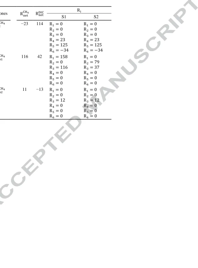
According to the reactions listed in Table 1, the in the sediments is given by:
where and are the rates of CH4 production due to acetate fermentation (r2) and hydrogenotrophy (r3), respectively; and is the rate of CO2 production due to CH4 oxidation (r4). For its part, the can be expressed as:
(3)
where and are the rates of CO2 production due to OM fermentation (r1) and oxidation (r5), respectively, and is the rate of siderite precipitation (r6).
3. RESULTS
3.1. Profiles of solute concentrations
The replicate depth distributions of CH4, δ13C-CH4, DIC, δ13C-DIC, , ΣS(−II) and Fe are shown in Fig. 1. The profiles do not display sharp discontinuities and the main vertical variations are defined by several data points, which suggests that differences among triplicate profiles should be mainly attributed to spatial variability within the 25 m2 sampling area and not to sampling and handling artefacts. Small-scale sediment patchiness is common in lakes (e.g., Downing and Rath, 1988; Brandl et al., 1993). Profiles of acetate are not shown because concentrations were < 2 µM over the entire sampling interval. Figure 1 also shows sharp CH4, DIC and Fe gradients above the SWI, indicating diffusion-dominated transport in stagnant overlying water, a feature not unusual in this lake basin (Clayer et al., 2016).
In the overlying water, concentrations are seven times lower than those
measured in the epilimnetic waters (Alfaro-De La Torre, 2001), and some of the ΣS(−II) concentrations are significantly higher than the detection limit (i.e., 0.02 µM, Fig. 1h), as often found when reduction occurs in anoxic waters. Below the SWI, ΣS(−II)
concentrations decrease and then remain relatively constant at a low concentration of 0.05 ± 0.02 µM, and concentrations remain lower than 3 μM (filled squares and
circles in Fig. 1g), except for one profile (filled triangles in Fig. 1g) where they increase with depth to a maximum at about 15 cm. The Fe profiles show sharp positive (top 3 cm)
and negative (between 2 and 5 cm) concentration gradients (Fig. 1i) which indicate dissolved Fe production and consumption, respectively. Below 5 cm depth, the concentrations progressively increase with depth.
The concentrations of CH4, which increase with depth from 0.2–0.5 mM in the overlying water to 1.2–1.4 mM at the base of the profiles (Fig. 1a–c), are well below saturation, i.e., 7.1 mM at 4°C and in situ pressure (Duan and Mao, 2006), suggesting that ebullition is a negligible transport process. The CH4 profiles follow two distinct patterns (Fig. 1a–c). Those represented by circles and squares consistently show a
concave-up curvature between 0 and 5–6 cm depth and a concave-down curvature below, whereas that symbolized by triangles displays a concave-down curvature over the entire sediment column. This disparity, also observed for the other solute concentrations and δ13
C data, where the profile represented by triangles is always different from the two others (Fig. 1), can be attributed to the heterogeneity at the study site (Brandl et al., 1993).
The CH4 concentration profile calculated with the code PROFILE accurately fits the average (n = 3) measured data (r2 > 0.998; Fig. 2a) and predicts a diffusive flux of CH4 ( pmol cm−2 s−1) to the bottom water. The profile shows a zone of net CH4 consumption ( ; fmol cm−3 s−1) above two zones of net
production, one located between 5 and 7.5 cm depth ( ; fmol cm−3 s−1) and the other below 7.5 cm depth ( ; fmol cm−3
s−1). The and can be combined into a single zone of net CH4 production by forcing the code PROFILE to rationalize the average CH4 profile with only two zones instead of three, but it
statistical F-testing at a level of significance ≤ 0.001 shows that the profile with three zones is significantly better than that with only two zones.
The concentrations of DIC, as those of CH4, increase steadily between the
overlying water and 23 cm depth (Fig. 1e). The code PROFILE generates a curve that fits accurately the average (n = 3) experimental DIC data (r2 > 0.998; Fig. 2b) and it predicts that the diffusive flux of DIC ( ) to the overlying water is pmol cm−2
s−1. It defines three zones of net DIC production or consumption numbered , and
from the sediment surface (Fig. 2b). Two zones of net DIC production ( and
where is equal to 138 fmol cm−3
s−1 and 42 fmol cm−3 s−1, respectively) occur above a zone of net DIC consumption ( , with
fmol cm−3
s−1). Note that the boundary between and does not match exactly that between and .
As a check of the robustness of the and depth distributions predicted
by PROFILE, the average CH4 and DIC profiles were also modeled using another inverse modeling code, i.e., Rate Estimation from Concentrations (REC, Lettmann et al., 2012). The REC code uses a statistical approach, the Tikhonov regularization technique, which differs from that used by PROFILE. Figure S1 in the Supplementary Material shows that the two codes predicted coherent rate profiles with the same number of zones, except for the two consecutive zones of DIC net production predicted by PROFILE, which are predicted by REC as a single zone of decreasing intensity. Moreover, the values of the net rates are of similar magnitude.
3.2. Profiles of δ13
C-CH4 and δ13C-DIC The δ13
C values increase with sediment depth from −74.2 ± 1.0‰ to
−70.7 ± 0.9‰ for CH4 (Fig. 1d) and from −13 ± 2.9‰ to +5.1 ± 0.9‰ for DIC (Fig. 1f). The values of δ13C-CH4, which are smaller than −70‰ over the whole sediment column, as well as the large difference between the δ13C of CO2 gas (δ13CO2) and δ13C-CH4 (68– 82‰), suggest that hydrogenotrophy is the main methanogenic pathway at our sampling site (Whiticar, 1999). These values differ from those reported for acetoclastic
methanogenesis (δ13C-CH4 from −68 to −50‰ and δ13CO2 − δ13C-CH4 from 39 to 58‰; Whiticar, 1999). The concomitant increase with depth of δ13C-CH4 and δ13C-DIC is consistent with a dominance of hydrogenotrophic methanogenesis. It should be noted that except for two data points (filled circles in Fig. 1d), the δ13C-CH4 signatures do not shift toward higher values in the or above the SWI (Figs. 1d and 3), a feature that is discussed in section 4.1.3. As shown in Fig. 3, the signature of all our samples falls within the CO2 reduction domain in a δ13CO2– δ13C-CH4 graph. Also, the δ2H of CH4 (−160 to −183‰ SMOW) is typical of CH4 produced by CO2 reduction (Whiticar, 1999).
4. DISCUSSION
4.1. Pathways of OM degradation
Plotting the experimental data on the δ13CO2 vs. δ13C-CH4 graph proposed by Whiticar (1999; see Fig. 3) allows performing a quick diagnosis of the main
methanogenic and methanotrophic pathways but is insufficient to quantify the relative contribution of each reaction involved in OM mineralization. To reach this goal, we select from Table 1 the reactions that are plausible in each zone, constrain their rates
using the and values reported in Table 2, and assign a rate value of 0 to the
reactions that are unlikely to occur. The sets of reaction rates thus established for r1 to r6 in each zone, when combined for the , and , provide scenarios to predict the δ13C-CH4 and δ13C-DIC profiles with a one-dimensional diagenetic reaction-transport equation. The comparison between the measured and simulated δ13C-CH4 and δ13C-DIC profiles allows to propose the most probable scenario and to quantify the contribution of each reaction to OM degradation. The diagenetic equation, conversely to the Rayleigh model, takes into account the influence of transport processes on the depth distribution of isotope ratios, and it is better suited from a theoretical point of view for constraining fractionation factors and diffusivity coefficients in sediments (Alperin et al., 1988).
4.1.1. Constraining the rates of OM mineralization reactions
In the (i.e., between the SWI and 5 cm depth), DIC is produced through both OM oxidation and methanotrophy as revealed by the value greater than that of
(Table 2). For now, we assume that fermentation and methanogenesis are negligible in the , i.e., , since these processes should only occur when EAs are absent (Bridgham et al., 2013). Shortage of EAs is unlikely because the porewater Fe profiles (Fig. 1i) reveal some Fe oxyhydroxide reduction in the , between 0 and 2 cm. In addition, below that depth interval, within the same zone, the Fe profiles display evidence of porewater Fe consumption, and SI values in that zone (SI ≥ 0.5) indicate that porewater is supersaturated with respect to siderite. Modeling the average Fe concentration profiles with the code PROFILE yields a net Fe consumption rate of −34 fmol cm−3 s−1 over the which is considered below as an estimate of the
rate of siderite precipitation, i.e., R6 = −34 fmol cm−3 s−1. With thie assumption stated above, the only reactions thus occurring in that zone are r4, r5 and r6. Consequently, Eq. 3 simplifies to fmol cm−3
s−1 and, from Eq. 4, we obtain that
fmol cm−3
s−1 (Table 2). The effect of adding methanogenesis to OM oxidation, methanotrophy and siderite precipitation in the is discussed below in section 4.1.3.
In the (i.e., between 5 and 7.5 cm depth), which is the zone with the most elevated net CH4 production rate, CH4 and DIC are simultaneously produced but the value of is more than twice that of (Fig. 2 and Table 2). Note that this
observation is consistent with our previous study at the same site showing similar values for the CH4 to DIC net rate ratios (
/
of 2 to 4) in the sediment methanogenic
zone (Clayer et al., 2016). We assume that reactions r4, r5 and r6 are not significant sources or sink of DIC, i.e., , leaving only reaction r1–r3 as plausible reactions in the . This assumption is based on the facts that nitrate and Mn
oxyhydroxides can be neglected as oxidants (see section 2.4) and that the porewater profiles of and Fe display only slight concentration variations within the 5–7.5 cm
depth interval (Fig. 1g and i). Modeling these profiles with Eq. 2 (data not shown) indicates that there is no net consumption (
) in the
and that the net
rate of dissolved Fe production in that zone (i.e., fmol cm−3
s−1), from which we may infer some Fe(III) reduction, is more than two orders of magnitude lower than that of the net rate of DIC production.
To avoid the complexity of testing a large number of hydrogenotrophy and acetate fermentation proportions for the CH4 production in the
, we consider two extreme cases (or end-members). For one of them, we postulate that methanogenesis proceeds exclusively through hydrogenotrophy, i.e., . In that case, r1 produces only CO2 and H2, but no acetate (i.e., x = ν in reaction r1), and we obtain, from Eq. 3, that
fmol cm−3
s−1 and, by adding Eqs. 3 and 4, that fmol cm−3 s−1. In the other extreme case, we constrain the maximum proportion of CH4 produced by acetate fermentation with the measured values of and considering
that all DIC is produced by this process, i.e., r1 produces only acetate and H2 (ν = 0 in reaction r1 and ). By adding Eqs. 3 and 4, we obtain
fmol cm−3 s−1 and, from Eq. 3, that fmol cm−3 s−1. In this extreme case (or end-member), the proportions of the total CH4 production through acetate fermentation and hydrogenotrophy are 68% (i.e., ) and 32% (i.e., ), respectively.
Lastly, in the (i.e., 7.5–22.5 cm depth), the net production rate of CH4 and the net consumption rate of DIC have a similar value (i.e., 11–13 fmol cm−3 s−1; Table 2) suggesting that hydrogenotrophy (r3) is the only reaction taking place in that zone. The presence of DIC in the is likely due to its diffusion from deeper porewater and perhaps from the (Fig. 2c), but not to its production through the reactions listed in Table 1. Since there is no evidence of siderite precipitation in that zone (i.e., ), and assuming that , it can be written from Eqs. 3 and 4 that
fmol cm−3
s−1. Note that the origin of the substrate H2 required for hydrogenotrophy is discussed below.
The values of the reaction rates R1–R6 evaluated as described above in the three zones defined by our modeling, are combined in order to provide two scenarios (S1 and S2) of reaction rates for the top 25 cm of Lake Tantaré sediments (see Table 2). While only one set of reaction rates is realistic for each of the and the , two sets are considered for the , corresponding to the maximum (S1) and minimum (S2) proportion of hydrogenotrophy. Below, the δ13C profiles of CH4 and DIC are simulated according to these scenarios.
4.1.2. Modeling the δ13
C-CH4 and δ13C-DIC profiles
To model the δ13C profiles of CH4 and DIC, we use Eq. 1 modified as follows:
where is the total CH4 or DIC concentration, which is an approximation of the
isotopically light concentrations of these solutes, given that ~99% of total carbon is made of 12C (Faure, 1998), and is the isotopically heavy CH4 or DIC concentration. Equation 5 allows calculating δ13C once and are known. A numerical representation of the depth distribution is given by Eq. 2, whereas that for is
obtained by an adapted version of Eq. 2 (Alperin et al., 1988), in which is
(5)
replaced by and by the net reaction rate of the isotopically heavy solute ( ):
where f, the molecular diffusivity ratio, is the diffusion coefficient of the total solute divided by that of the isotopically heavy solute (Table 3). In Eq. 6, is the sum of the reaction rates of the isotopically heavy solute in reactions r1–r6 (Table 1), i.e.,
. The rate can be expressed as follows (Rees, 1973):
(7)
where is the isotopic fractionation factor, and are the total
concentrations of a reactant and that of its isotopically heavy component, respectively, and is the solute reaction rate in reaction ri. Substituting Eq. 7 into Eq. 6, we obtain:
(8)
Introducing the definition of , i.e., the δ13
C of the reactant in reaction ri leading to the formation of the solute (CH4 or DIC), into Eq. 8 leads to:
(9). (6)
Equation 2 was solved numerically for via the bvp5c function of MATLAB® using , the measured , and or in the ,
and as inputs, and,
CH4 or DIC concentrations at the top and bottom of the profiles as boundary conditions. It should be noted that the value of in the used for the calculations was a weighted average of the two values provided by PROFILE in that zone (Fig. 2b, Table 2). The CH4 and DIC profiles simulated this way were very similar to those generated by the code PROFILE (Fig. 2a and b), thus validating our script.
With regard to Eq. 9, it was solved for via the bvp5c function of
MATLAB®, using , , , , and as inputs, and the values at the top and bottom of the profiles calculated with Eq. 5 as boundary conditions. The values of were those reported in Table 2 for scenarios S1 and S2. The values of
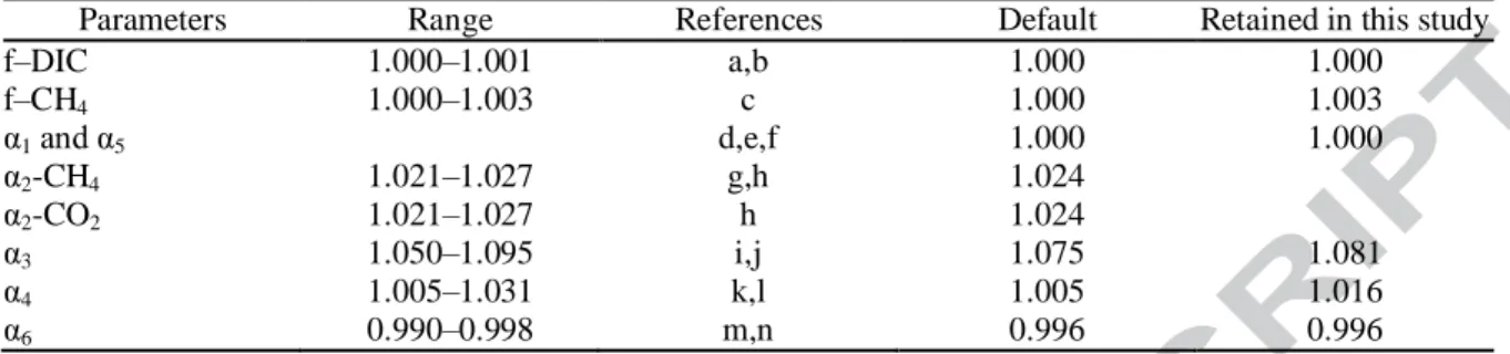
were −28‰ for OM (Joshani, 2015), −38‰ and −18‰ for the methyl and carboxyl groups of acetate (Conrad et al., 2014), respectively, and the measured values of δ13 C-CH4 and δ13C-DIC. We assumed no isotope fractionation during CO2 production through OM fermentation and oxidation (i.e., α1 = α5 = 1.000) as reported in many studies
(Lapham et al., 1999; Fey et al., 2004; Werth and Kuzyakov, 2010; Conrad et al., 2012). Considering the large ranges of values reported in the literature for α2, α3 and α4,
estimated values, hereafter referred to as default values, were selected for initial
simulations. Methane produced by acetate fermentation (r2) is typically depleted in 13C by 21–27‰ (i.e., α2-CH4 varies between 1.021 and 1.027) compared to its substrate, the methyl group of acetate (Krzycki et al., 1987; Gelwicks et al., 1994; Whiticar, 1999; Conrad, 2005), and CO2 production through acetoclastic methanogenesis appears to undergo similar 13C depletion (Blair and Carter, 1992; Gelwicks et al., 1994).
Consequently, the same intermediate fractionation factor was chosen as default values for α2-CH4 and α2-CO2 i.e., 1.024. Hydrogenotrophy is known to generate a larger
fractionation than acetate fermentation with α3 values ranging from 1.050 to 1.095 (Whiticar, 1999; Conrad, 2005). In agreement with Conrad et al. (2014), we used 1.075 as the default value for α3. As regard α4, a default value of 1.005 was selected as in Whiticar and Faber (1986) and in agreement with other studies showing that α4 may vary from 1.005 to 1.031 (Alperin et al., 1988; Whiticar, 1999). For siderite precipitation, we calculated a composite α6 value using the fractionation factors reported for calcite precipitation from aqueous CO2 (0.990) or (0.998) solutions and taking into account the relative proportions of porewater and CO2 concentrations (Bottinga, 1969; Emrich et al., 1970).
Isotopic fractionation due to diffusion depends on the mass and on the interaction among solute molecules and water (Jähne et al., 1987). The strong interactions between DIC and water lowers the theoretical kinetic fractionation effect resulting in an f-DIC value lower than 1.001 (O'Leary, 1984; Jähne et al., 1987). In contrast, a relatively higher value is expected for f-CH4 because of the relatively large mass difference between 13CH4 and 12CH4 compared with that between 13CO2 and 12CO2, and the weaker interactions between CH4 and water due to the hydrophobic character of CH4. The value of f–CH4 was estimated to be less than 1.003 at the water-air interface (Happell et al., 1995), which can be considered as a maximum value in sediments. We thus chose 1.000 as default value for f-CH4 and f-DIC. After performing the initial simulation, the values of f-CH4, as well as those of α2, α3 and α4, were then varied within the ranges reported in the literature (Table 3) to perform additional simulations.
The depth distributions of and were combined in Eq. 5 to model the
δ13
C profiles of CH4 and DIC, which were visually and statistically compared to the measured profiles to determine what scenario and parameter values best reflect the measurements. The norm of residuals ( ) was used to compare the goodness of fits:
(10)
where and are the measured and simulated δ13
C values, respectively. The norm of residuals ( ) varies between 0 and infinity with smaller numbers indicating better fits.
4.1.3. Selecting the best scenario
Figure 4 shows that the δ13C-CH4 and δ13C-DIC profiles modeled with default parameters result in a better fit of the measured profiles for S1 than for S2. Indeed, the Nres values of δ13C-CH4 (1.09) and δ13C-DIC (1.65) for S1 are lower than those for S2 (≥ 3.70). The search for the best scenario can be taken a step further by investigating the influence of the fractionation factors α2, α3, and α4, and of the molecular diffusivity factor f-CH4 on Nres.
The fit between the measured and modeled δ13C-CH4 profiles for scenario S2 can be improved by varying α3 within the range of values given in Table 3, while maintaining the default values for the other parameters; the best fit is obtained with α3 = 1.087
(Nres = 0.84). However, the Nres for δ13C-DIC remained above 4.90 regardless of the α3 value. Varying the other parameters between their maximum and minimum values
reported in Table 3 together with that of α3 did not significantly improve the δ13C-DIC fit (Nres> 4.00). We thus conclude that scenario S2 is unrealistic and it is not discussed further.
Figure 5a shows that varying α3, the most influential fractionation factor for scenario S1, and maintaining the default values for the other parameters, can significantly improve the fit between measured and simulated profiles. However, the minimum value of Nres occurs at different α3 values for the δ13C-CH4 (α3 = 1.0764) and the δ13C-DIC (α3 = 1.0830) profiles, likely due errors associated with the analyses and estimation of the rates. Given that α3 ought to have the same value for both δ13C-CH4 and δ13C-DIC, the best fit is considered to occur at the minimum of total Nres (the sum of Nres for the δ13 C-CH4 and the δ13C-DIC profiles), i.e., at α3 = 1.0770 in Fig. 5a where total Nres is 2.23. Increasing the value of f-CH4 from 1.000 to 1.003 and that of α4 from 1.005 to 1.016 further lowers the minimum total Nres value to 1.89 at α3 = 1.081. This latter value of total Nres correspond to the best fit of the modeled profiles that we can obtain for S1.
The better fit for S1 compared to S2 agrees with the predominance of
hydrogenotrophy in CH4 production in Lake Tantaré sediments, but to estimate more precisely the contribution of acetate fermentation to methanogenesis, additional
simulations were performed by varying the proportion of acetoclastic methanogenesis in the from 0 (as in S1) to 25%. For each proportion of acetoclastic methanogenesis tested, the values of α2, α3, α4 and f-CH4 were optimized, as done for S1. Increasing the proportion of acetate fermentation slightly lowers the Nres values of the δ13C-CH4 fit but
increases considerably that of the δ13C-DIC fit (Fig. 5b), which indicates that the contribution of acetate fermentation is negligible in the .
The value of α3 yielding the best fit (1.081) is well within the range reported in the literature (Table 3). This value is slightly higher than that (1.075) estimated from incubation experiments usually performed at temperatures above 20°C (Conrad et al., 2014). The lower temperature (4°C) at the study site could explain our slightly greater α3 value since this fractionation factor is reported to decrease with temperature (Richet et al., 1977; Whiticar et al., 1986). Lastly, our optimal value for α4 (1.016) is within the range reported for aerobic CH4 oxidation (Barker and Fritz, 1981). However, it remains poorly constrained considering that only a minor fraction of CH4 is consumed through oxidation in the .
Methanogenesis in the needs to be invoked to explain the upward decrease in δ13C-CH4 in that zone, which is at odds with the assumption that made in developing S1 and S2 (section 4.1.1.). Strong 13C-CH4 depletion is often
observed near the base of the sulfate methane transition zone, where CH4 is consumed via reduction in marine sediments (Borowski et al., 1997; Martens et al., 1999;
Pohlman et al., 2008; Treude et al., 2014). This feature, which is counterintuitive since the CH4 left behind during methanotrophy should be 13C-enriched, has been attributed to the production of CH4 by hydrogenotrophy from the 13C-depleted DIC resulting from anaerobic CH4 oxidation (Borowski et al., 1997; Pohlman et al., 2008). In our case, we suggest that the 13C-CH4 depletion in the results mainly from reduction of 13 C-depleted DIC originating from the oxidation of OM (δ13C = −28‰; Joshani 2015), the
main source of DIC in that zone (Table 2). This contention is supported by: i) the positive correlation between δ13C-CH4 and δ13C-DIC in the
(Fig. 2 c and d), ii) the δ13C values for CH4 (−74 to −72‰) and CO2 gas (−2 to 6‰) in that zone which plot in the hydrogenotrophy domain in Fig. 3, and iii) the difference between δ13CO2 and δ13C-CH4 (68–73‰) which is typical of hydrogenotrophy (Whiticar, 1999). Note that this
difference is smaller in the than in the and (74–83‰) in which hydrogenotrophy is the main reaction, suggesting that methanotrophy is occurring in addition to hydrogenotrophy in the . Sediments are naturally heterogeneous and microenvironments of redox potential lower than that of the bulk sediment, where OM fermentation and hydrogenotrophy could occur, are likely present in the . A small contribution of hydrogenotrophy would probably be sufficient to counterbalance the 13 C-CH4 enrichment expected from methanotrophy and produce the observed net 13C-CH4 depletion since isotopic fractionation is much greater for hydrogenotrophy than for methanotrophy. Adding hydrogenotrophy in the at rates of up to 30 fmol cm−3 s−1, i.e., up to 55% of the rate of methanotrophy, slightly worsens the fits of the measured δ13
C-CH4 and δ13C-DIC (Nres ≤ 1.94) compared to those obtained for S1 (Nres =1.89). Also, only minor changes in the values of the fractionation factors were required to optimize the fits when adding hydrogenotrophy. The optimized α values remain within the ranges given in Table 3. In addition, the total Nres increased when acetoclastic methanogenesis was added, as it was the case when hydrogenotrophy was neglected in the .
4.2. Sources of H2 in the zones of CH4 production
The dominant substrates in fermentation, often inferred to be polysaccharides (Conrad, 1999), are commonly represented in geochemical models by the simple molecule CH2O (Van Cappellen and Wang, 1996; Canavan et al., 2006; Conrad et al., 2009; Conrad et al., 2010; Galand et al., 2010; Corbett et al., 2013; Aller, 2014; Arning et al., 2016), whose complete fermentation, coupled to methanogenesis, yield equimolar amounts of CH4 and CO2. The fermentation of CH2O, coupled to hydrogenotrophy, cannot alone explain the facts that is about three times greater than in the
, and that DIC is consumed at about the same rate as CH4 is produced in the (Table 2). Additional H2 production is thus required at rates of 148 fmol cm−3 s−1 and of 48 fmol cm−3 s−1, i.e., four times the missing CH4 production rate of ,
in the and , respectively. The importance of a cryptic Fe-S cycle (Mills et al., 2016) and of the fermentation of organic substrates which are more reduced than CH2O, as possible pathways of additional H2 production, are discussed below.
4.2.1. The importance of a cryptic Fe-S cycle
The reduction of Fe oxyhydroxides coupled to the oxidation of reduced sulfur, also referred to as a cryptic Fe-S cycle (Bottrell et al., 2000; Holmkvist et al., 2011a; Holmkvist et al., 2011b; Mills et al., 2016), could produce some H2:
(11)
(12)
where R7 and R8 are the rates of solid Fe(III) reduction via reactions 11 and 12, respectively.
Reactions 11 and 12 may occur in the sediment below the as revealed by the progressive downward increases in dissolved Fe (Fig. 1i) and of (Fig. 1g) with depth, which suggests that solid-phase Fe(III) reduction continues to be effective below the , and that is coincidently produced as in reaction 11. However, as estimated
in other studies (Liu et al., 2015; Clayer et al., 2016), the rate of solid Fe(III)
consumption at our study site is too small, i.e., < 1 fmol cm−3 s−1, to provide enough H2 to sustain the required additional hydrogenotrophy in both the and . Indeed, to match the needed rate of H2 production, R7 should be 148 fmol cm−3 s−1 in the
, and 48 fmol cm−3 s−1 in the , whereas R8 should be twice these values. It may therefore be concluded that, if a cryptic Fe-S cycle is active in Lake Tantaré sediments, it cannot sustain the observed CH4 production rate.
4.2.2. The importance of reduced OM
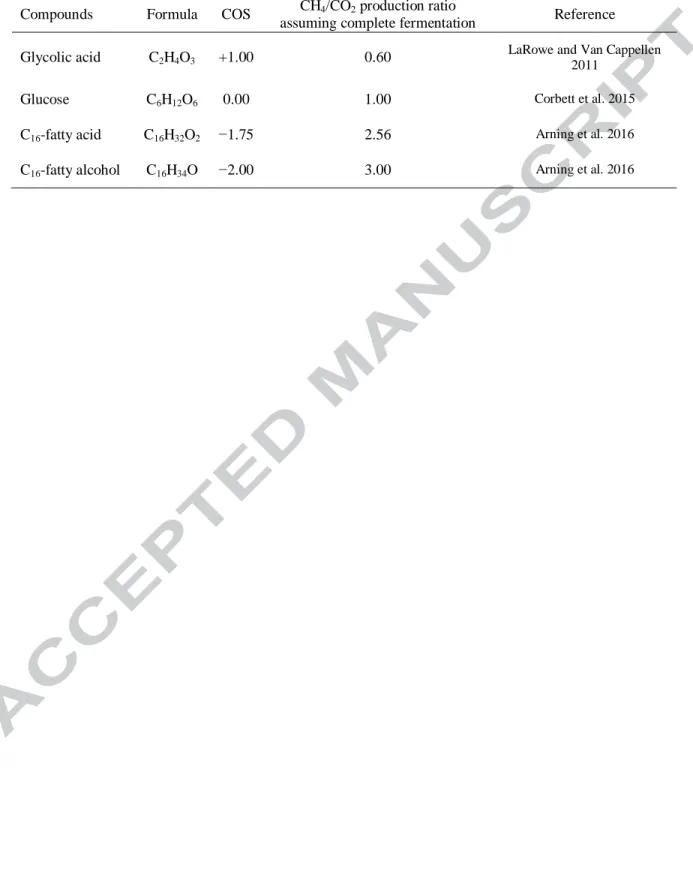
Metabolizable organic substrates other than carbohydrates, such as lipids, whose average carbon oxidation states (COS) is lower than 0, are likely abundant enough in sediments (Hedges and Oades, 1997; Burdige, 2006) to contribute significantly to the amount of CH4 and DIC produced during fermentation. The closer the COS of the fermenting molecules is to that of CH4 (COS = −4), the larger is the CH4 : CO2
production ratio (Arning et al., 2016; Table 4). For example, the complete fermentation of the C16-fatty acid (COS = −1.75) or any fatty alcohol (COS = −2.00) coupled to methanogenesis would yield 2.6–3.0 times more CH4 than CO2 (Table 4).
The stoichiometry and the COS of the fermenting OM ( ) can be
coupled. Note that this exercise does not apply to the since the substrate DIC required for hydrogenotrophy is not produced in that zone but diffuses from deeper sediments. Considering that methanogenesis is essentially hydrogenotrophic (i.e., x = ν), the reaction of fermentation (r1) becomes:
(13) If there is no other source of CO2, H2 and CH4 than the complete fermentation of CxHyOz and hydrogenotrophy, and if we assume that (Table 2), the rate of CO2 production in Eq. 13, i.e., R1, should be:
(14) and the rate of H2 production in Eq. 13 required to sustain the rate of CH4 production by reaction r3 can be written:
(15)
Introducing into Eq. 15, the values of (116 fmol cm−3 s−1; Table 2) and that of R1 (158 fmol cm−3 s−1; Eq. 14), we obtain:
(16)
The COS of an organic molecule is given by:
(17)
where OSi is the oxidation state of the element i and ni/nc is its molar ratio to carbon.
Assuming that the COS of the fermenting molecule in the is defined only by H and O atoms, it can be written:
(18) This COS value is closer to those of fatty acids (COS of −1.50 for C8-fatty acids to about −1.87 for C32-fatty acids) and of fatty alcohols (COS = −2.00) than to that of the
commonly assumed model organic molecule CH2O (COS = 0). Fatty acids are
widespread lipid compounds in lake sediments (Cranwell, 1981; Matsumoto, 1989), and the short-chain (up to 20 C) acids are known to be more labile than their long-chain counterparts (Farrington et al., 1977; Matsuda and Koyama, 1977; Matsuda, 1978) with molecules containing 16 C atoms being the most abundant (Cranwell, 1981; Matsumoto, 1989).
From Eq. 16, the general formula for the fermenting OM can be written:
. Given that a carbon chain of x atoms can be bound to a maximum of (2x
+ 2) H or O atoms, we can write:
(19)
Combining Eqs. 16 and 19 leads to:
(20)
If we assume that the number of C atoms in the fermenting OM is 16, its formula becomes with , and the sum of the reactions of fermentation
(Eq. 13) and hydrogenotrophy (r3) could thus be written as follows:
(21)
r3
(22)
Equations 18 and 22 were developed with the assumption that there was no other source of CH4, H2 and CO2 than fermentation and hydrogenotrophy in the
.
Increasing the rate of methanotrophy, and that of hydrogenotrophy by the same value in order to remain consistent with the measured value of and with Eq. 3, would increase the rate of H2 production required in Eq. 21 to sustain the CH4 production rate. More H atoms would thus be required in the chemical formula of the fermenting OM, which would decrease its COS. Considering that EAs are depleted in the as discussed in section 4.1.1., and that adding some methanotrophy in that zone would not improve the fit between simulated and measured δ13
C profiles (data not shown), there is no reason to believe that methanotrophy is a significant source of DIC in the . Lastly, in deriving the COS, we assumed that the fermenting molecules contain only C, H and O. Including other elements (e.g., N and S) would have only a minor effect on the COS value because these elements are not abundant.
Although, the accuracy of the COS value (−1.9) estimated with Eq. 18 is difficult to evaluate, such low COS values can only be explained by the fermentation of fatty acids and alcohols, terpenes or complex reduced organics such as type I kerogen (Kroll et al., 2011; LaRowe and Van Cappellen, 2011). Complex organic molecules are generally considered non-degradable, especially under anoxic conditions (Burdige, 2007). Although it is generally accepted that lipids are less degradable than proteins or
carbohydrates (Baldock et al., 2004; LaRowe and Van Cappellen, 2011), several studies showed that fatty acids and sterols are degraded in natural sediments under anoxic conditions (Farrington et al., 1977; Kawamura et al., 1980; Cranwell, 1981; Canuel and Martens, 1996; Harvey and Macko, 1997). We thus submit that once organic particles
reach the sediment floor at our study site, the most easily degradable organic compounds (i.e., proteins and carbohydrates) are rapidly degraded within the , leaving mainly lipids and fatty alcohols as degradable substrates in the for fermentation and methanogenesis.
Considering that the Corg represents ~20% of the dry sediment mass of the
oligotrophic Lake Tantaré, i.e., that about 40% of the sediment is organic, fermentation of compounds, such as lipids, which is considered negligible in marine settings, can be a significant source of mineralized carbon in these lake sediments.
5. CONCLUSIONS
Modeling the concentrations and δ13C profiles of CH4 and DIC with reaction-transport equations reveals that OM fermenting in the sediments of a seasonally anoxic lacustrine basin is more reduced than CH2O and yields significantly more CH4 than DIC. We propose that the organic substrates undergoing fermentation can be represented by the general formula , where z can take any value between 0 and
(0.13x+2)/3. While this chemical formula is more representative of the OM fermenting in the sediments of our study site than CH2O, its general applicability to boreal lake
sediments remains to be demonstrated. If suitable for sediments deposited under other redox conditions, the current formulation of the fermenting OM in geochemical models, i.e., CH2O, should be revised for better predictions of CH4 cycling in boreal lakes.
The accurate fitting between the measured and modeled δ13
C-CH4 and δ13C-DIC profiles also allows quantifying in situ OM mineralization reaction rates including those of each methanogenesis pathway, and constraining the carbon isotope fractionation
factors of several OM mineralization reactions occurring under natural conditions. We conclude that nearly all of the CH4 production in the sediments of our seasonally anoxic lacustrine basin is derived from hydrogenotrophy. A proposed explanation to rationalize the shifts in CH4 production from acetoclastic to hydrogenotrophic methanogenesis with sediment/soil depth (Hornibrook et al., 1997; Conrad et al., 2009), as well as with variations in primary production (Wand et al., 2006; Galand et al., 2010), is that hydrogenotrophy becomes predominant when labile OM is depleted (Whiticar et al., 1986; Chasar et al., 2000; Hornibrook et al., 2000). Our observation that the
predominance of the hydrogenotrophic pathway is associated with a negative COS value (−1.87) of the fermenting OM, i.e., implying that labile organic substrates such as carbohydrates and proteins are depleted, is a strong support for this interpretation. In the seasonally anoxic basin of our oligotrophic lake, the labile fraction of OM is rapidly degraded near the SWI, leaving only reduced organic compounds, i.e., lipids and fatty alcohols, to sustain hydrogenotrophy deeper in the sediments. Given the low rates of primary production in most boreal lakes and the terrigenous origin of their OM, it would not be surprising, as suggested by Hornibrook et al. (2000), that hydrogenotrophy dominates CH4 production in the sediments of these lakes.
Acknowledgements
We thank L. Rancourt, P. Girard, J.-F. Dutil, S. Duval, A. Royer-Lavallée, A. Laberge and A. Barber for laboratory and field work assistance, and three anonymous reviewers whose comments contributed to significantly improve this manuscript. We are thankful to J.-F. Hélie, from the Laboratoire de géochimie des isotopes stables légers (UQÀM), who graciously calibrated our δ13C internal standard. This work was supported
by grants to C.G., A.T. and Y.G. from the Natural Sciences and Engineering Research Council of Canada and the Fonds de Recherche Québécois – Nature et Technologies. Permission from the Québec Ministère du Développement durable, de l’Environnement et de la Lutte contre les changements climatiques to work in the Tantaré Ecological Reserve is gratefully acknowledged.
References
Alfaro-De La Torre M. C. (2001) Géochimie du cadmium dans un lac oligotrophe acide. Ph.D. thesis, INRS-EAU, Université du Québec.
Aller R. C. (2014) Sedimentary diagenesis, depositional environments, and benthic fluxes. In Treatise on Geochemistry (eds. Holland H. and Turekian K.) 2nd ed., Elsevier, Oxford. pp. 293-334.
Alperin M. J., Reeburgh W. S. and Whiticar M. J. (1988) Carbon and hydrogen isotope fraction resulting from anaerobic methane oxidation. Global Biogeochem. Cycles
2, 279-288.
Alperin M. J., Albert D. B. and Martens C. S. (1994) Seasonal variations in production and consumption rates of dissolved organic carbon in an organic-rich coastal sediment. Geochim. Cosmochim. Acta 58, 4909-4930.
Arndt S., Jørgensen B. B., LaRowe D. E., Middelburg J. J., Pancost R. D. and Regnier P. (2013) Quantifying the degradation of organic matter in marine sediments: A review and synthesis. Earth-Sci. Rev. 123, 53-86.
Arning E. T., van Berk W. and Schulz H.-M. (2016) Fate and behaviour of marine organic matter during burial of anoxic sediments: Testing CH2O as generalized input parameter in reaction transport models. Mar. Chem. 178, 8-21.
Baldock J. A., Masiello C. A., Gélinas Y. and Hedges J. I. (2004) Cycling and
composition of organic matter in terrestrial and marine ecosystems. Mar. Chem.
92, 39-64.
Barker J. F. and Fritz P. (1981) Carbon isotope fractionation during microbial methane oxidation. Nature 293, 289-291.
Bastviken D., Cole J., Pace M. and Tranvik L. (2004) Methane emissions from lakes: Dependence of lake characteristics, two regional assessments, and a global estimate. Global Biogeochem. Cycles 18.
Berelson W. M., Prokopenko M., Sansone F. J., Graham A. W., McManus J. and Bernhard J. M. (2005) Anaerobic diagenesis of silica and carbon in continental margin sediments: Discrete zones of TCO2 production. Geochim. Cosmochim.
Acta 69, 4611-4629.
Berg P., Risgaard-Petersen N. and Rysgaard S. (1998) Interpretation of measured
concentration profiles in sediment pore water. Limnol. Oceanogr. 43, 1500-1510. Berner R. A. (1980) Early Diagenesis: A Theoretical Approach. Princeton University
Press, Princeton, New Jersey.
Blair N. E. and Carter J. W. D. (1992) The carbon isotope biogeochemistry of acetate from a methanogenic marine sediment. Geochim. Cosmochim. Acta 56, 1247-1258.
Borowski W. S., Paull C. K. and Ussler W. (1997) Carbon cycling within the upper methanogenic zone of continental rise sediments; An example from the methane-rich sediments overlying the Blake Ridge gas hydrate deposits. Mar. Chem. 57, 299-311.
Bottinga Y. (1968) Calculation of fractionation factors for carbon and oxygen isotopic exchange in the system calcite-carbon dioxide-water. J. Phys. Chem. 72, 800-808.
Bottrell S.H., Parkes R. J., Cragg B. A. and Raiswell R. (2000) Isotopic evidence for anoxic pyrite oxidation and stimulation of bacterial sulphate reduction in marine sediments. J. Geol. Soc. (London, U. K.) 157, 711-714.
Boudreau B. P. (1997) Diagenetic Models and their Implementation: Modelling
Transport and Reactions in Aquatic Sediments. 1st ed. Springer, Berlin.
Brandl H., Hanselmann K.W., Bachofen R. and Piccard J. (1993) Small-scale patchiness in the chemistry and microbiology of sediments in Lake Geneva, Switzerland. J.
Gen. Microb. 139, 2271-2275.
Bridgham S. D., Cadillo-Quiroz H., Keller J. K. and Zhuang Q. (2013) Methane
emissions from wetlands: Biogeochemical, microbial, and modeling perspectives from local to global scales. Glob. Chang. Biol. 19, 1325-1346.
Burdige D. J. (2006) Geochemistry of Marine Sediments. Princeton University Press, Princeton and Oxford.
Burdige D. J. (2007) Preservation of organic matter in marine sediments: Controls, mechanisms, and an imbalance in sediment organic carbon budgets? Chem. Rev.
107, 467-485.
Burdige D. J. and Komada T. (2011) Anaerobic oxidation of methane and the stoichiometry of remineralization processes in continental margin sediments.
Limnol. Oceanogr. 56, 1781-1796.
Canavan R. W., Slomp C. P., Jourabchi P., Van Cappellen P., Laverman A.M. and van den Berg G.A. (2006) Organic matter mineralization in sediment of a coastal freshwater lake and response to salinization. Geochim. Cosmochim. Acta 70, 2836-2855.
Canuel E. A. and Martens C. S. (1996) Reactivity of recently deposited organic matter: Degradation of lipid compounds near the sediment-water interface. Geochim.
Cosmochim. Acta 60, 1793-1806.
Carignan R., Rapin F. and Tessier A. (1985) Sediment porewater sampling for metal analysis–a comparison of techniques. Geochim. Cosmochim. Acta 49, 2493-2497. Chanton J. P. (2005) The effect of gas transport on the isotope signature of methane in
wetlands. Org. Geochem. 36, 753-768.
Chanton J. P., Fields D. and Hines M. E. (2006) Controls on the hydrogen isotopic composition of biogenic methane from high-latitude terrestrial wetlands. J.
Geophys. Res.: Biogeosci. 111.
Chappaz A., Gobeil C. and Tessier A. (2008) Geochemical and anthropogenic enrichments of Mo in sediments from perennially oxic and seasonally anoxic lakes in Eastern Canada. Geochim. Cosmochim. Acta 72, 170-184.
Chasar L. S., Chanton J. P., Glaser P. H. and Siegel D. I. (2000) Methane concentration and stable isotope distribution as evidence of rhizospheric processes: Comparison of a fen and bog in the Glacial Lake Agassiz Peatland complex. Annals of Botany
86, 655-663.
Clayer F., Gobeil C. and Tessier A. (2016) Rates and pathways of sedimentary organic matter mineralization in two basins of a boreal lake: Emphasis on methanogenesis and methanotrophy. Limnol. Oceanogr.
Conrad R. (1999) Contribution of hydrogen to methane production and control of
hydrogen concentrations in methanogenic soils and sediments. FEMS Microbiol.
Conrad R. (2005) Quantification of methanogenic pathways using stable carbon isotopic signatures: a review and a proposal. Org. Geochem. 36, 739-752.
Conrad R., Claus P. and Casper P. (2009) Characterization of stable isotope fractionation during methane production in the sediment of a eutrophic lake, Lake Dagow, Germany. Limnol. Oceanogr. 54, 457-471.
Conrad R., Claus P. and Casper P. (2010) Stable isotope fractionation during the
methanogenic degradation of organic matter in the sediment of an acidic bog lake, Lake Grosse Fuchskuhle. Limnol. Oceanogr. 55, 1932-1942.
Conrad R., Klose M., Yuan Q., Lu Y. and Chidthaisong A. (2012) Stable carbon isotope fractionation, carbon flux partitioning and priming effects in anoxic soils during methanogenic degradation of straw and soil organic matter. Soil Biol. Biochem.
49, 193-199.
Conrad R., Claus P., Chidthaisong A., Lu Y., Fernandez Scavino A., Liu Y., Angel R., Galand P. E., Casper P., Guerin F. and Enrich-Prast A. (2014) Stable carbon isotope biogeochemistry of propionate and acetate in methanogenic soils and lake sediments. Org. Geochem. 73, 1-7.
Corbett J. E., Tfaily M. M., Burdige D. J., Glaser P. H. and Chanton J. P. (2015) The relative importance of methanogenesis in the decomposition of organic matter in northern peatlands. J. Geophys. Res.: Biogeosci. 120, 280-293.
Corbett J. E., Tfaily M. M., Burdige D. J., Cooper W. T., Glaser P. H. and Chanton J. P. (2013) Partitioning pathways of CO2 production in peatlands with stable carbon isotopes. Biogeochemistry 114, 327-340.
Couture R. M., Gobeil C. and Tessier A. (2008) Chronology of atmospheric deposition of arsenic inferred from reconstructed sedimentary records. Environ. Sci. Technol.
42, 6508-6513.
Couture R.-M., Fischer R., Van Cappellen R. and Gobeil C. (2016) Non-steady state diagenesis of organic and inorganic sulfur in lake sediments. Geochim.
Cosmochim. Acta 194, 15-33.
Cranwell P.A. (1981) Diagenesis of free and bound lipids in terrestrial detritus deposited in a lacustrine sediment. Org. Geochem. 3, 79-89.
Downing J. A. and Rath L. C. (1988) Spatial patchiness in the lacustrine sedimentary environment. Limnol. Oceanogr. 33, 447-458.
Duan Z. and Mao S. (2006) A thermodynamic model for calculating methane solubility, density and gas phase composition of methane-bearing aqueous fluids from 273 to 523K and from 1 to 2000bar. Geochim. Cosmochim. Acta 70, 3369-3386.
Emrich K., Ehhalt D. H. and Vogel J. C. (1970) Carbon isotope fractionation during the precipitation of calcium carbonate. Earth Planet. Sci. Lett. 8, 363-371.
Farrington J. W., Henrichs S. M. and Anderson R. (1977) Fatty wids and Pb210
geochronology of a sediment core from Buzzards Bay, Massachusetts. Geochim.
Cosmochim. Acta 41, 289-296.
Faure G. (1998) Principles and Applications of Geochemistry. 2nd ed., Prentice Hall. Fey A., Claus P. and Conrad R. (2004) Temporal change of 13C-isotope signatures and
methanogenic pathways in rice field soil incubated anoxically at different temperatures. Geochim. Cosmochim. Acta 68, 293-306.
Galand P. E., Yrjälä K. and Conrad R. (2010) Stable carbon isotope fractionation during methanogenesis in three boreal peatland ecosystems. Biogeosciences 7, 3893-3900.
Gelwicks J. T., Risatti J. B. and Hayes J. M. (1994) Carbon Isotope Effects Associated with Aceticlastic Methanogenesis. Appl. Environ. Microbiol. 60, 467-472.
Happell J. D., Chanton J. P. and Showers W. J. (1995) Methane transfer across the water-air interface in stagnant wooded swamps of Florida: Evaluation of mass-transfer coefficients and isotopic fractionation. Limnol. Oceanogr. 40, 290-298.
Hare L., Carignan R. and Huerta-Diaz M. A. (1994) A field study of metal toxicity and accumulation by benthic invertebrates; Implications for the acid-volatile sulfide (AVS) model. Limnol. Oceanogr. 39, 1653-1668.
Harvey H. R. and Macko S. A. (1997) Kinetics of phytoplankton decay during simulated sedimentation: Changes in lipids under oxic and anoxic conditions. Org.
Geochem. 27, 129-140.
Hayduk W. and Laudie H. (1974) Prediction of diffusion coefficients for nonelectrolytes in dilute aqueous solutions. AlChE J. 20, 611-615.
Hedges J. I. and Oades J. M. (1997) Comparative organic geochemistries of soils and marine sediments. Org. Geochem. 27, 319-361.
Hedges J. I., Baldock J. A., Gelinas Y., Lee C., Peterson M. L. and Wakeham S. G. (2002) The biochemical and elemental compositions of marine plankton: A NMR perspective. Mar. Chem. 78, 47-63.
Hélie J.-F. (2004) Géochimie et flux de carbone organique et inorganique dans les
milieux aquatiques de l’est du Canada : exemples du Saint-Laurent et du réservoir Robert-Bourassa -approche isotopique -. Ph.D. thesis, Université du Québec à Montréal.
Hesslein R. H. (1976) Insitu sampler for close interval pore water studies. Limnol.
Oceanogr. 21, 912-914.
Holmkvist L., Ferdelman T. G. and Jørgensen B. B. (2011a) A cryptic sulfur cycle driven by iron in the methane zone of marine sediment (Aarhus Bay, Denmark).
Geochim. Cosmochim. Acta 75, 3581-3599.
Holmkvist L., Kamyshny A., Vogt C., Vamvakopoulos K., Ferdelman T. G. and
Jørgensen B. B. (2011b) Sulfate reduction below the sulfate–methane transition in Black Sea sediments. Deep-Sea Res. Pt I 58, 493-504.
Hornibrook E. R. C., Longstaffe F. J. and Fyfe W. S. (1997) Spatial distribution of microbial methane production pathways in temperate zone wetland soils: Stable carbon and hydrogen isotope evidence. Geochim. Cosmochim. Acta 61, 745-753. Hornibrook E. R. C., Longstaffe F. J. and Fyfe W. S. (2000) Evolution of stable carbon
isotope compositions for methane and carbon dioxide in freshwater wetlands and other anaerobic environments. Geochim. Cosmochim. Acta 64, 1013-1027. IPCC (2013) Climate change 2013 : the physical science basis. In Contribution of
Working Group I to the Fifth Assessment Report of the Intergovernmental Panel on Climate Change. (eds. Stocker T. F., Qin D., Plattner G.-K., Tignor M., Allen
S. K., Boschung J., Nauels A., Xia Y., Bex V. and Midgley P. M.). Cambridge University Press, Cambridge, UK, and New York, USA.
Jähne B., Heinz G. and Dietrich W. (1987) Measurement of the diffusion coefficients of sparingly soluble gases in water. J. Geophys. Res. 92, 10767-10776.