Towards sodium combustion modelling with liquid water

HAL Id: hal-02082710

https://hal.archives-ouvertes.fr/hal-02082710

Submitted on 28 Mar 2019

HAL is a multi-disciplinary open access archive for the deposit and dissemination of sci-entific research documents, whether they are pub-lished or not. The documents may come from teaching and research institutions in France or abroad, or from public or private research centers.

L’archive ouverte pluridisciplinaire HAL, est destinée au dépôt et à la diffusion de documents scientifiques de niveau recherche, publiés ou non, émanant des établissements d’enseignement et de recherche français ou étrangers, des laboratoires publics ou privés.

Towards sodium combustion modelling with liquid water

Damien Furfaro, Richard Saurel, Lucas David, François Beauchamp

To cite this version:

Damien Furfaro, Richard Saurel, Lucas David, François Beauchamp. Towards sodium combustion modelling with liquid water. Journal of Computational Physics, Elsevier, In press. �hal-02082710�

1

Towards sodium combustion modelling with liquid water

Damien Furfaro (1)_{, Richard Saurel} (1,2)_{, Lucas David} (2,3) _{and François Beauchamp} (3) (1) _{RS2N SAS, Saint Zacharie, France}

(2) _{Aix Marseille Univ, CNRS, Centrale Marseille, LMA, Marseille, France} (3) _{CEA Cadarache, LTRS, Saint-Paul-lez-Durance, France}

Abstract

Solid and liquid sodium combustion with liquid water occurs through a thin gas layer where exothermic reactions happen with sodium and water vapors. It thus involves multiple interfaces separating liquid and gas in the presence of surface tension, phase transition and surface reactions. The gas phase reaction involves compressible effects resulting in possible shock wave appearance in both gas and liquid phases. To understand and predict the complexity of sodium combustion with water a diffuse interface flow model is built. This formulation enables flow resolution in multidimension in the presence of complex motion, such as for example Leidenfrost-type thermo-chemical flow. More precisely sodium drop autonomous motion on the liquid surface is computed. Various modelling and numerical issues are present and addressed in the present contribution. In the author’s knowledge, the first computed results of such type of combustion phenomenon in multidimensions are presented in this paper thanks to the diffuse interface approach. Explosion phenomenon is addressed as well and is reproduced at least qualitatively thanks to extra ingredients such as turbulent mixing of sodium and water vapors in the gas film and delayed ignition. Shock wave emission from the thermo-chemical Leidenfrost-type flow is observed as reported in related experiments.

emails :

damien.furfaro@rs2n.eu richard.saurel@univ-amu.fr lucas.david@cea.fr

2

1. Introduction

Fast-neutron reactors (FNR) as well as other engineering systems use sodium (N_a) as coolant fluid. Sodium presents excellent physical properties regarding heat transfer efficiency as well as its ability to maintain kinetic energy of fast neutrons. However, it has major drawbacks regarding safety issues as it reacts exothermically with both air and water. In the limit, explosion may occur resulting in shock wave propagation in the liquid and surrounding media.

When a liquid or solid sodium drop is set on a liquid water surface surprising phenomenon occurs. A reaction appears rapidly resulting in autonomous drop motion on the liquid surface. It seems that the drop is separated from liquid water by a small gas layer where combustion occurs both in the gas phase and at sodium surface. The phenomenon is reminiscent of the Leidenfrost effect except that the heat needed to vaporize sodium and water comes from the combustion of themselves or their vapors. This combustion induces liquid water evaporation and heating of the sodium drop. After some delay, typically a few seconds, explosion occurs. These complex events are qualitatively reported on many videos available on the web, such as [www.youtube.com/watch?v=ODf_sPexS2Q] for example. They clearly illustrate complexity of the physics and chemistry in presence.

Quantitative analytic experiments have been carried out at CEA Cadarache, France, in the facilities SOCRATE, DINAMO, VIPERE and LAVINO (Carnevali 2012, Carnevali et al. 2013, Daudin 2015, Daudin et al. 2018, David et al. 2019).

These experiments confirm an important fact: liquid sodium and liquid water are always separated by a gas layer or bubbly zone, resulting in significant lowering of the energy release efficiency compared to the theoretical one. To be more precise, typical reactions of sodium with water assume (ideal) molecular mixing, resulting in energy release of the order of 100 kJ/mol, which is considerable. However, in the experiments and engineering situations of interest, sodium is never mixed with water at molecular scale. Materials are separated by interfaces and the gas layer repels the reactive material (Na) from the oxidizer (water). It results in low energy release rate, with mechanical consequences and blast effects much lower than if the reaction was occurring with molecularly mixed materials. In the limit, reactive materials never mix because of projections, resulting in incomplete reaction, with moderate energy release.

The present work attempts to model these effects to understand and predict the physics occurring in this complex two-phase combustion system. To determine the effective energy release and its kinetics in situations relevant to FNR safety, the mixing process between combustible sodium and oxidizer (water) must be modelled. Mixing of reactants controls the energy release rate. This mixing seems to occur through the gas layer separating the two liquids, resulting in temperature and pressure rise through exothermic reactions occurring in the gas phase and at the sodium surface, resulting in turn to autonomous drop motion and possibly explosion.

In the author’s knowledge, the present paper is the first attempt to model sodium combustion with liquid water in multidimensional configuration. Former contributions considered multidimensional water vapor flow interacting with a liquid sodium surface at rest through a diffusion flame (Deguchi et al., 2015). Marfaing (2014) and Marfaing et al. (2014) considered both liquid and vapor water in the presence of a diffusion flame in 1D spherical configuration. The assumption of 1D flow seemed restrictive, as in reality gas escapes from the film to the atmosphere, as illustrated in the Figure 1.

Figure 1: Schematic representation of a floating sodium drop at the surface of liquid water separated by a gas layer. The gas layer thickness is controlled by gas ejection, density difference between the liquids, diffusion fluxes in the gas layer,

3

In this context, gas layer thickness determination is very important as it controls heat and mass diffusion fluxes between sodium and water, responsible for reactants gas mixing and reaction. As illustrated in Figure 1, self-selection of the gas layer thickness is directly linked to multidimensional effects. A 1D approach can difficulty tackle this problem and has another restriction, such as liquid caustic soda layer appearance, resulting in extra separation of reactants. It seems that the main motivation of 1D computations relied in simplicity to compute material interfaces as they can be explicitly tracked. Marfaing et al. (2014) used an Arbitrary Lagrangian Eulerian (ALE) formulation in this aim. The present approach is based on diffuse interface formulation (see Saurel and Pantano (2018) for a review). In this frame, interface deformations can be arbitrarily large as they are captured, as shocks and contact surfaces are captured in conventional gas dynamics computations. Moreover, diffuse interface approaches are able to address the complex physics and chemistry needed to model sodium-water reaction. Indeed, the relevant phenomena to address are:

 Fluids compressibility and the possible presence of shock waves;

 Presence of interfaces with complex physics, such as compressible effects, surface tension, phase transition, chemical species and thermal diffusion as well as surface reactions;

 Intense motion, the interfaces being mobile and deformable;  Chemical reactions in the gas phase.

As thermal diffusion is present, as argued in Le Martelot et al. (2014) and Saurel et al. (2016) a single temperature diffuse interface model is relevant. Such two-phase model is reminiscent of the reactive Euler equations widely used in combustion, but with thermodynamic closure significantly different of the Dalton’s law (Chiapolino et al., 2017). From this model, extra physics has to be included, such as the various chemical reactions and multiple phase transitions as both liquid water and sodium evaporate. It seems that a diffuse interface approach was considered as well by Aksenova et al. (2017) and Chudanov et al. (2019) to address the same topic of sodium-water reaction.

Diffuse interfaces methods also have limitations, the most relevant one being the excessive numerical diffusion of material interfaces. Thanks to the sharpening method of Chiapolino et al. (2017), based on a specific gradient limiter embedded in the MUSCL scheme (Van Leer, 1979), interfaces are captured with almost 2-3 mesh points at any time, showing significant improvement of solutions. Another difficulty is related to the treatment of thermal and molecular diffusion with numerically diffuse interfaces. This issue is addressed in the present paper. Another issue is related to the correct numerical treatment of capillary forces and curvature computation, that are challenging when interfaces are sharpened. This issue is addressed as well.

The present paper is organized as follows. The multi-D multiphase hydrodynamic model in velocity, pressure and temperature equilibrium, augmented with various physicochemical effects is presented in Section 2. The thermodynamic closure is specified in Section 3. Both surface and gas chemical reactions are detailed in Section 4. The interface sharpening method of Chiapolino et al. (2017) is adapted to the present framework in Section 5. In Section 6, treatment of mass diffusion with numerically diffuse interfaces is addressed. Effects of the various physical effects (phase transition, heat and mass diffusion, surface and volume chemical reactions) are illustrated in 1D spherical tests. Gravity and capillary effects are then addressed for 2D computations. Specific Riemann solvers are developed in Sections 7 and 8 respectively. Thanks to these ingredients 2D results are presented in Section 9 showing efficient computations of thermochemical Leidenfrost-type effect. To reproduce shock wave emission and explosion, extra ingredients are needed, such as turbulent mixing in the gas layer and chemical kinetics of gas phase reaction. These effects are considered in Section 10 and related computations show multidimensional explosions with shock wave emission, as reported in experiments.

2. Multiphase model and properties

With diffuse interface approaches, the entire domain is considered as a multiphase mixture and interfaces correspond to zones where mixture density, mass and volume fractions become discontinuous. The model considered hereafter is an extension of the one of Le Martelot et al. (2014)

4

and Saurel et al. (2016) developed to model phase change at interfaces. Relevant literature in this frame may be found in Kapila et al. (2001), Saurel et al. (2008), Grove (2010), Lund (2012) to cite a few. In this approach, each phase is considered compressible and governed by an appropriate equation of state (EOS), as examined in Section 3. The multiphase mixture evolves in velocity, pressure and temperature equilibrium. Temperature equilibrium is justified in the present context as heat diffusion is considered resulting in temperature continuity at interfaces.

Five chemical species are present in the sodium-water reaction context, present in two thermodynamic phases: liquid and vapor water, liquid and vapor sodium, liquid soda, hydrogen and nitrogen. In the present model, hydrogen combustion is not considered as sodium-water explosions have been observed in the absence of such reaction (Carnevali et al., 2013) where the atmosphere was made of Argon.

The corresponding flow model reads:

























           _{      }  _                   2 2 2 2 2 a a a a a a a a L H O L g L H O H O H O H O L N L g L N N N N SR L N OH L N OH N OH GR SR Y div Y u g g t Y div Y u g g t Y div Y u t

(liquid phase masses)

































                                                                2 2 2 2 2 2 2 a a a a a a 2 2 2 2 g H O g g g L H O g H O H O H O H O H O GR SR g N g g g L N g N N N N GR g H g g H g H H GR SR g g g Air Air g Air Y div Y u F g g t Y div Y u F g g t Y div Y u F t Y div Y u F 0 t   

(gas phase masses) (2.1)





a a a 2 2 2 L L N N N H O H O H O u _{div u u pI g} t  _{             }   _{    } (mixture momentum)





a a a 2 2 2 L L g M T N N N H O H O H O E _{div E p u q q g.u .u .u} t  _{                }             (mixture energy)

The flow model being quite sophisticated, some details are needed. Let us consider first mass balance equations. The mass balance equation of water vapor is a relevant candidate as the various considered effects are present:













2 2 2 2 2 2 2 g H O g g g L H O g H O H O H O H O H O GR SR Y div Y u F g g t                   -  (  



N  _k k 1

Y with N  7 ) denotes the two-phase mixture density. g₂ H O

Y represents the mass fraction of water vapor with respect to the two-phase mixture;

- urepresents the mixture center of mass velocity;

- _grepresents the gas volume fraction. It is defined by

 

N k g k 4 k Y p,T     



, where p and T

represent the mixture pressure and temperature respectively. The relation between k, p

and T is detailed in Section 3. - g₂

H O

F represents the molecular diffusion flux of water vapor. For a given chemical species k present in the gas phase it reads,





k k k 1 F C y p p p        ,

5

where C represents the diffusion coefficient, y_k the mass fraction of species k in the gas mixture (yk Y / Yk g, with 2 a a

L L L

g H O N N OH

Y  1 Y  Y Y the gas mixture mass fraction with respect to the two-phase mixture) and p_k the partial pressure. Details regarding this modeling of molecular diffusion effects are given in Appendix A. As molecular diffusion is considered in the gas phase only, the diffusion flux g₂

H O

F is weighted by the volume fraction

_g in the mass balance equation;

-

_

_

2 2 2

g L

H O gH O gH O

  represents water liquid-vapor mass transfer, evaporation or condensation

(Saurel et al., 2008). The relaxation parameter H O₂ controls the rate at which thermodynamic

equilibrium is reached, i.e., when the Gibbs free energies become equal: g₂  L₂ H O H O

g g (g_k h_k Ts_k, where g, h and s denote respectively the specific Gibbs free energy, the

enthalpy and entropy of species k). In the present computations the various relaxation parameters_krelated to phase change are assumed to tend to infinity, meaning that local thermodynamic equilibrium is assumed. Specific thermochemical solvers based on Chiapolino et al. (2017) are used in this aim. This solver is summarized in Appendix B.

- GRand SRrepresent the chemical production rates respectively related to gas reaction (GR)

and surface one (SR). Their modeling is detailed in Section 4. H O₂ represents a weight factor

detailed in the same section.

Let us now examine the momentum equation:





a a a 2 2 2 L L N N N H O H O H O u _{div u u pI g} t  _{             }   _{    }

In addition to the conventional Euler equation of compressible fluids, gravity effects have been added through g where gdenotes the gravity acceleration. Capillary forces have been added as well and are present at the liquid water-gas interface through the term   _{2 2} L₂

H O H O H O and at the

liquid sodium-gas interface   _{a a}L_a

N N N , with H O2 and Na the surface tension coefficients taken

constant in the present study ( H O₂ 0.07N/m and  Na 0.2N/m). The volume fractions are defined by

 

2 2 2 L H O L H O L H O Y p,T     and

 

a a a L N L N L N Y p,T   

 . The local interface curvatures are denoted by H O2 and Na.

Surface tension effects will be examined deeper in the numerical section. This modelling corresponds to the Brackbill et al. (1992) approach, extended to compressible fluids in Perigaud and Saurel (2005). The last equation of System (2.1) corresponds to the balance energy for the two-phase mixture. The total energy is denoted by E (E e 1u2

2

   _{, with} N _{k k}

k 1

e Y e







the mixture internal energy). In addition to conventional terms in compressible fluids, the right-hand side involves the power of the forces appearing in the right-hand side of the mixture momentum equation. The energy flux is augmented by heat diffusion effects ( T 3



k k



g g

k 1 q T     _      _ 



  

), where k represents the thermal conductivity

of the phase or species k, given in the Table 2.1. The gas phase thermal conductivity is defined by





g k k k k k 3 k 3 1 x 1 x 2       _    _







 (Kee et al., 1989), where xk represents the molar fraction of the

species k in the gas mixture,

k k k i i i 3 y W x y W  



,

6

Liquid

water sodium Liquid Liquid soda Water vapor Sodium vapor Hydrogen Air





k w m K



0.6071 70 0.68 _{16 10} 3 _{45 10} 3 _{187 10} 3 _{28.2 10} 3

Table 2.1: Thermal conductivities of the seven fluids considered for the SWR modelling.

Moreover, the energy flux is augmented by heat diffusion due to mass diffusion in the gas phase (

M k k

k 3

q h F







  _{weighted by the volume fraction }

g).

The model satisfies the fundamental principles of physics such as mixture mass, mixture momentum and mixture energy conservation. The model is also thermodynamically consistent, i.e. it satisfies the second law of thermodynamics,

 

                    _ _{    } _{    }           _{ }          





       a a a 2 2 2 g L 2 g L 2 N N N H O H O H O 2 2 g c c g k k k k 2 k 3 k 3 RS 0 RG 0 SR GR 0 0 (g g ) (g g ) T T p s _{div su s F T v F T 0} t T TC T G G T T , where N k k k 1 s Y s 





represents the mixture entropy and _G0 _{represents the Gibbs free energy}

production, for a given reaction.

In the absence of diffusive effects, source and capillary terms, it can be shown easily that the system is hyperbolic with wave speeds u, u c , u c . The mixture sound speed definition is given in Le Martelot et al. (2014). Note that its precise knowledge is useless as it is always slightly lower than the Wood (1930) sound speed given by,

N k 2 2 k 1 w k k 1 c  c   



 ,

useful for numerical resolution of the system.

Last, the equations are Galilean invariant. The present model dealing with mixtures in mechanical and thermal equilibrium is suitable for the computation of interfaces when heat conduction is present and related boundary layers resolved, as will be done in the computations. In the absence of non-condensable gases, chemical reactions and mass diffusion, the compressible flow model of Le Martelot et al. (2014) for boiling flows is recovered.

3. Thermodynamic closure

The mixture equation of state results of the following algebraic system:





k T T , k   1,...,N

 

N k k k 1 v 1 Y v p,T    



(3.1)





k p p , k   1,...,N

 

N k k k 1 e Y e p,T  



In this system, fluids are in pressure and temperature equilibrium, but each one occupies its own volume or its own volume fraction. This is very different of the well-known Dalton’s law, used for gas mixtures, which assumes that each gas species occupies the entire volume and that the pressure is the sum of the partial pressures:

g k T T ; VgVk ; N g k k 1 p p  



; g N k k k 1 e Y e  



.

For ideal gases, each molecule is free to move throughout the entire volume. But for a liquid/gas mixture phases cannot occupy the whole volume.

7

In the context of the so-called "separate phases", the mixture EOS is a consequence of System (3.1). It therefore requires knowledge of the EOS governing each phase, to expressv (p,T)_k and e (p,T)_k . 3.1. Equations of state of the pure phases

Each fluid is thermodynamics is considered through the "Noble-Abel – Stiffened-Gas" (NASG) EOS (Le Metayer and Saurel, 2016). Its caloric formulation reads,



 

k

_



k

_

k



k k k k ,k k k 1 e q p v ,e p v b         .

The term



 k 1 e



kqk



represents thermal agitation while



vkbk



represents short range

repulsive effects. The term kp,k, present in liquids and solids, corresponds to the attractive effects

responsible of condensed matter cohesion.

The associated thermal equation of state is built from Maxwell’s rules. It reads,







k

_

k



_

k ,k



k k k k v,k v b p p T v ,p 1 c       .

For a given phase k, determination of the parameters _k, b_k, p_,k, c_v,k and q_k is based on the experimental phase diagram. The coefficients of a liquid phase and its vapor are coupled in order to reproduce the experimental saturation curves, latent heat and saturation pressure following the method given in Le Metayer and Saurel (2016). Limitations appear in the vicinity of the critical point but this is not relevant in the SWR context.

The NASG parameters of the different fluids are listed in the Table (3.1).

k 



3



k b m kg p_,k

 

Pa cv ,k



J kg K



q J kgk





Liquid water 1.19 _{6.61 10} 4 _{7028 10} 5 ₃₆₁₀ _1177788 Liquid sodium 1.28 _{9.168 10} 4 _{7452 10} 5 ₉₉₅ ₂₅₆₂₅₇ Liquid Soda 1.14 _{4.55 10} 4 _{1500 10} 6 _{1830 3.974 10} 6 Water vapor 1.47 0 0 955 2077616 Sodium vapor 1.62 0 0 250 _{4.624 10} 6 Hydrogen 1.41 0 0 10160 0 Air 1.4 0 0 920 0 Soda vapor 1.45 0 0 900

_{1.712 10}

_

6

Table 3.1: NASG parameters of the various fluids considered for the SWR modelling.

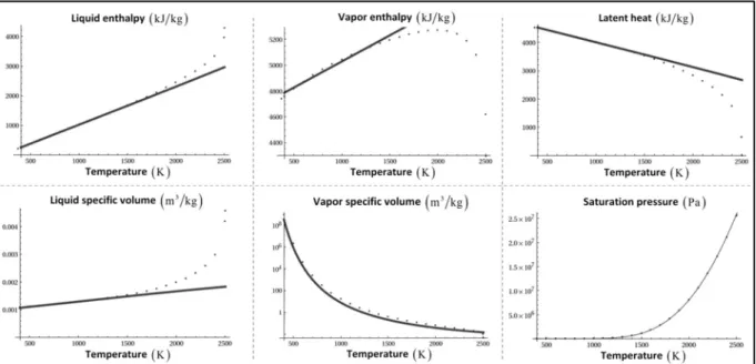
Parameters of liquid water and its vapor are given in Le Metayer and Saurel (2016). Regarding sodium, saturation curves are given in Fink and Leibowitz (1995) and the various EOS parameters (vapor and liquid) are determined from these data. The corresponding theoretical curves are compared to the reference ones in Figure 3.1.

The soda heat capacity at constant pressure ( L _a p,N OH

c 2100 J kg K) is taken constant and adjusted at T 1000 K from Chase (1998). The liquid soda density as a function of temperature at atmospheric pressure is given in Daubert et al. (1994) and leads to the determination of parameters L _a

v,N OH c , L_a N OH b and L _a ,N OH p . The value of a L N OH  is then obtained as L _a L_a L _a p,N OH N OH v,N OH

c   c . Finally, it should be noted that the liquid soda reference energy L_a

N OH

q is determined to agree with the surface reaction heat release, as detailed in Section 4.

8

Figure 3.1: Reference (points) and theoretical (lines) sodium saturation curves. Very good agreement is observed in the temperature range



300K 1500K



. This range is wide enough for SWR studies as explosions typically occur when the

sodium temperature reaches about 1000K (Daudin, 2015).

3.2. Mixture equation of state

From System (3.1) and having in hands the NASG EOS for each phases and fluids, two relationships enable mixture temperature computation. From the mixture specific volume definition

 

N k k k 1 v Y v p,T 





, the mixture temperature is obtained as:

 

_

_

N k k k 1 N k v,k k k 1 ,k v Y b T p,v Y c 1 p p        





. (3.2)

From the mixture internal energy definition N k k

 

k 1

e Y e p,T 





another relation for the mixture temperature is obtained:

 

_

_

N k k k 1 N N k v,k k ,k k v,k k 1 k 1 ,k e Y q T p,e Y c 1 p Y c p p           







. (3.3)

Combining these two relations the mixture pressure becomes solution of the equation f p

 

0 with,

 





N k k N N k v,k k k 1 ,k k v,k N k 1 ,k k 1 k k k 1 e Y q Y c 1 f p p Y c p p _{v Y b}        _             _     









. (3.4)

Its resolution requires an iterative method such as Newton’s one.

The thermodynamic closure of System (2.1) being determined we now address modeling of the various chemical reactions.

4. Chemical reactions

System (2.1) involves both gas phase reactions through production terms GR and surface reactions

9

4.1 Surface reaction

Water vapor is produced at the liquid-gas interface and diffused through the gas layer to the sodium surface. As molecular diffusion is a slow process compared to the kinetics of the surface reaction, this one is considered instantaneous. A single global reaction between liquid sodium and water vapor is considered:  L  v  L  g a 2 a 2 1 N H O N OH H 2    . (4.1)

This reaction is exothermic,

0 SR

H 177kJ / mol

   .

Reaction (4.1) is expressed in mass terms:

 L 2  v a  L 2  g a 2 a 2 a a a N OH H O H N H O N OH H N N N W W W 1kg kg kg kg W W 2W    , i.e.,  L ₂  v _a  L ₂  g a H O 2 N OH a H 2 N H O N O H H 1kg   kg   kg   kg , with H O₂ 0.78, N OH_a 1.74 and  H₂ 0.04.

As this reaction is instantaneous its numerical treatment is easy. The liquid sodium and water vapor are compared first:

- If the water vapor concentration is limiting



g_{2 2} L_a



H O H O N

Y Y

    , then the mass increment is computed as, 2 2 g H O SR H O Y d   . - Otherwise L_a SR N d  . Y

The various mass fractions are then updated as,

 

a a * L L N N SR Y Y d     



2



2 2 * g g H O H O H O SR Y Y d      



a



a a * L L N OH N OH N OH SR Y Y d      

 

2 2 2 * g g H H H SR Y Y d       ,

the state ‘*’ being the post-reaction one.

Agreement with the surface reaction



0 _a



SR N

H 177kJ/mol 7.702MJ/kg

     heat release is achieved by

adjusting the reference energy of liquid soda as detailed hereafter.

Each phase is governed by the NASG equation of state with the enthalpy defined as,

 

k p,k k k h p,T c T b p q  , where constants g₂ H O b and g₂ H b are zero.

With this definition the heat of reaction at atmospheric conditions



p ,T0 0



reads,  



L





 g





 g





 L



a _a a a 2 ₂ 2 2 ₂ 2 _a a a a 0 L L g g L L SR N OH _{p,N OH} 0 N OH 0 N OH H _p,H 0 H H O _{p,H O} 0 H O _p,N 0 N 0 N N H c T b p q c T q c T q c T b p q 7.702MJ / kg                

The reference energy of hydrogen is zero

_

g₂

_

H

q 0 . Those of both liquid sodium and water vapor

have been determined in Section 3.1 to agree with the latent heats of vaporization. The reference energy of liquid soda is consequently determined to respect 0

SR H  :        



L g g L



a a _a 2 ₂ 2 _{2 a} a a a 2 2 a a a L L g L N N OH _{p,N OH} H _p,H H O _{p,H O p,N} 0 N OH N OH 0 N 0 H O H O N L N OH N OH 6 7.702MJ / kg c c c c T b p b p q q q 3.974 10 J / kg                   

10

This data corresponds to the one reported in Table 3.1. 4.2 Gas phase reaction

A single global gas reaction is considered between water vapor and sodium vapor. It produces liquid soda and gas hydrogen:

 v  v  L  g a 2 a 2 1 N H O N OH H 2    (4.2)

The associated heat release is, 0 GR

H 281kJ / mol

   .

This reaction is considered instantaneous as before. Few details on the kinetics of this reaction are available (Takata and Yamaguchi, 2003). At this level it is assumed that this reaction is very fast compared to the other physical processes in presence, such as mass diffusion. This assumption will be reconsidered in Section 10.

Numerical treatment of this reaction follows the same lines as the previous one: - If the water vapor concentration is limiting



g_{2 2} g_a



H O H O N Y Y     , then 2 2 g H O GR H O Y d   , - Otherwise, g_a GR N d   . Y

The various mass fractions are then updated as,

 

a a * g g N N GR Y Y d     



2



2 2 * g g H O H O H O GR Y Y d      



a



a a * L L N OH N OH N OH GR Y Y d      

 

2 2 2 * g g H H H GR Y Y d       ,

the state ‘*’ being the post-reaction one.

The flow model (2.1) with thermodynamic closure (3.4), complemented by mass transfer treatment given in Appendix B and chemical production rates given by equations (4.1) and (4.2) form a closed system of equations. Its numerical resolution poses many challenges that are addressed gradually, the first one being related to the capture of interfaces and associated numerical diffusion.

5. Interface sharpening

In this section, System (2.1) is considered in the absence of heat and mass diffusion, capillary effects and source terms. It thus reduces to the hyperbolic part of the model with thermodynamic closure (3.4). Its numerical resolution is achieved in the DALPHADT© code based on both structured and unstructured meshes [www.rs2n.eu]. The Riemann solver used to compute the intercell flux is the HLLC one (Toro et al., 1994), see Saurel et al. (2016) for adaptation to the present flow model. MUSCL type reconstruction is used, as detailed in Chiapolino et al. (2017) for unstructured grids. As detailed in this reference a well-known issue appears during the simple transport of an interface. Numerical diffusion smears interfaces over several points even when compressive limiters, such as Superbee (Roe, 1985) are used. To overcome this difficulty the Overbee limiter of Chiapolino et al. (2017) is used. It consists in a compressive limiter valid for linearly degenerate fields only and transport of Heaviside function, such as volume fraction separating two fluids.

The method is adapted to the flow model (2.1) by adding extra equations with respect to the volume fractions, k k u. 0 t  _{  }    , (5.1)

where k represents : liquid water

 

H O , liquid sodium 2 L

 

N , liquid soda a L



N OH , multi-component a



L

11

The Overbee limiter is used for these equations only. Denoting by _f the ratio of two gradients adjacent to a cell face (   f



i 1 i

 

  in the simplified case of structured mesh), i i 1



extrapolation from the cell center to the face is done through limited gradients through the formula:  f m ax 0 ,m in 2 ,2 f 

   _  _.

This limiter is used at interfaces only, that are detected as,

n n k j

   , with j k .

According to numerical experiments, _{ 10}2 _{seems a fair choice.}

The other flow variables present in System (2.1) are computed with the same method, except that the Minmod limiter is used.

System (5.1) is solved during each time step of the hyperbolic solver. Sharpening volume fractions with the help of Overbee limiter results in enhanced accuracy in the various fluxes computation and consequently in sharpened mixture density and mass fractions.

But adding System (5.1) to System (2.1) corresponds to an overdetermined system. At the end of the time step all variables must be compatible and this is done through the reset of the various volume fractions. With the help of the computed equilibrium pressure p_eq and temperature T_eq given by (3.4) and (3.3), based on mass fractions (and not volume fractions) the volume fractions are reset as: -For liquids,



k



k k eq eq Y , k 3 p ,T       .

-For the multicomponent gas mixture (made of 4 species):





7 k g k 4 k eq eq Y p ,T     



.

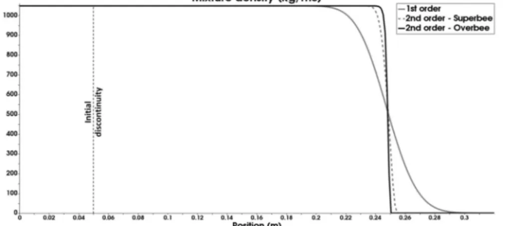
The method is illustrated on the advection test of Figure 5.1 with data relevant to SWR situations. Let us consider a 1D 32cm long tube with an interface separating two fluids (nearly pure liquid water on the left, nearly pure air on the right). The flow variables are uniform in the whole domain,

0 0 0 u 0.1m / s p 0.1MPa T 300K         ,

except the mass and volume fractions, as well as mixture density that are discontinuous at x=0.05 m at initial time. Three computations are compared at the same time in Figure 5.1. The accuracy gain observed on the interface capture is noticeable with Overbee.

Figure 5.1: Comparison between Superbee and Overbee limiters for the advection of a liquid-gas interface at low speed – Mesh: 240 cells – CFL=0.8 – Final time: 1.98s. As the CFL is based on the sound speed more than 3 600 000-time steps are

required to reach final time.

Another difficulty is now addressed and is related to the numerical treatment of mass diffusion with numerically diffuse interfaces. Indeed, even if the Overbee limiter reduces numerical diffusion, interfaces are still diffused and need special care when physical mass diffusion is considered.

12

6. Mass diffusion with diffuse interfaces and effects of chemical reactions

To illustrate the difficulty let us consider a 1D configuration relevant to SWR. A spherical liquid drop of 1mm radius is set in liquid water. The two liquids are separated by a 2 mm gas layer at elevated initial temperature. A schematic representation of the configuration under interest is shown in Figure 6.1.

Figure 6.1: 1D configuration relevant to typical SWR situations with a 1 mm radius sodium droplet separated by a gas layer from liquid water. The liquid water domain boundary is treated as an inflow/outflow boundary condition. Precisely liquid

water tank at atmospheric pressure and temperature 373 K is imposed at outflow. This outflow may become an inflow if the flow becomes inverted. Details are given in Appendix C.

For a first run, mass diffusion is removed as well as chemical reactions, both in the gas phase and at sodium surface. Surface tension and gravity effects are obviously absent. Therefore, only fluid motion is considered in the presence of heat conduction and phase transition of both water and sodium. Corresponding results are shown in Figure 6.2.

Figure 6.2: 1D reference results related to the 1D SWR test problem of Figure 6.1. Computed results are shown at time 15 ms on a mesh involving 150 cells. Thermal diffusion and phase transition only are present in the flow model (2.1). From the initial situation the gas layer has been cooled and water vapor appears at the interface at right. Both interface motions have

been considered but their velocity is not significant in the present example.

In the second run, mass diffusion within the gas phase is considered with constant mass diffusion coefficient: _{C 10 kg m s} 4 _{. Corresponding results are shown in Figure 6.3 at time 15ms (same as}

before). The water vapor created at the gas-liquid water interface is now diffused within the multi-component gas until it reaches the liquid sodium-gas interface.

13

Figure 6.3: 1D computed results related to the 1D SWR test problem of Figure 6.1 in the presence of mass diffusion in addition to fluid motion, heat diffusion and phase transition already considered in the results of Figure 6.2. Same mesh is

considered, and the results are shown at the same time. The gas-liquid water interface becomes corrupted as a consequence of mass diffusion in the numerically diffuse interface.

The interface separating the gas mixture and liquid water becomes unphysical, as clearly visible on the mixture density and volume fraction graphs. This issue results of bad interaction between the mass diffusion flux and the diffuse interface representation.

In the frame of diffuse interface methods, a ‘pure’ liquid is numerically treated as a mixture with a liquid volume fraction equal to 1. The other fluids in minor proportion then share the residue . This remark also holds for the related mass and molar fractions. In liquid water, the multi-component gas mass fraction, and in particular the water vapor one, are therefore zero. This implies a non-zero water vapor molar fraction (although physically inconsistent) in the liquid water domain. Computation of the related gradient 

2

H O

x present in the mass diffusion flux is consequently wrong. Weighting the related mass diffusion flux by the gas volume fraction, as done in System (2.1) through the term  g₂

g H OF is not enough to cure this problem.

To circumvent this difficulty the mass diffusion coefficient C is rendered dependent to the liquid water mass fraction as follows:

 

2

 

2 L L H O 0 H O C Y C H Y , (6.1) with 4 0 C _10 kg m s _,

 

2 2 2 L H O L H O L H O 1, if Y 0.5 H Y 0, if Y 0.5         _{  }

 and  



0.5;0.5



a parameter to define.

Function

_{ }

2

L H O

14

Figure 6.4: Function

 

2

L H O

H Y used in the mass diffusion coefficient correction.

Function

_{ }

2

L H O

H Y prevents mass diffusion in quasi-pure liquid zones and prevents interface

corruption.

_{ }

L₂ H O

H Y is used only at the gas-liquid water interface. Indeed, at the sodium-gas

interface the presence of surface reaction prevents such defect.

With the help of this non-linear diffusion coefficient, the 1D spherical test of Figure 6.1 is rerun. Parameter  is set to  0.2. Results are shown at the same time as before (15ms) in Figure 6.5, showing correct interface behavior.

Figure 6.5: 1D computed results related to the 1D SWR test problem of Figure 6.1 in the presence of mass diffusion with non-linear mass diffusion coefficient (6.1). Fluid motion, heat diffusion, phase transition and mass diffusion are considered

on the same mesh as in the previous computations, with 150 cells. Sharp liquid water - gas mixture interface is now recovered and mass diffusion in the gas phase is present. Mass diffusion effects appear clearly by comparing the mass

fraction graphs of the present figure and the one of Figure 6.2.

Influence of the parameter 

The 1D spherical test of Figure 6.1 is rerun for different values of parameter  in order to assess its influence on the numerical results. For each test the water vapor mass fraction at the gas-liquid water interface is recorded at different times and shown in Figure 6.6. Influence of parameter  in the range



0.2;0.2



appears not noticeable.

15

Figure 6.6: The 1D SWR test problem of Figure 6.1 is considered in the presence of fluid motion, heat diffusion, phase transition and mass diffusion. Results obtained with 3 different values of parameter  are compared. The quantity of water vapor produced at the interface does not depend on the parameter  in the range



0.2;0.2



. Outside this range,

differences appear.

The interfacial water vapor mass fraction does not depend on the parameter  in the range



0.2;0.2



at least in the present configuration. This parameter is set to   0.2 in the following.

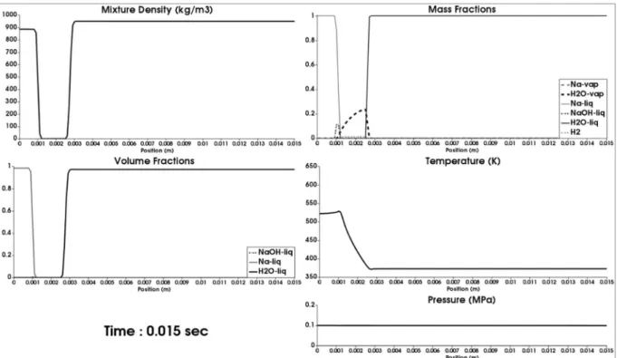
As water vapor now diffuses from the liquid water side to the sodium one it becomes possible to address both surface and volume reactions. To this end the various production terms addressed in Section 4 are used. Computed results are shown at the same time as before, on the same mesh and are shown in Figure 6.7.

Figure 6.7: 1D computed results related to the 1D SWR test problem of Figure 6.1 in the presence of both surface and gas reactions. Fluid motion, heat diffusion, phase transition, mass diffusion



with 0.2



and chemical reactions are considered on the same mesh as in the previous computations, with 150 cells. Results are shown at the same time as before (15ms). The liquid sodium temperature increases, compared to the results of Figure 6.5, as a consequence of surface

reaction combined to heat diffusion.

When the water vapor reaches the liquid sodium-gas interface, surface reaction occurs, generating large soda mass production and local heating. It contributes to both liquid sodium and gas film heating through thermal diffusion. At this level, the interface motion is still imperceptible.

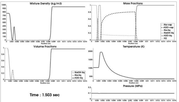
Results at longer times are shown in Figures 6.8 (t=1.503s) and 6.9 (t=2.334s). At time 1.503s, the liquid sodium temperature exceeds 1000K. At this temperature, a larger amount of sodium vapor is produced. This vapor then reacts with the water one through the gas reaction. The gas reaction being

16

more exothermic than the surface one, the temperature locally exceeds 1800K. The mass fraction of the produced liquid soda is locally close to 1 and acts as a barrier between sodium and water vapors present in large quantities. The SWR gas product (hydrogen H₂) is diffused within the gas layer. In addition, the gas film thickness has significantly increased, compared to the one observed in Figure 6.7, at time t=15ms.

Figure 6.8: 1D computed results related to the 1D SWR test problem of Figure 6.1 in the presence of fluid motion, heat diffusion, phase transition, mass diffusion



 0.2



and both surface and gas reactions. The mesh made of 150 cells is still

considered. Results are shown at time t=1.503s. At this stage, the gas film thickness has considerably increased. The liquid sodium temperature exceeds 1000K. The liquid soda film separates both sodium and water vapors present in large

proportions.

Figure 6.9: 1D computed results related to the 1D SWR test problem of Figure 6.1 in the presence of fluid motion, heat diffusion, phase transition, mass diffusion



 0.2



and both surface and gas reactions. The mesh made of 150 cells is considered again. Results are shown at time t=2.334s. At this stage, the sodium has been fully consumed. A hot (about

17

At time 2.334s (Figure 6.9), liquid sodium has exceeded boiling point (1156K at atmospheric pressure) and sodium vapor has been fully consumed. It results in hot



2000K



soda drop formation. The gas film continues to grow, while the soda drop gradually cools. No explosion (with shock wave emission) is observed. The pressure is nearly uniform in the Figures 6.2 to 6.9.

Three main points emerge of the former 1D numerical experiments:

- The diffuse interface model is able to model at least qualitatively the complex physics present in SWR process;

- The combustion regime observed in these tests is governed by thermal and mass diffusion. As the distance increases monotonically versus time the various gradients and associated fluxes decrease forbidding explosion occurrence;

- A liquid soda layer appears close to the sodium surface, lowering gas mass diffusion from the liquid water surface.

These observations motivate multi-D modelling, as illustrated in Figure 6.10. Indeed, the gas layer width is selected as a consequence of the various diffusive and reactive effects, in competition with gas ejection at the free surface and weight of the sodium drop. Also, gas ejection has potential to remove liquid soda layer. Multi-D effects are expected to maintain intense gradients oppositely to 1D computations. However, two main numerical issues appear in addition to those already addressed in Sections 5 and 6. These issues are related to body and surface forces and are addressed in the forthcoming sections.

Figure 6.10: Schematic representation of the motivations for 2D computations. The gas layer width is selected by the competition of heat and mass diffusion, phase transition, exothermicity of the various reactions against gas ejection and

weight of the sodium drop.

7. Numerical approximation of gravity effects

Accurate computation of gravity effects is of primary importance in the present context as gas layer width selection, directly linked to the various diffusive effects present in the flame, is closely driven by buoyancy.

System (2.1) involves gravity through source terms present in both mixture momentum and mixture energy balance equations. Source term splitting methods are well known to produce instabilities, particularly when dense fluids are considered. Insertion of gravity effects in the flux computation, through ‘well balanced’ Riemann solvers has been the subject of many efforts, such as for example LeVeque (1998), Gosse (2000) and Gallice (2002).

In the present section the HLLC solver (Toro et al., 1994) is considered and gravity effects are embedded in the formulation. This solver is genuinely positive, an important property when dealing

18

with material interfaces and large density ratios, as well as sophisticated EOS, as the one given in Section 3.

Let us consider the hyperbolic part of System (2.1):

 

U _{div F 0} t  _{ }  , (7.2) with k Y U u E       _{ } _     and





k Y u F u u pI E p u                        .

In the HLLC solver framework, three waves are considered:

- The extreme waves speeds SL and SR, estimated as (Davis, 1988),

 

 





L f _L L f _R R S min u.  c , u.  c

 

 





R f _L L f _R R S max u.  c , u.  c , with f 

the unit normal vector of the face f oriented towards the cell R. For the sake of simplicity, normal velocities are denoted by

 

u.f _L uL

 

and

 

u.f _R uR

 

in the following. - The contact discontinuity speed SM , to determine in the presence of gravity effects.

The Rankine-Hugoniot relations through the extreme waves read,

   

*



_*



f _L f _L L L L

F.  F. S U U ,

   

*



*



f _R f _R R R R

F.  F. S U U (7.3)

and lead, in particular, to the usual expressions of pressure in the star regions:







* L L L L L L M p p   u S u S , *







R R R R R R M p p   u S u S (7.4)

In the framework of the standard HLLC solver without gravity effects, the pressure equality is ensured through the contact wave ( * *

L R

p p ). But in the present context, the determination of the contact condition requires the integration of the equilibrium condition:

p g

    

,

with





T

g 0 g the gravity vector.

The equilibrium condition can be rewritten as follows:

p ₀ x p _g y   _       _{ }    (7.5) Integration of the second relation is achieved on both sides of face f separating the two cells L and R:

R R * p y * R R R R y p dp  gdyp   gy p   gy





, * L L p y * L L L L p y dp  gdyp  gy p  gy





(7.6)

with _p* _{the pressure solution of the Riemann problem and y the vertical coordinate of the center of}

face f (Figure 7.1).

Relations (7.6) can be rewritten in the star states as follows:

* * R R R R * * L L L L p gy p gy p gy p gy               , (7.7)

where the density variations have been assumed to be negligible through the acoustic waves.

Combining (7.4) and (7.7) leads to the determination of both contact wave speed SM and star

pressure _p*_:    









     





 



 



       





 





    R L L L L L R R R R R R L L M L L L R R R L L L R R R R R L L R R R R R L L L L L L L L R R R * L L L R R R L L L R R R p p u S u u S u g y y g y y S S u S u u S g y y u S g y y p u S u u S p u S u u S p u S u S u S u S  _{           }  _                                 _{         }  (7.8)

19

Figure 7.1: Determination of y for two mesh types (triangular and cartesian grids). PL and PR represent respectively the

centers of cells L and R. P_f is the center of the face f.

The primitive variable vector in the star states is thus fully determined and the solution sampling is done to compute the flux F of System (7.2).

For example, in the subsonic case such as SM0, the flux solution of the Riemann problem on a

given face f along the face normal vector f

 reads,

 





* * L k,L M * _{* * *} f L M L f * * * L L M Y S F. S u p E p S                        , with





* k,L k,L * L L L L M L * * L L M L L L L L * L M f L Y Y u S S S p u p S E E u S u S u         _   _               .

In these formulas, u _L_{  }u u_{L L f} _{denotes the velocity vector tangential to the face f. Moreover,}

M

S

and _p* _{are defined by (7.8). The use of p}* _{instead of} * L

p and * R

p given by (7.4) is a consequence of the pressure profile linearity, characteristic of gravity effects. Let us consider the specific case of a state close to the equilibrium one. Any small velocity fluctuation modifying the sign of SM would lead

to an unacceptable variations between * L

p and * R

p if the latter was chosen to compute the flux _F*_.

The choice of _p* _{therefore allows to preserve the mechanical equilibrium condition.}

In the supersonic case such as S 0L , the solution reads:

 





L k,L L * _* f L L L f * L L L Y u F. u u p E p u               _{ }       , with *





L L L p p  g y y .

The following Godunov type scheme is then used to update the solution. For the sake of simplicity its formulation is given hereafter at first order,

 

Faces N _* n 1 n n i i f f i f 1 i t U U F. L tH S     



   , with k Y U u E       _{ } _     ,





k Y u F u u pI E p u                        and 0 H g g.u      _{ } _       . f

L denotes the length of the face f, Si is the surface of the cell i and NFaces represents the number of

faces of the considered cell. The superscripts n and n+1 denote two successive time steps _tn _{and t}n 1

20

Efficiency of this method is illustrated on the following test case. Let’s consider a 10m height tank, the lower half tank being filled with water and the upper one with air. The initial pressure in the entire vessel is the atmospheric one. The considered mesh is coarse (100 cells) to highlight differences between the conventional splitting method and the present one, where gravity effects are embedded in the Riemann solver. Corresponding results are shown in the Figure 7.2.

Figure 7.2: Mechanical equilibrium of a water column in air. The conventional Godunov method with source terms splitting is compared to the present one, where gravity terms are embedded in the HLLC solver. Both methods compute correct pressure field, but the new method only is free of parasitic velocity when equilibrium is reached. Computed results are

shown at time 3 s.

The equilibrium state is perfectly matched with the new method. We now address surface tension effects approximation with similar approach.

8. Numerical approximation of surface tension

Surface tension effects are considered through the Continuum Surface Force (CSF) method of Brackbill et al. (1992). The capillary force is modelled as:

liq

F_ ,

where  represents the surface tension coefficient, _liq is the liquid volume fraction and 

represents the local curvature

_{ }

_m1 :

liq liq div     _      (8.1)

In system (2.1) these effects are present through the term (        a a a 2 2 2

L L

N N N H O H O H O) in the

momentum and energy equations. Two contributions are present as two interfaces are considered. The CSF method has been already considered with compressible fluids and diffuse interfaces (Perigaud and Saurel, 2005, Le Martelot et al., 2014, Garrick et al. 2017, Schmidmayer et al., 2017) but extra difficulties appear in the present application as a result of interface sharpening through the method presented in Section 5. Computation of the local curvature becomes problematic. The approach used in the present work is described gradually in the following.

8.1 Volume fraction gradient determination at cell centers

A robust and accurate method for the computation of the volume fraction gradient is based on least squares approximation. It is based on multiple Taylor expansions around cell center Pi and a cloud of

21

 

 

2 i i j i i j x i j y i j 2 i i i ij ij i j PP .e PP .e PP x y x y PP x y                              , (8.2) where ex  and ey 

denote the unit vectors of the Cartesian basis.

Using (8.2) with a set of N neighbors



j1 ,...,N



results in the following system:









1 i1 1 i1 1 1 i i i N iN N iN N N i x y . . . x . . . AX B . . _y . x y                       _                     _{  } _{   }  _{   }      , with _{j 2 2} ij ij 1 x y      .

Weights j allows to control numerical instabilities (division by small numbers) when the mesh is

skewed. In two dimensions, a minimum of two neighboring elements is necessary to solve the system. When the number of available neighbors is greater than two, then the system is over-determined. A classical way to solve this over-determined system is to multiply both sides of AX B

by the transpose matrix. A square system is obtained: _{A AX A B}T _ T _{, and the solution reads,}

 

_T 1 _T

X A A A B .

It is possible to consider direct neighbors only of the considered cell (direct stencil) or both direct and indirect neighbors (extended stencil). Both configurations are schematized in Figure 8.1.

Figure 8.1: Schematic representation of the direct and indirect neighbors of the considered cell on an unstructured mesh made of triangles. On the left, only the direct neighbors are colored (direct stencil). On the

right, both direct and indirect neighbors are colored (extended stencil).

In the following, extended stencil is retained for accuracy reasons. The liquid volume fraction gradient being determined, the next step consists in computing the interface curvature at each cell center.

8.2 Interface curvature determination at cell centers

The local curvature has been defined in (8.1) and requires volume fraction gradients computation, as detailed earlier. However, as the liquid volume fraction has been sharpened with the method given in Section 5 difficulties emerge. The liquid volume fraction gradient is not defined in a sufficiently wide stencil to compute curvature accurately.

To circumvent this difficulty, a color function Cliq with smooth profile is introduced. It is built at each

time step with the following initial data,

liq liq liq If 0.5, C 1 Otherwise, C 0      _ 

22

Neigh Neigh N n n i liq,i k liq,k n 1 k 1 liq,i N i k k 1 S C S C C S S      





,

with N_Neigh the number of direct neighbors of the cell i and Si the surface of the cell i.

Using this operator during 5 iterations results in a diffuse profile on approximatively 5 cells. The corresponding color function is shown in Figure 8.2 in the specific case of a 2D liquid drop.

Figure 8.2: Color function representing a liquid drop surrounded by air on an unstructured mesh.

The diffused color function is therefore a good candidate for curvature calculation. The latter is then computed as: liq liq C div C _       _      .

In two-dimension the local interface curvature at a cell center i reads,

2 2 2 2 2

liq,i liq,i liq,i liq,i liq,i liq,i liq,i

2 2 i 3 liq,i C C C C C C C 2 x y x y x y y x C               _  _{    }  _  _         . (8.3)

This expression involves color function gradient components at cell centers, as well as color function Hessian matrix components. Computation of these terms is achieved with the help of the least-squares method detailed in Section 8.1 and used twice. First with the cell center color function as argument and second with resulting gradient components that become arguments of the Hessian matrix approximation.

Curvature computation oscillations

To validate the curvature computation method, a test with a simple circular interface is considered. By definition it is the inverse of the radius. Let us consider a 5mm radius sodium drop with curvature 200_m1_.

The curvature obtained using (8.3) is shown in Figure 8.3, for two types of meshes (triangular cells and square ones). Whatever the mesh used, the computed curvature oscillates along the interface. It is thus necessary to correct its computation. This issue has been reported many times (Renardy and Renardy 2002, Garrick et al. 2017)

23

Figure 8.3: Computed curvature for a circular interface – Two types of meshes are considered – Only cells with curvature close to the theoretical value are shown. Large variations are present.

Curvature correction

Curvature computation is accurate at cells located on the interface, i.e. at cells for which the color function is close to 0.5. The method adopted consists in extending the value of the curvature computed in these cells to the surrounding ones, with the help of a weighted diffusion operator (Garrick et al., 2017). This is done with the following iterative method, used at each time step,

Neigh Neigh N n n i i k k n 1 k 1 i N i k k 1             





, with

_

_

2 k S Ck liq,k 1 Cliq,k 

  _  _ a Gaussian weighting function centered on the interface where Cliq ,k 0.5.

This correction is illustrated in Figure 8.4 with the same 5 mm radius sodium drop test case as before.

Figure 8.4: The circle curvature is computed with the two different types of meshes (triangles on top, squares on bottom). For each mesh type, varying numbers of iterations in the curvature diffusion method are used.

Accuracy of the curvature computation increases with the number of iterations of the diffusion method. However, we note that the convergence towards the theoretical value is faster in the case of square cells. However, it is important to limit corrections, especially in zones where the interface is highly curved, as neighboring cells values would corrupt the correct value of . In the various computations that will be presented in Section 9, Cartesian grids are used with typically 10 iterations. In the present application smooth interfaces are mainly considered and the method appears appropriate. To preserve mechanical equilibrium extra ingredient is needed such as specific Riemann solver, as examined hereafter.

24

8.3. Capillary HLLC Riemann solver

In order to avoid numerical errors due to operator splitting, surface tension has to be taken into account in the Riemann solver. The same arguments as those associated to gravity effects hold. Building HLLC-type Riemann solver including capillary effects follows the same lines as the one with gravity. Let us consider the hyperbolic part of System (2.1), in the simplified context of a mixture made of a single liquid and a gas. The Rankine-Hugoniot relations (7.3) through the extreme waves of speeds SL and SR (estimated as done in Section 7) are used again. The same expressions of star

pressures given by (7.4) are recovered. Indeed, surface tension has effects only at contact waves, not across acoustic ones.

In the presence of surface tension pressure equality through the contact wave ( * * L R

p p ) is replaced by the following condition (Perigaud and Saurel, 2005, Garrick et al., 2017):





* * R L liq,R liq,L p p      , with  L R 1 2      .

As the curvature as been smoothed in a band surrounding the interface, the simple average above has been found appropriate to estimate the curvature at cell boundaries.

The contact relation is in agreement with the Laplace law. Typical examples and verifications are illustrated in Figure 8.5.

Figure 8.5: The various configurations that may occur at a curved interface separating a liquid and a gas.

The star pressure _p* _{is then obtained as:}

* * *

R liq,R L liq,L

p p   p   (8.4)

Combining (7.4) and (8.4) implies:





































































R L L L L L R R R R liq,R liq,L M L L L R R R R R R R R L L L L L L L L R R R liq,R L L L liq,L R R R * L L L R R R L L L R R R p p u S u u S u S S u S u p u S u u S p u S u u S u S u S p u S u S u S u S                                          _{  }  _{         }  (8.5) The first relation of System (8.5) corresponds to the one given in Garrick et al. (2017). The primitive variable vector in the star states is thus fully determined and the solution sampling is done to compute the flux F.