HAL Id: hal-00330811
https://hal.archives-ouvertes.fr/hal-00330811
Submitted on 20 Nov 2007HAL is a multi-disciplinary open access
archive for the deposit and dissemination of sci-entific research documents, whether they are pub-lished or not. The documents may come from teaching and research institutions in France or abroad, or from public or private research centers.
L’archive ouverte pluridisciplinaire HAL, est destinée au dépôt et à la diffusion de documents scientifiques de niveau recherche, publiés ou non, émanant des établissements d’enseignement et de recherche français ou étrangers, des laboratoires publics ou privés.
On the measurement of solute concentrations in 2-D
flow tank experiments
M. Konz, P. Ackerer, E. Meier, P. Huggenberger, E. Zechner, D. Gechter
To cite this version:
M. Konz, P. Ackerer, E. Meier, P. Huggenberger, E. Zechner, et al.. On the measurement of solute concentrations in 2-D flow tank experiments. Hydrology and Earth System Sciences Discussions, European Geosciences Union, 2007, 4 (6), pp.4175-4210. �hal-00330811�
HESSD
4, 4175–4210, 2007 Concentration determination on flow tank experiments M. Konz et al. Title Page Abstract Introduction Conclusions References Tables Figures ◭ ◮ ◭ ◮ Back CloseFull Screen / Esc
Printer-friendly Version Interactive Discussion
EGU
Hydrol. Earth Syst. Sci. Discuss., 4, 4175–4210, 2007 www.hydrol-earth-syst-sci-discuss.net/4/4175/2007/ © Author(s) 2007. This work is licensed
under a Creative Commons License.
Hydrology and Earth System Sciences Discussions
Papers published in Hydrology and Earth System Sciences Discussions are under open-access review for the journal Hydrology and Earth System Sciences
On the measurement of solute
concentrations in 2-D flow tank
experiments
M. Konz1, P. Ackerer2, E. Meier3, P. Huggenberger1, E. Zechner1, and D. Gechter1
1
University of Basel, Institut of Geology, Applied Geology, Switzerland
2
Universit ´e Louis Pasteur, Institut de M ´ecanique des Fluides et des Solides, CNRS, UMR 7507, France
3
Edi Meier & Partner AG, Winterthur, Switzerland
Received: 30 October 2007 – Accepted: 30 October 2007 – Published: 20 November 2007 Correspondence to: M. Konz ([email protected])
HESSD
4, 4175–4210, 2007 Concentration determination on flow tank experiments M. Konz et al. Title Page Abstract Introduction Conclusions References Tables Figures ◭ ◮ ◭ ◮ Back CloseFull Screen / Esc
Printer-friendly Version Interactive Discussion
EGU
Abstract
In this study we describe and compare photometric and resistivity measurement methodologies to determine solute concentrations in porous media flow tank exper-iments. The first method is the photometric method, which directly relates digitally measured intensities of a tracer dye to concentrations without previously converting
5
the intensities to optical densities. This enables an effective processing of a large amount of images to compute concentration time series at various points of the flow tank. Perturbations of the measurements are investigated and both lens flare effects and the image resolution turned out to be the major sources of error. An attached mask is able to minimize the lens flare effects. The second method for in situ
measure-10
ment of salt concentrations in porous media experiments is the resistivity method. The resistivity measurement system uses two different input voltages at gilded electrode sticks to enable the measurement of salt concentrations from 0 to 300 g/l. Power laws are used to relate apparent resistivity values and salt concentrations. However, due to the unknown measurement volume of the electrodes, we consider the image analysis
15
method more appropriate for intermediate scale laboratory benchmark experiments to evaluate numerical codes.
1 Introduction
The modelling of density driven flow in porous media is still a challenge (Diersch and Kolditz, 2002; Hassanizadeh and Leijnse, 1995) and mathematical models and
numer-20
ical codes have been tested and evaluated in details. Laboratory experiments are an excellent way of providing data to assess or not new theories and validate or not numer-ical codes. They have several advantages: boundary and initial conditions are known, the porous medium properties can be defined separately and the experiments can be repeated if necessary. Excellent reviews mass transfer in porous media at the
labora-25
HESSD
4, 4175–4210, 2007 Concentration determination on flow tank experiments M. Konz et al. Title Page Abstract Introduction Conclusions References Tables Figures ◭ ◮ ◭ ◮ Back CloseFull Screen / Esc
Printer-friendly Version Interactive Discussion
EGU
methods exist for qualitative and quantitative determination of solute transport in experi-mental porous media at that scale. Traditionally this is done by intrusive methods where extracted fluids are analysed in the laboratory (e.g. Swartz and Schwartz, 1998; Barth et al., 2001). These methods are work intensive and require a well-equipped labora-tory for chemical analysis. Further, the temporal and spatial resolution of concentration
5
determination is limited due to point sampling and perturbations of the flow field cannot be excluded. Oostrom et al. (2003) introduced the non-intrusive dual-energy gamma radiation system methods for 3-D experiments. Oswald et al. (1997) and Oswald and Kinzelbach (2004) used nuclear magnetic resonance (NMR) technique to derive con-centration distributions of 3-D benchmark experiments for density dependent flow. This
10
method is very precise but it is limited to small flow tank experiments due to the size of the NMR tomograph.
In the published literature dyes have been mainly used to qualitatively and quan-titatively visualize spatial mixing patterns of contaminants in 2-D porous media flow tank experiments (Oostrom et al., 1992, Schincariol et al., 1993, Schwartz and Swartz,
15
1998, Wildenschild and Jensen, 1999, Simmons et al., 2002, Rahman et al., 2005, Mc-Neil et al., 2006, Goswami and Clement, 2007). The dye itself was used as contaminant (e.g. Rahman et al., 2005) or it acts as optical tracer to mark contaminants with den-sity effects (e.g. Schincariol et al., 1993, McNeil et al., 2006, Goswami and Clement, 2007). Schincariol et al. (1993) and McNeil et al. (2006) relate optical densities to
20
concentrations of dye tracer. This involves (i) the optimization of intensity vs. optical density standard curve of each image to be investigated and (ii) an optimization of opti-cal density vs. concentration standard curve. If only the spatial evolution of plumes at a limited number of time-steps is investigated the computational efficiency is of minor im-portance because the intensity vs. optical density standard curve has to be optimized
25
only for a little number of images. For the evaluation of numerical codes however, breakthrough curves at distinct points with a high temporal resolution are necessary. This requires processing of a large number of images and the computational efficiency becomes a significant criteria.
HESSD
4, 4175–4210, 2007 Concentration determination on flow tank experiments M. Konz et al. Title Page Abstract Introduction Conclusions References Tables Figures ◭ ◮ ◭ ◮ Back CloseFull Screen / Esc
Printer-friendly Version Interactive Discussion
EGU
In this study we present an optical and a resitivity based approach to measure salt concentrations of a wide concentration range in 2-D flow tank experiments. In contrast to Schincariol et al. (1993) we relate measured intensities directly to concentrations without standardization to optical densities to enable processing of a large number of images to derive breakthrough curves of a high temporal resolution. Further we
5
investigate (i) the impact of image resolution (pixels per length) on the precision of the results, and (ii) the impact of lens flare on intensity measurements. In literature on photometric measurements of plume distribution in flow tanks little attention has been paid to errors in concentration determination caused by this effect.
Further, we present technical details of a newly developed electrical resistivity
mea-10
surement technique to determine salt concentrations (0–300 g/l) at discrete points within the porous media. There are only few examples in literature where resistivity is measured in-situ in porous media experiments. Siliman and Simpson (1987) used electrode arrays in a narrow interval of low concentrations from 50 to 1000 mg/l. Has-sanizadeh and Leijnse (1995) took platinum disc electrodes facing each other to
mea-15
sure salt concentrations in the range of 0.001 to 0.24 kg kg−1(about 280 g/l). However, to our knowledge, there is no presentation of technical details of the measurement sys-tems and no comparison of the resistivity method with photometric methods available in literature. Therefore, in this paper we give a detailed description of the construction of the entire resitivity measurement system including data collection and processing.
20
The detailed description of the technical features of the systems is given in order to help experimentalists to construct measurement systems and assess its applicability to the specific experiments We demonstrate both the image analysis and the resistivity measurement, based on an exemplary experiment and discuss them regarding their applicability for benchmark experiments on density dependent flow.
HESSD
4, 4175–4210, 2007 Concentration determination on flow tank experiments M. Konz et al. Title Page Abstract Introduction Conclusions References Tables Figures ◭ ◮ ◭ ◮ Back CloseFull Screen / Esc
Printer-friendly Version Interactive Discussion
EGU
2 Description of the experimental setup
The image analysis methodology and the newly developed resitivity measurement sys-tem were tested with a 2-D density driven experiment. It is not the objective of this study to present the details and results of this experiment. It is only taken as an example to demonstrate the measurement approaches. Therefore, the description of the
experi-5
mental setup is limited to the most important points that are necessary to understand the explanations in the following sections.
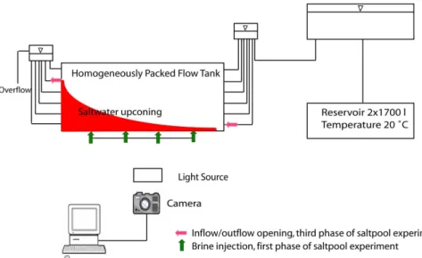
The flow experiments were conducted in a Plexiglas tank with dimensions (L×H×W) of 1.58 m×0.6 ˙m×0.04 m, (Fig. 1 and Fig. 2). The back of the tank holds devices to place the measurement instruments, like the pressure sensors, the electrodes and the
10
temperature sensors. The front side of the tank consists of a clear Plexiglas pane facilitating visual observation of the tracer movement through the homogenous porous medium during the course of the experiments. The tank has four openings at the bottom, which are regulated by valves. Further six openings are placed at the left-hand and right-left-hand side of the tank, respectively. These openings are also regulated
15
by valves and are connected to water reservoirs. The height of the reservoirs can be adjusted to adapt the velocity of the water inside the porous media. Two 1700 l fresh water reservoirs, where the water temperature is kept constant at 20◦C to avoid degassing in the porous media, maintain water supply to the inflow reservoir. Since the Plexiglas walls of the tank slightly deform when the tank is filled with porous media,
20
tension pins with a diameter of 0.5 cm were installed within the tank to prevent the deformation of the tank. Because these obstacles are small, we assume that they do not perturb the flow. Further, a metal bar is placed around the tank to stabilize the tank’s walls. Artificial glass beads with a diameter of 0.5 mm are used as porous media. The tank was homogenously packed. During filling, there was always more water in
25
the tank than glass beads in order avoid air trapping. A neoprene sheet and air tubes were placed between the Plexiglas cover and the porous media. The air tubes can be inflated to compensate for the free space when the glass beads compact, preventing
HESSD
4, 4175–4210, 2007 Concentration determination on flow tank experiments M. Konz et al. Title Page Abstract Introduction Conclusions References Tables Figures ◭ ◮ ◭ ◮ Back CloseFull Screen / Esc
Printer-friendly Version Interactive Discussion
EGU
thus preferential flow along the top cover of the tank. A supplementary experiment with traced water and horizontal flow conditions revealed that there are no preferential pathways and that the water flows homogenously through the porous media.
The experiments E2 and E3 in Table 1 (Sect. 3.5) consisted of four phases. The brine with an initial concentration of 100 g/l was marked with 1 g/l of the red food dye
5
Cochineal Red A (E124). In the first phase of the experiment the brine was pumped into the domain from four openings at the bottom of the tank, as indicated in Fig. 1 by the green arrows. Buoyancy effects forced the brine to move laterally in the second phase and form a planar brine-freshwater interface. No flow was applied in this second phase through any openings of the tank. At the end of this phase, the brine had equilibrated
10
with a mixing zone of about 4 cm above 3 cm of brine with the initial concentration of 100 g/l. The head difference between inflow and outflow reservoirs generated a constant flow during the third phase of the experiment, which we refer to as the flow phase in the following. Flow through the inflow opening on the lower left-hand side of the tank (11 cm above the ground, red arrow in Fig. 1), close to the brine and the
15
outflow opening on the upper right-hand side of the tank (45 cm above the ground, red arrow in Fig. 1) forced an upconing of the saltwater below the outlet as shown in Fig. 1 by the red line. Mechanical dispersion and advection processes cause the upconing of the saltwater. The last phase is the calibration phase to enable the conversion of dye intensities to concentrations, details on this phase can be found in Sect. 3.4.
20
3 Concentration determination with photometry
3.1 Image acquisition and general concept of optical concentration determination The dense fluid was marked with a dye to visually differentiate the salt water from the ambient pore water. Cochineal Red A (E124) was used as tracer. This food dye is nonsorbing, relatively inert, and mostly nonreactive with NaCl in concentrations used
25
HESSD
4, 4175–4210, 2007 Concentration determination on flow tank experiments M. Konz et al. Title Page Abstract Introduction Conclusions References Tables Figures ◭ ◮ ◭ ◮ Back CloseFull Screen / Esc
Printer-friendly Version Interactive Discussion
EGU
analysis of different dye-saltwater solutions revealed that there is no degradation or op-tical decay of dye over a period several days. To determine concentration distributions in the tank we took photos with a digital camera (Nikon D70) using a reproducible illu-mination with a single light source placed right above the camera in a distance of ∼3 m from the tank. The light source (EKON JM-T 1x400 W, E40) was adjusted and checked
5
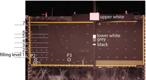
with a luxmeter to minimize spatial lightning nonuniformity. However, it was not possi-ble to totally avoid lightning nonuniformity and a higher intensity remains in the centre of the photographed domain. White, grey and black cards are attached on the front pane of the tank (Fig. 2). A dark curtain placed around the entire experimental setup prevented reflections of any objects on the tank pane. Furthermore, there were no
10
windows in the laboratory in order to avoid lightning nonuniformity due to daylight. All camera parameters were set manually (1/8s, f/13, ISO200). For image processing it is important that images, taken at different times, match on a pixel by pixel basis. There-fore, a computer programme (Nikon camera controlPRO) controlled the camera which was not touched or removed during the entire experiment including the calibration
pro-15
cedure. The digital camera stores raw data (.nef) beside the automatically non-linearly processed photos (.jpg). The raw data are linear measurements of reflected intensities. The image-processing procedure includes the following steps: (1) data converting to 16 bit tif images (65 536 intensity values per channel of the RGB color space) with the freeware dcraw (http://cybercom.net/∼dcoffin/dcraw/), (2) selection of green channel
20
(most sensitive to dye concentrations), (3) correction of fluctuations in brightness, (4) determination of measurement area, (5) construction of a curve that relates intensities to concentrations from calibration images and determination of function parameters for the mathematical formulation of the curve, and (6) conversion of measured intensities of the experiment into concentrations. In the following, steps 3 to 6 are described in
25
HESSD
4, 4175–4210, 2007 Concentration determination on flow tank experiments M. Konz et al. Title Page Abstract Introduction Conclusions References Tables Figures ◭ ◮ ◭ ◮ Back CloseFull Screen / Esc
Printer-friendly Version Interactive Discussion
EGU
3.2 Correction of fluctuations in brightness (step 3)
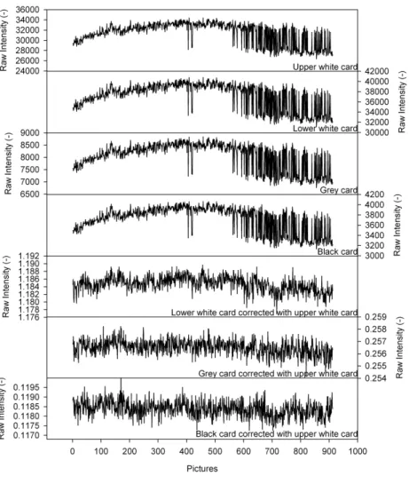
A constant light source is difficult to realize because of fluctuations in energy supply. The first four graphs in Fig. 3 show the intensities of attached white, grey and black cards (see Fig. 2 for the position of the cards), which are strongly influenced by the fluctuations in lightning. These fluctuations were corrected, Icorr,i ,j, with the attached
5
upper white card. The intensities of the images (Ii ,j) were divided by the intensity of the white card (Iwhite) of the respective image. The last three graphs in Fig. 3 show how
the correction method is applied for the lower white card, the grey and black cards. As a consequence, the images are on the same intensity level after the correction step and changes in intensity do only result from changes in dye concentration and not
10
from fluctuation in lightning. Minor fluctuations still persist and are related to scattered reflection on the camera lens, which cannot be corrected. These uncertainties are treated in the error estimation in Sect. 3.5.
3.3 Impact of optical heterogeneity of porous media and determination of measure-ment area (step 4)
15
The resolution of the images is crucial especially in experiments where concentra-tions spatially vary with a steep gradient, e.g. in transition zones. In the literature, little attention has been paid to analyze the impact of the resolution on the precision of the derived concentration data. Schincariol et al. (1993) suggested a general median smoothing (3×3 pixels) to reduce noise from bead size. The image resolution of our
20
digital images (approx. 0.31 mm2/pixel) implies a high resolution of the punctual con-centration determination. In order to analyze the impact of resolution, we took images of all calibration steps (0–100 g/l) and analyzed the intensity distributions in squares of 25 cm2(8100 pixels) at different positions of the image. The squares were equally filled with the respective solution and due to the small extent of 25 cm2the impact of uneven
25
lightning can be excluded. Figure 4a shows exemplarily the intensities of one of the squares for 100 g/l derived from 1×1 pixel and from the median over 5×5, 10×10 and
HESSD
4, 4175–4210, 2007 Concentration determination on flow tank experiments M. Konz et al. Title Page Abstract Introduction Conclusions References Tables Figures ◭ ◮ ◭ ◮ Back CloseFull Screen / Esc
Printer-friendly Version Interactive Discussion
EGU
18×18 pixels. The fluctuation of intensities increases with increasing resolution due to the noise from bead size or the position of the beads.
The comparison of the 95% confidential intervals in Fig. 4b shows that the precision of the averaged values increases with increasing edge length. These patterns apply to all concentrations and are exemplarily demonstrated for 100 g/l. The calculated
inten-5
sities significantly vary for resolutions smaller than 102pixels. In this study an average over 100 pixels (10 pixels edge length) is taken to calculate punctual concentrations. This corresponds to an area of about 31 mm2. The actual resolution for concentration determination is therefore lower than the image resolution itself.
3.4 Image calibration and converting of intensities to concentrations (step 5 and 6)
10
Existing methods of image processing convert measured intensities into optical den-sities based on intensity vs. optical density standard curve. The reference values of optical density are taken from an attached grey scale. This step is necessary if ana-logue photography is used and the photos have to be developed and scanned. Differ-ences in lightning, exposure, film development and scanning of the images can cause
15
fluctuations in the raw data, which are corrected using the intensity vs. optical density standard curve. Each image has to be processed this way which requires large CPU time if the number of images is large. The relation between optical density and con-centrations is determined by separate calibration experiments where the tank is filled with different solutions (Schincariol et al., 1993).
20
This procedure is very CPU consuming if time series of concentrations should be calculated, the parameters of the intensity-optical density standard curves have to be derived by optimization for each image. Since we do apply digital photography, errors caused by scanning or film development are excluded and the computation of the op-tical densities for each image is not necessary. The brightness-corrected images (see
25
Sect. 3.2) can directly be translated to concentrations based on intensity vs. concen-tration standard curves, which have to be derived for each point where concenconcen-trations should be determined.
HESSD
4, 4175–4210, 2007 Concentration determination on flow tank experiments M. Konz et al. Title Page Abstract Introduction Conclusions References Tables Figures ◭ ◮ ◭ ◮ Back CloseFull Screen / Esc
Printer-friendly Version Interactive Discussion
EGU
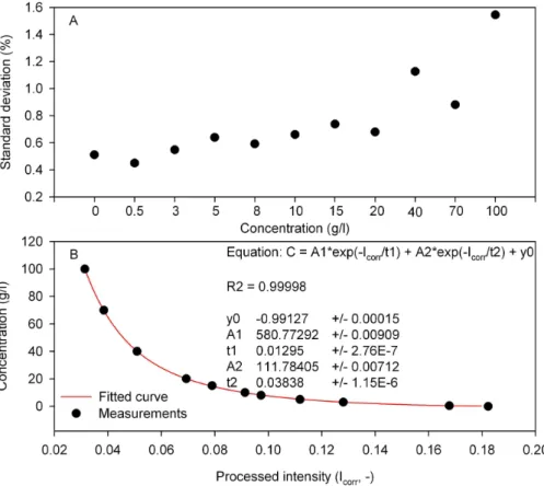
In our experiment not the tracer concentration itself is of interest but the salt concen-tration. Therefore, we directly relate intensities of the dye to salt concentrations. In the calibration experiment, also referred to as calibration phase of the experiment, solu-tions of predetermined salt water-dye concentrasolu-tions (0.5, 3, 5, 8, 10, 15, 20, 40, 70, 100 g/l of salt water, the dye concentration is always 1/100 of the salt concentration)
5
were pumped in the tank from the bottom of the tank upwards in a sequential order from low-density solutions to high-density solutions. This prevents instabilities and en-ables a uniform filling of the domain. 50 images were taken from each calibration step. The average intensity value of each calibration step is then used to derive the specific calibration curves (Fig. 5b).
10
The theoretical relation between intensity and concentration (in case of transmit-tance) follows an exponential function. This relation is known as Lambert-Beer’s law and it is valid for monochromatic light and for solutions without porous media. Because this is not the case in our experiments, we tried various functions to relate intensity and concentration (power laws of higher order and exponential functions). A second
15
order exponential function turned out to be the most suitable to relate intensities to concentrations (see Fig. 5b).
The parameters of the calibration curve had to be derived for each specific obser-vation point. Thus, background levelling, as suggested in Schincariol et al. (1993) to account for spatially uneven lightning of the tank, was not necessary. Once the
param-20
eters of the standard curve are determined they apply to all experiments if illumination and camera position is constant. This approach offers a computational effective way to derive high-resolution time series of concentrations.
3.5 Impact of lens flare on measured intensities
The basis of photometry in terms of concentration measurements of fluids is the
fol-25
lowing: the brightness of two solutions is of equal intensity during calibration and all stages of the experiment, if the solutions are equally concentrated (Arnold et al., 1971). However, this prerequisite might be perturbed due to effects of lens flare. Rogers (in
HESSD
4, 4175–4210, 2007 Concentration determination on flow tank experiments M. Konz et al. Title Page Abstract Introduction Conclusions References Tables Figures ◭ ◮ ◭ ◮ Back CloseFull Screen / Esc
Printer-friendly Version Interactive Discussion
EGU
Newman, 1976) stated: “one of the most usual problems created by white backgrounds is that of flare, caused by excessive reflection from white surface into the camera lens . . . .” In porous media experiments the artificial glass beads cause high reflection in-tensity and might generate flare effects, which have enough inin-tensity to perturb the measurements. Regions of the photographed domain, which have a high dye
con-5
centration, might appear brighter because of the lens flare effects. That causes an underestimation of concentrations. We conducted a series of experiments in order to investigate the impact of lens flare effects on reflected intensity measurements (Ta-ble 1).
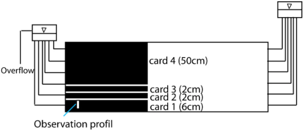
In experiment E1 we successively placed four 70 cm long black cards one after
an-10
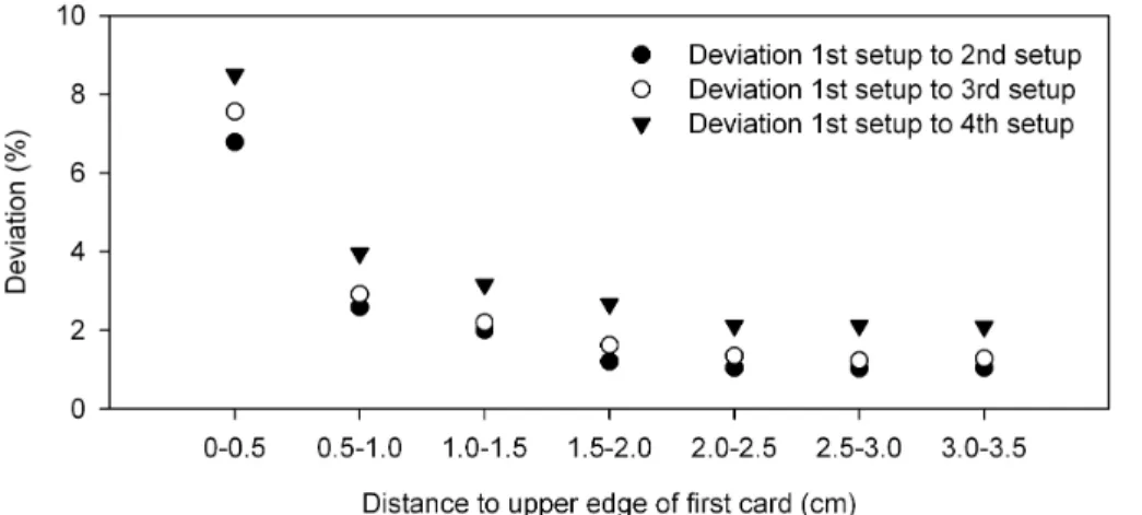
other at the left side of the front window of our tank as illustrated in Fig. 6. 50 images were taken of each of the 4 steps. Figure 7 shows the decline of intensities along a vertical profile on card 1 (Fig. 6) for the four steps of the experiment. Adding cards 2–4 above card 1 decreases the reflection from the porous media above card 1 and therefore the effect of flare was reduced and made card 1 appear darker.
15
The fourth stage of E1 is comparable to the calibration phase of E2 (see Sect. 3.4) when the entire tank was filled with the coloured saltwater and lens flare is widely reduced. However, the dye tracer did not affect the largest portion of the tank during the flow phase of E2 and reflection intensity of the porous media was high. The shape of the salt body during the upconing process of the flow phase of E2 is schematically
20
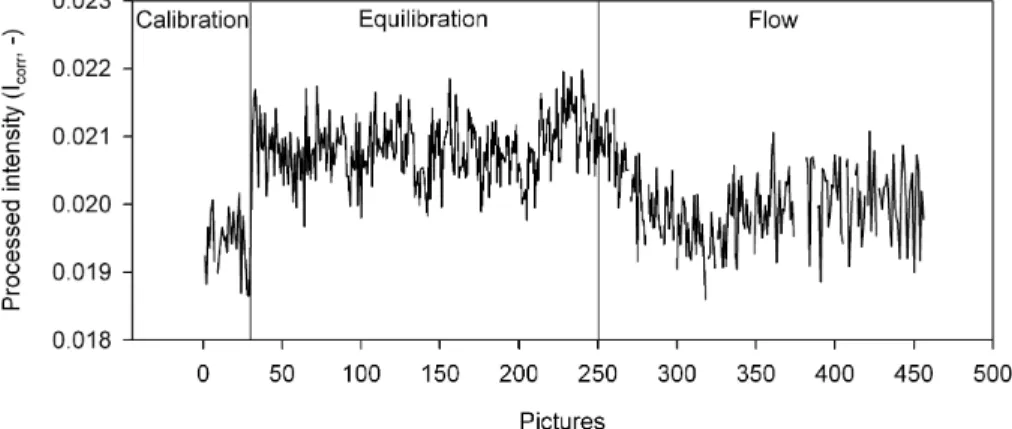
shown in Fig. 1. Flare effects like in E1 can occur. In order to demonstrate the flare effects in E2 we exemplarily derived intensities at a point 2 cm above the ground. The position of this measurement point is equal to the observation hole P1 of E3 (Fig. 2). Concentration profiles showed that the transition zone of the salt water in the end of the equilibration phase, the second phase of the saltpool experiment, started 3 cm above
25
the ground. Therefore, the concentration is necessarily 100 g/l at 2 cm above ground. Since the salt body moves upwards to the outlet during the course of the experiment no concentration changes are expected at this point. The intensities in Fig. 8 show a clear shift from 100 g/l calibration to the equilibration phase (app. 7% increase of intensity)
HESSD
4, 4175–4210, 2007 Concentration determination on flow tank experiments M. Konz et al. Title Page Abstract Introduction Conclusions References Tables Figures ◭ ◮ ◭ ◮ Back CloseFull Screen / Esc
Printer-friendly Version Interactive Discussion
EGU
and from calibration to the flow phase (app. 3%). The intensity values decline during the upconing process of the flow phase. With the upconing of the saltwater the coloured water affects a larger region around the observation point and reflection intensities are reduced. Therefore, the flare effects are reduced and the deviation between calibration intensities for 100 g/l and the measured intensities during the flow phase decline to
5
3%. This effect is comparable to the effects observed in E1 when the black cards are attached above card 1.
Rogers (in Neuman, 1976) suggested: “this problem (of lens flare) is largely over-come (. . . ) and reduced to a minimum by masking the background area so that as little as possible is displayed.” Therefore, we attached a mask on the photographed
do-10
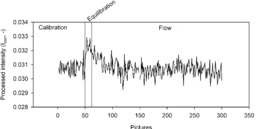
main with holes (1.5×1.5 cm2) at those points where we wanted to derive breakthrough curves for the third experiment E3 (Fig. 2). The upconing took place at the left side of the domain below the outlet. Therefore, as much observation points as possible were distributed in or close to the area of the expected salt water upconing. Figure 9 shows the intensities of P1 during all stages of the experiment. It gets obvious that the effect
15
of lens flare is strongly reduced especially during the flow phase (0% intensity devia-tion between calibradevia-tion and flow phase). However, there is still app. 3% of deviadevia-tion between calibration and the equilibration phase of E3. We refer this effect to the impact of the observation points close to P1. These were not influenced by the dye and there-fore reflection intensity was high and, hence, could cause lens flare effects. During the
20
course of the experiment the salt plume rose and the points in the neighbourhood of P1 appeared darker, which reduced flare effects during the flow phase comparable to the effects observed in E1 and E2. Therefore, the attached mask helps to reduce flare effects.
The experiment E4 was conducted to estimate the error caused by flare effects.
25
Solutions of predetermined 5, 40, and 100 g/l (salt+dye) were progressively pumped into the tank from the bottom upward. Seven different filling levels with a horizontally planar salt water front were realized so that all observation points in the same horizontal line were fully immerged in the solution. In order to estimate the impact of lens flare we
HESSD
4, 4175–4210, 2007 Concentration determination on flow tank experiments M. Konz et al. Title Page Abstract Introduction Conclusions References Tables Figures ◭ ◮ ◭ ◮ Back CloseFull Screen / Esc
Printer-friendly Version Interactive Discussion
EGU
derived intensities at all observation points for all filling levels of the experiment of the three solutions and analyzed their development during the course of the experiment. E4 revealed that the error depends on (i) the concentration of the solution, and the error increases with increasing concentration; on (ii) the intensity of the neighboring observation points, while the error decreases with decreasing intensity.
5
The maximal deviation of intensities for the 100 g/l solution in E4 amounted to 3%. This experiment only shows 1-D vertical movement of the brine, whereas 2-D plume shapes such as in the saltpool experiments E2 and E3 do not occur. Therefore, we do use the results of E4 only to estimate the error caused by lens flare effects and not to correct the measured data. We assume a maximal error of 3% of overestimation
10
(compared to calibration) of the intensities during the flow phase caused by lens flare effects.
In order to estimate the precision of the photometric method we calculated the stan-dard deviation of the calibration images for each calibration step (Fig. 5A). The maximal deviation, which we consider as accuracy of the measured intensities is ±1.5% for salt
15
concentration of calibration step 100 g/l. From the above discussion we know that there is an additional error of +3%. Therefore, the concentrations are given with confidential limits (see Fig. 15). The lower boundary is calculated from the processed intensity Icorr
minus 1.5% of error, whereas for the upper boundary Icorrplus 4.5% is used to derive
concentrations.
20
4 Concentration determination with resistivity measuring cells (RMC)
The resistivity measured between two electrodes is a function of the porous material, porosity, temperature, geometrical arrangement of the electrodes, state of gold coat-ing and the ion concentration. Durcoat-ing an experiment all factors apart from the ion concentration are kept constant and the measured resistivity can be related to the
con-25
centration of the solution surrounding the electrodes. Theory on resistivity methods is well documented, e.g. in Telford et al. 1990. In this paper we will present constructional
HESSD
4, 4175–4210, 2007 Concentration determination on flow tank experiments M. Konz et al. Title Page Abstract Introduction Conclusions References Tables Figures ◭ ◮ ◭ ◮ Back CloseFull Screen / Esc
Printer-friendly Version Interactive Discussion
EGU
details of the measurement and data acquisition system.
Resistivity measurements to determine salt concentrations are widely used and com-mercial systems are available for measurements outside the porous media flow tank. However, standard commercial electrode systems are not applicable for in situ mea-surements in porous media experiments. An adequate measurement system for in situ
5
measurement of conductivity in porous media has to cover a wide concentration range (0–300 g/l salt concentration) and the perturbation of the flow field must be minimal. In cooperation with Edi Meier and Partner AG we developed a new resistivity measure-ment system to determine salt concentrations over a concentration range from 0 to 300 g/l within the porous media.
10
4.1 Technical setup of the RMC system
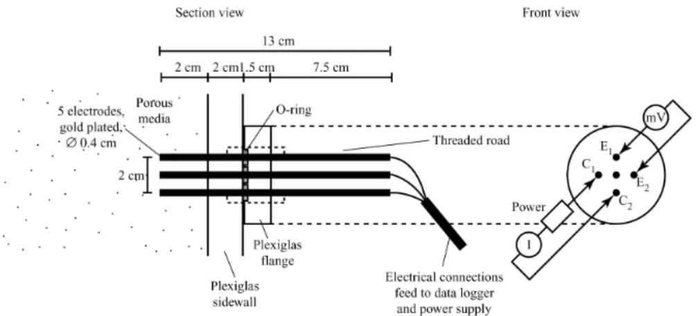
Each RMC consists of five gilded stainless steel electrodes (ø 0.4 cm, length 13 cm, Fig. 10). We need gilded electrodes, because uncontrollable fluctuations in the resis-tivity measurement occur with ungilded stainless steel electrodes. The electrodes are equally spaced 1 cm around the center electrode and mounted on a Plexiglas flange.
15
They are installed perpendicular to the flow direction through the back wall of the tank. Figure 11 shows the schematic construction plan of the entire RMC system. The sys-tem involves measuring the output voltage between the electrodes E1 and E2 while electrical current is caused to flow through the porous media between the outer pair of electrodes C1 and C2. The grounding electrode is in the center. The measuring
20
principle bases on a 4-electrode resitivity measurement technique, where the current is supplied through a very precisely regulated sinusoidal oscillator signal. The mea-sured AC-voltage is rectified through a synchronous demodulator in phase to the os-cillator. The resulting DC output voltage was recorded utilizing a micro-logger and a relais based multiplexer to measure all the RMCs sequentially. An alternating current
25
was applied in all measurements to minimize polarization within the cell and to prevent movement of the ions due to the presence of a voltage potential.
HESSD
4, 4175–4210, 2007 Concentration determination on flow tank experiments M. Konz et al. Title Page Abstract Introduction Conclusions References Tables Figures ◭ ◮ ◭ ◮ Back CloseFull Screen / Esc
Printer-friendly Version Interactive Discussion
EGU
salt concentrations two different input voltages are used at each time step. This en-ables the measurement in two measurement ranges, one for the high concentration, referred to as MR1, and the other one for the low concentrations, MR2. As this mea-suring method is sensitive to temperature variations, temperature sensors (YSI 4006; accuracy ±0.01◦C) are also implemented into the same porous medium.
5
4.2 Electrode arrays
Various electrode arrays were tested in preliminary experiments in a small container (35×16×9 cm3) filled with saturated porous media. Figure 12 shows the three investi-gated arrays. In array 1 all electrodes are uniformly placed in a line with the grounding electrode in the center. Array 2 is a cross-placement of C1,2 (current electrodes) and
10
E1,2 (potential electrodes) while in array 3 input and output electrodes are placed in a
neighbouring position (parallel). In preliminary tests to evaluate the best array setup the three different arrays were also rotated clockwise to study the influence of the flow di-rection of the saltwater front. Array 1 was rotated clockwise by 90◦, array 3 was rotated clockwise by 90◦, 135◦, 180◦ and 315◦. A total of 4 tests were carried out. The setups
15
were evaluated by measuring a successively rising saltwater front in the small experi-mental tank. Figure 13 shows the measured breakthrough curves of output voltages of the 8 different arrangements.
The breakthrough curves of array 1 and its clockwise rotated (by 90◦) setup clearly show the dependence of these alignments to the flow direction of the salt front. There is
20
a temporal shift between both curves and array 1 even shows a horizontal course of the curve. Array 2 delivers no analyzable breakthrough curve. In this setup both electrodes should detect the same voltage under homogeneous conditions. The fact that a voltage change is visible might be due to local concentration differences or unsymmetrical manufacturing of the RMC. Array 3 and its rotated setups deliver curves less dependent
25
on the flow direction of the front and a realistic shape of the curve is observed. Due to these results we chose array 3 to align the electrodes.
HESSD
4, 4175–4210, 2007 Concentration determination on flow tank experiments M. Konz et al. Title Page Abstract Introduction Conclusions References Tables Figures ◭ ◮ ◭ ◮ Back CloseFull Screen / Esc
Printer-friendly Version Interactive Discussion
EGU
4.3 Calibration of the RMC
The output voltage as a function of the porous media type, porosity, temperature, ge-ometrical arrangement of the electrodes, state of gold coating and the concentration of the surrounding solution is measured between electrodes E1and E2. Since all
fac-tors affecting the measurement are kept constant the output voltage can directly be
5
related to the ion concentration of the solution. This relationship has to be determined via calibration experiments as described in Sect. 3.4. The output voltages of the two measuring ranges, MR1 and 2, are correlated with the concentrations using specifically fitted power laws for each RMC and measurement range. Figure 14 shows exemplar-ily the calibration curves for MR1 and 2 of the RMC located at observation point P2
10
(Fig. 2).
The errors associated with the concentration consist of two parts: measurement errors and errors associated with the calibration curves. The measurement errors are small and the maximum error found during the calibration experiment was ±0.5%. The errors associated with the calibration curve are within the range −1.5 to +2.5%. Since
15
the calculated error is small we do not show error bars in Fig. 15. Typically, systematic errors are caused by temperature fluctuations. However, these can be minimized for laboratory experiments due to controlled room and water temperature.
5 Comparison of both methods
For direct comparison of the RMC method and the image analysis method we derived
20
concentrations from the images at the position of the centre electrode of the RMC at observation points P2 and P3 (Fig. 2). The comparison reveals that both independent methods reproduce the expected concentrations of 100 g/l at P2 when the salt wa-ter rises, although the RMC shows a slightly earlier reaction than the image analysis approach, what can be explained with the larger measurement volume (Fig. 15).
25
concen-HESSD
4, 4175–4210, 2007 Concentration determination on flow tank experiments M. Konz et al. Title Page Abstract Introduction Conclusions References Tables Figures ◭ ◮ ◭ ◮ Back CloseFull Screen / Esc
Printer-friendly Version Interactive Discussion
EGU
tration gradients exist, the two methods differ significantly due to the different mea-surement volumes, as it is the case at P3 (Fig. 15). The RMC measures an apparent resitivity of the environment around the electrodes. Thus, it is not a point-wise mea-surement but an integral value. The meamea-surement volume strongly depends on the ion concentration distribution and on the resistivity contrast during the experiment.
There-5
fore, the measurement volume is not constant throughout the course of the experiment. This problem is the major drawback of the RMC method especially for measuring points within the transition zone, where a concentration gradient occurs within the mea-suring volume of the RMC. However, especially for points where the electrodes are surrounded by a uniform concentration, like P2 this problem is of minor importance. A
10
numerical simulation of the resistivity field, the current density and of the voltage at the electrodes for heterogeneous resistivity distributions could enable the determination of the measurment volume. This work was beyond the scope of this study but we highly recommend further investigation in this field.
6 Conclusions
15
In this study we present a photometric methodology, which enables effective computa-tion of high-resolucomputa-tion time series of plume concentracomputa-tions. The approach is capable to treat a large number of images since only one optimization of the intensity vs. concen-tration standard curve is required. Once the parameters of this curve are known for the observation point they can be used for a series of experiments, if the camera position
20
and the tank position do not change and the images fit on a pixel by pixel basis. The resolution of the observation point is crucial for the precision of the measured inten-sity values. Therefore, we suggest a statistical analysis for each experimental setup to determine the adequate resolution.
A major source of error is the impact of lens flare. High reflections of bright regions
25
of the photographed domain, which are not influenced by the dye, could generate flare effects that increase the measured intensity of dark, dye-influenced regions of the tank.
HESSD
4, 4175–4210, 2007 Concentration determination on flow tank experiments M. Konz et al. Title Page Abstract Introduction Conclusions References Tables Figures ◭ ◮ ◭ ◮ Back CloseFull Screen / Esc
Printer-friendly Version Interactive Discussion
EGU
This leads to an underestimation of the concentration. Attaching a mask at the front window of the tank, which reduces the percentage of bright regions, can minimize this effect. However, only information at the predetermined points, i.e. the observation holes in the mask, is available in this case. Since the mask itself influences the brightness of the observation holes, both the calibration and the flow experiments have to be
5
conducted using the same setup with the mask. This minimizes the flexibility of the experiment in order to run different experiments with changing boundary conditions and therefore with different plume patterns.
Nevertheless, the precision of the measurement is high even without the mask. A successive filling of the tank with predetermined concentrations of salt-dye solutions
10
enables an estimation of the error caused by flare effects. The successive filling grad-ually reduced the percentage of bright regions and therefore decreased the impact of flare effects at the observation points. The deviation between the measured intensity of the entirely filled tank and the partly filled tank was determined as maximal error. A more detailed error determination is, to our experience, difficult to realize.
15
The newly developed resitivity measurement system provides highly precise mea-surements of output voltages, which can be translated into concentrations using a fit-ted power law. The major perturbations of the measurement are temperature changes, which can be avoided in laboratory scale experiments. However, the main drawback of the resistivity method is the unknown measurement volume. For the comparison with
20
numerical codes it is crucial to know the exact volume especially in an intermediate scale experiment where even over a few centimetres significant variations in concen-trations occur. Therefore, we consider the image analysis approach as more suitable to derive breakthrough curves for benchmarking numerical codes. The electrodes, how-ever, can be used to cross-check the results of the image analysis method at points of
25
uniform concentration distribution.
For future research we suggest transmissive measurements of intensity. This was not possible in our case due to the measurement systems placed on the back wall of the tank. The glass beads act as prism and therefore a spatially more homogenous
HESSD
4, 4175–4210, 2007 Concentration determination on flow tank experiments M. Konz et al. Title Page Abstract Introduction Conclusions References Tables Figures ◭ ◮ ◭ ◮ Back CloseFull Screen / Esc
Printer-friendly Version Interactive Discussion
EGU
lightning could be realized. The transmissive intensity of the clear porous media without dye is much lower than the reflected intensity what automatically should reduce flare effects. A numerical analysis of the measurement volume of the RMC system could help to improve the applicability of the technique for detailed laboratory-scale flow ex-periments. Regarding hydrogeological field observations, the RMC method could be
5
further developed for multi-level monitoring of electrical conductivities in the context of highly saline groundwaters mixing up with groundwaters of low salinity. This is of spe-cial interest in active evaporite subrosion and/or forced groundwater circulation sys-tems (active pumping).
Acknowledgements. The authors are thankful to C. Veith (IMFS, Strasbourg) who did the
con-10
structional work of the Plexiglas flow tank and to Prof. Wieland for support during the develop-ment of the RMC method. This study was financed by the Schweizer Nationalfond 200020– 109200.
References
Arnold, C., Rolls, P., and Stewart, J.: Applied photography, The Focal Press, ISBN
0-240-15
50723-1, 1971.
Barth, G. R., Illangesekare, T. H., Hill, M. C., and Rajaram, H.: A new tracer-density criterion for heterogeneous porous media, Water Resour. Res., 37, 21–31, 2001.
Diersch H. J. and Kolditz, O: Variable-density flow and transport in porous media: approaches and challenges, Adv. Water Res., 25, 899–944, 2002.
20
Goswami, R. and Clement, P.: Laboratory-scale investigation of saltwater intrusion dynamics, Water Resour. Res., 43, W04418, doi:10.1029/2006WR005151, 2007.
Hassanizadeh, S. M. and Leijnse, A.: A non-linear theory of high-concentration-gradient dis-persion in porous media, Adv. Water Resour., 18, 4, 203–215, 1995.
McNeil, J. D., Oldenborger, G. A., and Schincariol, R. A.: Quantitative imaging of contaminant
25
distributions in heterogeneous porous media laboratory experiments, J. Contam. Hydrol., 84 , 36–54, 2006.
Oostrom, M., Dane, J. H., Guven, O., and Hayworth, J. S.: Experimental investigation of dense solute plumes in an unconfined aquifer model, Water Resour. Res., 28, 2315–2326, 1992.
HESSD
4, 4175–4210, 2007 Concentration determination on flow tank experiments M. Konz et al. Title Page Abstract Introduction Conclusions References Tables Figures ◭ ◮ ◭ ◮ Back CloseFull Screen / Esc
Printer-friendly Version Interactive Discussion
EGU
Oostrom, M., Hofstee, C., Lenhard, R. J., and Wietsma, T. W.: Flow behavior and residual sat-uration formation of liquid carbon tetrachloride in unsaturated heterogeneous porous media, J. Contam. Hydrol., 64, 93–112, 2003.
Oswald, S., Kinzelbach, W., Greiner, A., and Brix, G.: Observation of flow and transport pro-cesses in artificial porous media via magnetic resonance imaging in three dimensions,
Geo-5
derma, 80, 417–429, 1997.
Oswald, S. and Kinzelbach, W.: Three-dimensional physical benchmark experiments to test variable-density flow models, J. Hydrol., 290, 22–42, 2004.
Rahman, A., Jose, S., Nowak, W., and Cirpka, O.: Experiments on vertical transverse mixing in a large-scale heterogeneous model aquifer, J. Contam. Hydrol., 80, 130–148, 2005.
10
Rogers, G.: Photography in paediatrics, Published in photographic techniques in scientific re-search, Volume 2, edited by: Newman, A., Academic Press, ISBN 0-12-517960, 1976. Schincariol, R. A., Herderick, E. E., and Schwartz, F. W.: On the application of image analysis
to determine concentration distributions in laboratory experiments, J. Contam. Hydrol., 12, 197–215, 1993.
15
Silliman, S. E. and Simpson, E. S.: Laboratory evidence of the scale effects in dispersion of solutes in porous media, Water Resour. Res., 23, 1667–1673, 1987.
Silliman, S. E., Zheng, L., and Conwell, P.: The use of laboratory experiments for the study of conservative solute transport in heterogeneous porous media, Hydrogeol. J., 6, 166–177, 1998.
20
Simmons, C. T., Pierini, M. L., and Hutson, J. L.: Laboratory investigation of variable-density flow and solute transport in unsaturated–saturated porous media, Transport Porous Med., 47, 15–244, 2002.
Swartz, C. H. and Schwartz, F. W.: An experimental study of mixing and instability development in variable-density systems, J. Contam. Hydrol., 34, 169–189, 1998.
25
Telford, W. M., Geldart, L. P., and Sheriff, R. E.: Applied geophysics – 2nd edition, Cambridge University Press, ISBN 0-521-33938-3, 1990.
Wildenschild, D. and Jensen, K. H.: Laboratory investigations of effective flow behavior in un-saturated heterogeneous sands, Water Resour. Res., 35, 17–27, 1999.
HESSD
4, 4175–4210, 2007 Concentration determination on flow tank experiments M. Konz et al. Title Page Abstract Introduction Conclusions References Tables Figures ◭ ◮ ◭ ◮ Back CloseFull Screen / Esc
Printer-friendly Version Interactive Discussion
EGU
Table 1. Experiments conducted to analyze the impact of lens flare effects on measured re-flection intensities.
Experiment Number Objective
Successively attached black cards E1 Demonstrate lens flare effects Saltpool flow experiment, as described in E2 Demonstrate the impact of lens flare
Sect. 2; without mask on measured reflection intensities
Saltpool flow experiment, as described in E3 Test a possibility to reduce
Sect. 2; with mask the measurement error
Progressively filling of salt-dye solutions; E4 Estimate the error caused by
HESSD
4, 4175–4210, 2007 Concentration determination on flow tank experiments M. Konz et al. Title Page Abstract Introduction Conclusions References Tables Figures ◭ ◮ ◭ ◮ Back CloseFull Screen / Esc
Printer-friendly Version Interactive Discussion
EGU
Figure 1: Schematic experimental setup.
HESSD
4, 4175–4210, 2007 Concentration determination on flow tank experiments M. Konz et al. Title Page Abstract Introduction Conclusions References Tables Figures ◭ ◮ ◭ ◮ Back CloseFull Screen / Esc
Printer-friendly Version Interactive Discussion
EGU
Figure 2: Tank of E3 with mask to reduce effects of flare and filling levels of E4.
HESSD
4, 4175–4210, 2007 Concentration determination on flow tank experiments M. Konz et al. Title Page Abstract Introduction Conclusions References Tables Figures ◭ ◮ ◭ ◮ Back CloseFull Screen / Esc
Printer-friendly Version Interactive Discussion
EGU
Figure 3: Measured and processed intensity values of grey and black cards.
HESSD
4, 4175–4210, 2007 Concentration determination on flow tank experiments M. Konz et al. Title Page Abstract Introduction Conclusions References Tables Figures ◭ ◮ ◭ ◮ Back CloseFull Screen / Esc
Printer-friendly Version Interactive Discussion
EGU
Figure 4: A: Intensities of the 8281 pixels of a square of 5 cm2 of calibration image 100 g/l Fig. 4. A: Intensities of the 8281 pixels of a square of 5 cm2 of calibration image 100 g/l de-rived as median of squares of 1, 5 and 10 pixels edge length; B: Median of squares of 1×1 to 18×18 pixels and 95% confidential interval.
HESSD
4, 4175–4210, 2007 Concentration determination on flow tank experiments M. Konz et al. Title Page Abstract Introduction Conclusions References Tables Figures ◭ ◮ ◭ ◮ Back CloseFull Screen / Esc
Printer-friendly Version Interactive Discussion
EGU
Figure 5: A: Standard deviation of calibration images at observation point P2 (Figure 2); B Fig. 5. A: Standard deviation of calibration images at observation point P2 (Fig. 2); B: Intensity vs. concentration and fitted second order exponential function for P2.
HESSD
4, 4175–4210, 2007 Concentration determination on flow tank experiments M. Konz et al. Title Page Abstract Introduction Conclusions References Tables Figures ◭ ◮ ◭ ◮ Back CloseFull Screen / Esc
Printer-friendly Version Interactive Discussion
EGU Figure 6: Setup of the experiment E1. The cards are placed one after another righ
Fig. 6. Setup of the experiment E1. The cards are placed one after another right above each other, the heights of the cards are written in brackets.
HESSD
4, 4175–4210, 2007 Concentration determination on flow tank experiments M. Konz et al. Title Page Abstract Introduction Conclusions References Tables Figures ◭ ◮ ◭ ◮ Back CloseFull Screen / Esc
Printer-friendly Version Interactive Discussion
EGU
Figure 7: Deviation (decline) of intensities taken at the profile in Figure 6 when adding cards
Fig. 7. Deviation (decline) of intensities taken at the profile in Fig. 6 when adding cards above card 1.
HESSD
4, 4175–4210, 2007 Concentration determination on flow tank experiments M. Konz et al. Title Page Abstract Introduction Conclusions References Tables Figures ◭ ◮ ◭ ◮ Back CloseFull Screen / Esc
Printer-friendly Version Interactive Discussion
EGU
Figure 8: Intensities of P1 (however without mask) where no concentration changes occur Fig. 8. Intensities of P1 (however without mask) where no concentration changes occur during the flow phase of the density flow experiment (constant concentration of 100 g/l).
HESSD
4, 4175–4210, 2007 Concentration determination on flow tank experiments M. Konz et al. Title Page Abstract Introduction Conclusions References Tables Figures ◭ ◮ ◭ ◮ Back CloseFull Screen / Esc
Printer-friendly Version Interactive Discussion
EGU
Figure 9: Intensities of observation point P1 with mask. Fig. 9. Intensities of observation point P1 with mask.
HESSD
4, 4175–4210, 2007 Concentration determination on flow tank experiments M. Konz et al. Title Page Abstract Introduction Conclusions References Tables Figures ◭ ◮ ◭ ◮ Back CloseFull Screen / Esc
Printer-friendly Version Interactive Discussion
EGU
Figure 10: Electrode array with two current electrodes (C and C ), two potential electrodes Fig. 10. Electrode array with two current electrodes (C1and C2), two potential electrodes (E1and E2) and grounding in the center of the array.
HESSD
4, 4175–4210, 2007 Concentration determination on flow tank experiments M. Konz et al. Title Page Abstract Introduction Conclusions References Tables Figures ◭ ◮ ◭ ◮ Back CloseFull Screen / Esc
Printer-friendly Version Interactive Discussion EGU C1 C2 E1 E2 + - = ~ ~ D A 2500 mV FS 250 mV FS Logger
Amplifier Rectifier AD Converter
Oscillator 21 V p-p 3.4 kHz 1µ F 1µ F High conductivity range HC Low conductivity range LC 6.8 kW 680 W RMC Switch
HESSD
4, 4175–4210, 2007 Concentration determination on flow tank experiments M. Konz et al. Title Page Abstract Introduction Conclusions References Tables Figures ◭ ◮ ◭ ◮ Back CloseFull Screen / Esc
Printer-friendly Version Interactive Discussion
EGU
Figure 12: Evaluated sets of electrode arrays.
Fig. 12. Evaluated sets of electrode arrays.HESSD
4, 4175–4210, 2007 Concentration determination on flow tank experiments M. Konz et al. Title Page Abstract Introduction Conclusions References Tables Figures ◭ ◮ ◭ ◮ Back CloseFull Screen / Esc
Printer-friendly Version Interactive Discussion
EGU
Fig. 13. Measured breakthrough curves of output voltage (mV) for the different sets of elec-trodes and their clockwise-rotated arrangements.
HESSD
4, 4175–4210, 2007 Concentration determination on flow tank experiments M. Konz et al. Title Page Abstract Introduction Conclusions References Tables Figures ◭ ◮ ◭ ◮ Back CloseFull Screen / Esc
Printer-friendly Version Interactive Discussion
EGU
Figure 14: Calibration curves for the RMC at P2. Fig. 14. Calibration curves for the RMC at P2.
HESSD
4, 4175–4210, 2007 Concentration determination on flow tank experiments M. Konz et al. Title Page Abstract Introduction Conclusions References Tables Figures ◭ ◮ ◭ ◮ Back CloseFull Screen / Esc
Printer-friendly Version Interactive Discussion
EGU
Fig. 15. Breakthrough curves of P2 (100 g/l) and P3 (max. 30 g/l) derived from electrodes and from photometric method. The solid lines represent the range of error of the photometric method.