A 2-d dynamical model of mesospheric temperature inversions in winter

HAL Id: insu-03130834

https://hal-insu.archives-ouvertes.fr/insu-03130834

Submitted on 4 Feb 2021

HAL is a multi-disciplinary open access

archive for the deposit and dissemination of

sci-entific research documents, whether they are

pub-lished or not. The documents may come from

teaching and research institutions in France or

abroad, or from public or private research centers.

L’archive ouverte pluridisciplinaire HAL, est

destinée au dépôt et à la diffusion de documents

scientifiques de niveau recherche, publiés ou non,

émanant des établissements d’enseignement et de

recherche français ou étrangers, des laboratoires

publics ou privés.

A 2-d dynamical model of mesospheric temperature

inversions in winter

Alain Hauchecorne, Alexandre Maillard

To cite this version:

Alain Hauchecorne, Alexandre Maillard. A 2-d dynamical model of mesospheric temperature

inver-sions in winter. Geophysical Research Letters, American Geophysical Union, 1990, 17 (12),

pp.2197-2200. �10.1029/GL017i012p02197�. �insu-03130834�

GEOPttYSICAL RESEARCtt I,ETI'ER$, VOL,. I7, NO. !2, PAGES 2197-2200, NOVEMBER 1990

A 2-D DYNAMIC• MODEL OF MESOSPHERIC TEMPERATURE INVERSIONS IN WINTER

Alain Hauchecorne and Alexandre Maillard

Service d'Atronomie du CNRS, Verri•res-le Buisson, France

Abstract: A 2-D stratospheric and mesospheric dynami-

ca/model including drag and diffusion due to gravity wave

breaking is used to simulate winter mesospheric temperature

inversions similar to those observed by Rayleigh !idar. It is shown that adiabatic heating associated to descending veloci- ties 'm the mesosphere is the main mechanism involved in the

formation of such inversions. Sensitivity tests are performed Mth the model and confirm this assumption. It is also ex-

phined why other previous similar studies with 2-D models did not show mesospheric inversion layers.

Introduction

A strong inversion layer is very often observed in me-

sospheric temperature profiles with a relative minimum of temperature around 70 km, and a positive temperature gradi- ent in the few kilometers above this minimum. This feature has been first observed by rocket meas•ements and reported by Schmidlin [1976] but without explanation of the phe-

nomenon. More recently local deficiencies of the density, as- sociated with temperature inversion layers, were observed from the reentry data of the US space shuttle [Champion, 1986!. The first statistical study of these inversion layers has been made •Sth a large data base of more than 1000 tempera- ture profiles obtained by two Rayleigh lidars located in the south of France [Hauchecorne et al., 1987, hereafter HCW]. This study showed that the probability of occurrence of an in- version presents a maximum of 70 % in winter. These inver-

sions are observed at the same altitude during several days

and usually simultaneously above the two lidar sites (disrace

between the two sites: 550 km). The similarity between the characteristics of the inversions and of the MST radar echoes in the mesosphere, leads HCW to conclude that both phenom- ena have the same origin, that is to say the breaking of up- ward propagating internal gravity waves. Using a crude es-

timate of the amplitude growth with height of a gravity wave,

HCW showed that gravity waves break preferably inside the

inversion layer and then maintain this layer. More r•ent!y Clancy and Rusch [ 1989] showed from the Solar Mesosphere Explorer data that these inversions exist at •ddle latitude in both hemispheres in winter with a higher amplitude in the

southern hemisphere.

Proposed mechanism

The usual mesospheric temperature field is far from the ß

radiative equilibrium. Above about 65 km the mesosphere is colder in summer than in winter and a reversal of the wind is

observed

near

the mesopause

level

with easterlies

in winter

tion

to maintain

the

observed

mesospheric

circulation

is now

1982].

The

wave

drag

due

to gravity

wave

breaking

induces

a

meri•onal circulation from the summer pole to the winter

pole

and

an upward

(resp.

downward)

motion

at the

summer

?aper number 90GL01865

ff094-8276/90/90GL-0!865503.00

(resp. winter) pole with an adiabatic cooling (resp. heating). Observations of gravity waves by 1idars and radars [HCW;

Manson and Meek, 1987] indicate that wave breaking occurs

in relatively well defined layer,/n a region of decreasing wind above the mesospheric jet, where the probability for the

waves to reach a breaking level is high. The resulting adia- batic heating provides most of the energy necessary to the de-

velopment of a temperature inversion in the winter hemi- sphere. The so-formed temperature inversion may be en- hanced by the heating due to the dissipation of turbulent ki-

netic energy in the warm layer. As shown in HCW, the per-

sistence of inversion layers during a few days is also

favoured by the preference of the waves to break in a layer of increasing stability (dN/dz >0).

In all the previous simulations of gravity waves break- ing in 2-D or 3-D dynamical models, the deposition of wave momentum gradually occurs in the whole mesosphere and

leads to a smooth decrease of the temperature from the

stratopause to the mesopause, but without inversion layer.

We now present a 2-D model which generates this feature and we estimate the role of different physical mechanisms involved in mesospheric inversion layers.

Simulation of the inversion layer

A 2-D latitude-altitude dynamical model is used in order to simulate a mesospheric inversion layer in the winter hemi-

sphere and to test the ideas presented in the previous section.

The model is in log-pressure coordinates, and it is driven by the set of equations (1-5):

3t

P03z

pod

---+fff+ =

&

ay p0az

pod

---

P0

3z p0D•

(2)

(3)

1 3 (Vcosq•)

+ _1_

3 (pow__)=

0

cos• ay P0 az (4)

Bars denote zonal means, u, v and w are the horizontal,

meri•: .onal and vertical velocities, T is the temperam, TR is

the initial temperature, 0 is the potential temperature, e is a term due to turbulent heating, P0 is the density, ß is the geopotential height, q> is the latirude, ct is a NewtonJan coo•g rate eoeffieient, f is the Coriolis parameter, H is the scale height, R is the gas constant, N is the log-pressure

2198 _{Hauchecome and Maillard: 2-D model of mesospheric temperature inversions}

buoyancy frequency; y is equal to aq) where a is the radius of _-

the earth, z is equal to -H ln(p0/p). Equation (3) assumes that 100 -•

the thermodynamical

quantity

which

is diffused

is potential

•

-

example

in Schoeberl

et al. [1983].

z 75-

We use a slight extension of the Lindzen [1981] pa- m -

rameterization of the zonal drag and diffusion due to gravity n D - -

wave breaking. In the notation of Holton [1982, 1983], we b- -

consider

a zonally

propagating

wave,

in terms

of the

zonal

• 50-

mean flow [, the buoyancy frequency N, the scale height H < _ and the wave parameters c, k and B; c and k are the zonal -

phase

speed

and

wavenumber,

B is the vertical

perturbation

25--

velocity amplitude of the gravity wave at the tropopause. The -• breaking level of such a wave is given by: -

zb = 2 H In

BN (6)

or:

where:

= B N/(klu0- x/2

)

• is therefore depending on N at the power 2/3. We assume

that-

• = K (N/N0) 2/3

The scale height for the dissipation of wave energy is given by [Mcintyre, 1989]'

d•/dz

The turbulent heating is given by:

œ

= '• N Hdi$•

(8)

The turbulent diffusion coefficient is therefore related to

e by the relation [Ebel, 1984]:

(9)

The drag coefficient due to vertical momentum transfer can be expressed as:

Fx = j_e (10)

U--C

or:

Fx

= -A (•- c•ffrtdiss

In the reference simulation, the model has been run for 15 days of simulation with three waves of respective phase speeds -20, 0 and +20 rn/s. For the three waves, A is a con-

stant

having

the numerical

value

0.8 10

-8 m-2s,

15

has

the

nu-

K is equal

to 0.6 ms

4 and

No is equal

to 2 10

-2 s

4. The

initial

wind field is supposed as linearly increasing with altitude,

due to the fact that at the beginning of the simulation there are

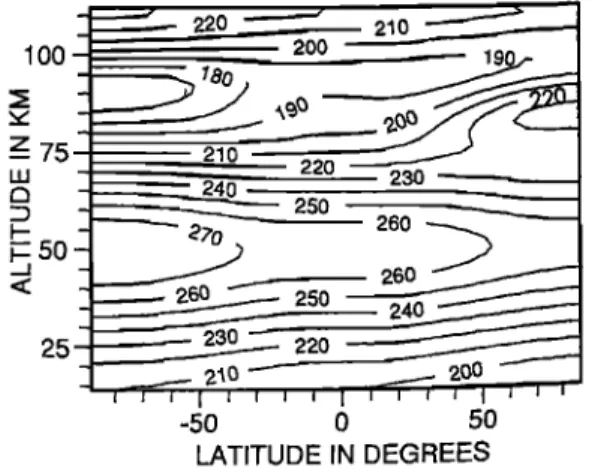
no gravity waves; a temperature profile is prescribed at the equator, thus giving the wind and temperature shown in figure 1 and figure 2 (we assume that we are under winter

' 'i ... I • I • ... •' • I I • ' • I I

-50 0 50

LATITUDE IN DEGREES

Fig. 1 ~ Initial zonal wind field (m/s).

lOO

z 75

25

-50 0 50

LATITUDE IN DEGREES Fig. 2- Initial temperature field (K).

conditions in the Northern Hemisphere); note the winter mesopause, colder than the summer one.

As the model runs the wave breaking progressively

produces

a realistic

inversion

of the meridional

gradient

.of

(figure

3), associated

with

the

formation

of realistic

jets

in

mesosphere,

i.e. westerly

winds

in the Northern

H .•ere

(winter)

and easterly

winds

in the Southern

Hemisphere

(summer)

(figure.4).

Furthermore

a temperature

inversim

100-•- .. -.. -

2oo,----

o _1

255

Fig.

3 - Temperathe

field

(K) •ter 15

days

in •e refem•

Hauchecorne and Maillard: 2-D model of mesospheric temperature inversions 2199

too

-

•50

Z

25-

Fig.

4 - Zonal

wind

field

(m/s)

after

15 days

in the

reference

simulation.

layer

is generated

in the

altitude

range

75-85

km between

50

rare

profile

at 60 øN Iatimde

(figure

5) shows

the

development

spheric

temperature

inversion)

below

the

mesopause,

with

a

wSth this inversion (figure 6) is localized in the mesospheric

region

above

75 km altitude,

which

is 15 lart higher

than

in

In order to understand which are the most important

physical

processes

in the

formation

of temperature

inversions,

a series of tests has been made.

First the model was tested with only one wave. The only kind of wave able to produce heating in the Northern Hemisphere must have a zero or negative phase speed. Of

course there is no inversion of the mesospheric gradient of

temperature between the poles, since such waves cannot propagate in the summer hemisphere, but mesospheric inver-

sions occur in the Northern Hemisphere with phase speeds c

equal to 0 or to -20. The amplitude of the inversion is weaker

with only one wave, and is found stronger with c=-20 than

with c=0. The inversion also occurs when five waves are in-

chded

with

phase

speeds

c=-30,

-15, 0, 15 and

30 ms

-1.

modynamical equation (3) each term was suppressed altema-

fiYely. The inversion layer is slightly weaker when the energy

120' 10•' 90' 75- 60'. 45' 15' 150 175 27,5 TEMPERATURE(K)

Hg.

5 - Evolution

of the

temperature

profile

at 60øN

latitude

thring

20 days

of simulation.

The

labels

indicate

the

day

of

corresponding

profile.

lOO

;5

% 5o

Fig. 6 - Drag (in m/s/day) after 10 days of simulation.

dissipation is suppressed and not significantly affected when

the turbulent diffusion is cut. If the NewtonJan cooling is

suppressed, the inversion also remains, but of course the mean temperature slowly increases at each altitude level. In contrast the inversion disappears completely when the adia- batic wamaing due to the vertical velocity is suppressed.

The thermal budget of the atmosphere has been made at 60 øN for the day 15 (figure 7) and confirms the previous analysis: the adiabatic heating is the most important term for

the formation of the warm layer and is partially compensated

by the Newtonian cooling in the altitude range where the in-

version occurs. The diffusion and the turbulent heating are clearly less important in this process.

1OO - _•75- r2:) - =2} - • - l-- ' _•50 --5 0 5

HEATING RATE IN K/DAY Fig. 7 - Thermal budget at 60øN latitude on day 15.

curve 1' Newtonian cooling.

curve 2: Potential temperature diffusion.

curve 3: tufi•ulent heating.

curve 4: adiabatic heating.

Another important factor in the formation of the inver-

sion is the narrowness of the layer of wave breaking. This

narrowness

is depending

on the value

of K (or • if N=N0)

breaking level is reached (u'=•-c). A simulation has been made with a v•ue of K equal to 1.2 ms-1 instead of 0.6 ms-l,

similar to •e • values used i.n Holton [1982, !983] ranging from 1.2 to 2 ms 'l. The resulting temperature field obtained

after 15 days (figure 8) shows a result simil• to previous 2D

2200

_Hauchecorne

_{and Maillard:}

_{2-D model}

_{of mesospheric}

_temperature

_inversions

22.•

. .20•

100• ' o ' "---'-'

',e' 17•_•_

, ,•_•

½'-'1

--

250

!.--

50

•

•o

Fig. 8 - Temperature field (K) obtained with K=l.2 ms -1 after

15 days of simulation.

warm at winter pole but without temperature inversion. Note

that a value of 1.6 ms -1 for K produces an amplitude for the

wave of the order of 45 ms -1 if this wave breaks at 70 km, which is probably too large. A smaller value for K is

therefore certainly more realistic.

Discussion and conclusion

This study shows that a 2-D dynamical model, taking into account the drag, diffusion and dissipation due to gravity wave breaking, is able to produce the formation of a stable mesospheric inversion of temperature in winter. The main mechanism that produces this layer is an adiabatic warming associated to downward mean vertical velocities of the order

of 1 to 2 cms 4 in the region 75-85 km. This vertical velocity

is in the same order than in previous models [e.g. Holton,

1983]. The only difference is that in our case the wave

breaking and then the strong downward motion are limited to the upper mesosphere. The narrowness of the layer of wave

breaking is a necessary condition for the formation of a tem- perature inversion.

Recent studies [Mcintyre, 1989] pointed out that the concept of eddy diffusivity might suffer some shortcomings in certain conditions and that some precautions should be taken in future models including wave drag parameterizations. A gravity wave parameterization such as the one presented in this paper probably overestimates the values of the diffusion, even with the value we choose for [• (0.3 instead of 1 in the original Lindzen parameterization). Strobe! et al. [ 1987] have shown from measurements of vertical constituent transport in

the mesosphere that the eddy Prandd number Pr used to de- scribe the constituent and potential temperature diffusion must be of order 10 to explain the data, which corresponds to

[3=l/Pr=0.1. Nevertheless we have shown that even if we neglect the potential temperature diffusion, the inversion oc-

curs.

Though this first modelling of mesospheric inversions

is encouraging, two important questions remain. First, further

studies will' have to explain how mesospheric inversions are

able to occur at middle latitudes in the real atmosphere, which is pot the case in this model. The use of a 3-D model might

partially

answer

this

question.

One

idea

is that

a displacemere

of the jet, due

for example

to planetary

waves,

co•d

influence

the

location

of mesospheric

inversions.

A second

problem

is that summer

mesospheric

inversions

are

not

simulated

with

this

model;

these

inversions

are

more

spara•

in the

real

atmosphere

and

not

very

stable.

A 2-D

mech•ards•

model

with

a constant

source

of gravity

waves

is

probably

not

able to reproduce such summer inversions.

Acknowledgments:

the authors

wish

to thank

•

M.L.Chanin

for

her

helpful

comments

and

suggestions.

•

are

also

grateful

to Dr M.E.Mclntyre

who

made

stimulating

comments to improve this paper. References

Clancy, R. T. and D. W. Rusch, Climatology and trends mesospheric (58-90 km) temperatures based upon !982-

1986 SME limb scattering

profiles,

J. Geophys..

R__•

9__4_4, 3377-3393, 1989.

Ebel, A., Contributions of gravity waves to the mornentre,

heat

and

turbulent

energy

budget

of the

upper

mesosphere.

737, 1984.

Hauchecorne, A., M. L. Chanin and R. Wilson, Mesosopheric temperature inversion and gravity wave

breaking, Geophys. Res,.Letters., 14, 933-936, 1987. Holton, J. R., The role of gravity wave induced drag and

fusion in the momentum budget of the mesosphere, J_. A. tmos. Sci., 32, 791-799, 1982.

Holton, J. R., The influence of gravity wave breaking on ':the general circulation for the middle atmosphere, J Am

.Sci., 40, 2497-2507, 1983.

Lindzen, R. S., Turbulence and stress owing to gravity wave and tidal breakdown, J...Geophys. Res., 86, 9707-9714, 1981.

Mcintyre, M. E., On dynamics and transport near •e po•

mesopause in summer, J...Geophys. Res., 94, 14617-

14628, 1989.

Manson, A. H. and C. E. Meek, Gravity wave propag•aa characteristics (60-120 km) as determined by

Saskatoon MF Radar (Graynet) system: 1983-85 at 52•N,

107øW, J. Atmos. Sci., 45, 932-946, 1988.

Matsuno, T., A quasi one-dimensional model of the atmosphere circulation interacting with internal grav'.• waves, .J, Meteor. Soc-Japan, 60. 215-226, 1982.

Schmidlin, F. J., Temperature inversions near 75 .kin, Geophys. Res.•Letters, 3. 173-176, 1976.

Schoeberl, M. R., D. F. Strobe! and J.P. Apmzese, A

merical model of gravity wave breaking and stress in the mesosphere, J. Ge. ophys. Res., • 5249-5259, 1983. Strobel, D. A., M. E. Summers, R. M. Bevilacqua, M.

DeLand and M. Alien, Vertical constituent transport in mesosphere, J. G.e. ophys, Res,, 9_2., 6691-6698, 1987.

A. Hauchecorne and A. Maillard, Service d'Airon :• du CNRS, B.P.3, 91371 Verri•res-le-Buisson cidex, France.

(Received December 6, 1990;

revised June 1, 1990;