HAL Id: hal-00295375
https://hal.archives-ouvertes.fr/hal-00295375
Submitted on 9 Dec 2003
HAL is a multi-disciplinary open access
archive for the deposit and dissemination of
sci-entific research documents, whether they are
pub-lished or not. The documents may come from
teaching and research institutions in France or
abroad, or from public or private research centers.
L’archive ouverte pluridisciplinaire HAL, est
destinée au dépôt et à la diffusion de documents
scientifiques de niveau recherche, publiés ou non,
émanant des établissements d’enseignement et de
recherche français ou étrangers, des laboratoires
publics ou privés.
from five nordic background stations
P. Tunved, H.-C. Hansson, M. Kulmala, P. Aalto, Y. Viisanen, H. Karlsson,
A. Kristensson, E. Swietlicki, M. Dal Maso, J. Ström, et al.
To cite this version:
P. Tunved, H.-C. Hansson, M. Kulmala, P. Aalto, Y. Viisanen, et al.. One year boundary layer aerosol
size distribution data from five nordic background stations. Atmospheric Chemistry and Physics,
European Geosciences Union, 2003, 3 (6), pp.2183-2205. �hal-00295375�
Chemistry
and Physics
One year boundary layer aerosol size distribution data from five
nordic background stations
P. Tunved1, H.-C. Hansson1, M. Kulmala2, P. Aalto2, Y. Viisanen3, H. Karlsson1, A. Kristensson4, E. Swietlicki4, M. Dal Maso2, J. Str¨om1, and M. Komppula3
1Institute for Applied Environmental Research, Stockholm University, SE-106 91, Stockholm, Sweden 2Department of Physics, POB 9, FIN-00014 University of Helsinki, Finland
3Finnish Meteorological Institute, POB 503, FIN-00101 Helsinki, Finland 4Division of Nuclear Physics, POB 118, SE-221 00 Lund University, Sweden
Received: 29 January 2003 – Published in Atmos. Chem. Phys. Discuss.: 23 May 2003 Revised: 3 December 2003 – Accepted: 4 December 2003 – Published: 9 December 2003
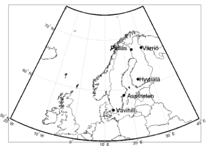
Abstract. Size distribution measurements performed at five different stations have been investigated during a one-year period between 01 June 2000 and 31 May 2001 with fo-cus on diurnal, seasonal and geographical differences of size distribution properties. The stations involved cover a large geographical area ranging from the Finnish Lapland (67◦N) down to southern Sweden (56◦N) in the order V¨arri¨o, Pallas,
Hyyti¨al¨a, Aspvreten and Vavihill. The shape of the size dis-tribution is typically bimodal during winter with a larger frac-tion of accumulafrac-tion mode particles compared to the other seasons. Highest Aitken mode concentration is found during summer and spring during the year of study. The maximum of nucleation events occur during the spring months at all sta-tions. Nucleation events occur during other months as well, although not as frequently. Large differences were found between different categories of stations. Northerly located stations such as Pallas and V¨arri¨o presented well-separated Aitken and accumulation modes, while the two modes often overlap significantly at the two southernmost stations Vavi-hill and Aspvreten.
A method to cluster trajectories was used to analyse the impact of long-range transport on the observed aerosol prop-erties. Clusters of trajectories arriving from the continent were clearly associated with size distributions shifted to-wards the accumulation mode. This feature was more pro-nounced the further south the station was located. Marine- or Arctic-type clusters were associated with large variability in the nuclei size ranges.
A quasi-lagrangian approach was used to investigate trans-port related changes in the aerosol properties. Typically, an increase in especially Aitken mode concentrations was ob-served when advection from the north occurs, i.e. allowing
Correspondence to: P. Tunved
more continental influence on the aerosol when comparing the different measurement sites. When trajectory clusters ar-rive to the stations from SW, a gradual decrease in number concentration is experienced in all modes as latitude of mea-surement site increases.
1 Introduction
Many processes in the atmosphere concerning aerosol parti-cles are closely related to the size distribution, and a well-developed understanding of the size distribution is required in order to evaluate the effect of aerosols on both climate and human health. The effect on climate is generally divided into a direct and indirect effect. The direct effect comes from the ability of aerosols to scatter and absorb incoming solar ra-diation, while the indirect effect is a result of the ability of aerosols as acting as cloud condensation nuclei (CCN) and thereby altering the radiative properties of clouds (Twomey, 1974). Also, health problems arising from particulates have been given a greater amount of interest during last years (K¨unzli et al., 2000).
Most size distribution measurements so far are over a lim-ited time period or only representative for a smaller area. Some work has been performed in this field, though. To be mentioned are recently published works by Birmili et al. (2001) that have sprung out with results that are useful for climatologically modelling. Birmili and co-workers (2001) found, when investigating the aerosol properties in Melpitz, typical size distribution attributable to the air mass where measured. Most pronounced differences were found between air masses of continental and marine origin, with a larger aerosol mass associated with air-masses of continental ori-gin.
Studies performed by Kulmala et al. (2000) have come up with similar results for the two Finnish stations V¨arri¨o and Hyyti¨al¨a. Winds from SW Russia and central Europe brought about far higher loads of accumulation particles as compared with those of arctic origin. Aitken mode was found to vary insignificantly when comparing the origin of air masses. Other long-term studies of the aerosol size distri-bution are reported from Jungfrauhoch (the Swiss Alps) with emphasis on air-mass origin (Nyeki et al., 1998).
The objective of this paper is to broaden the view of the Nordic aerosol in order to allow conclusions concerning the aerosol properties, i.e. find the seasonal variation for the whole Nordic region through the year of study and investi-gate how the aerosol varies over the region and establish a view on how long-distant transport effects different parts of the region. To achieve these goals 5 different stations ob-serving size distribution data on timescales of minutes are utilized. The study will focus on data collected during one year at these five stations located in Finland and Sweden, namely Aspvreten (Institute for Applied Environmental Re-search, Air Pollution Laboratory), Vavihill (Lund Univer-sity), Hyyti¨al¨a and V¨arri¨o (University of Helsinki) as well as Pallas (Finnish Meteorological Institute). In order to pro-duce results relevant for modelling and process studies, the conceptual model of lognormal fitting has been applied to the individual scans in order to reveal seasonal as well air-mass history related effects on the aerosol size distribution during the year of study. To fulfil the goal of presenting a dataset with both seasonal and spatial considerations, a clustering model presented by Dorling et al. (1992a, b), have been used to treat a large number of trajectories arriving at the indi-vidual stations. This will allow conclusions concerning the effect of source area on the aerosol studied.
2 Methods
2.1 Clustering model
Cluster analysis is a multivariate technique aiming to maxi-mize the variance between different groups and to minimaxi-mize the variance within a group of variables. A cluster analysis applied to trajectory data may be useful in order to recog-nize and quantify the influence of synoptic meteorology on the aerosol climatology. The trajectory data itself relies on trajectories calculated with the HYSPLIT4 (HYbrid Single-Particle Lagrangian Integrated Trajectory) model (Draxler and Hess, 1998). For this study 96 h back trajectories where calculated throughout the year for all stations at four times a day (UTC: 05, 11, 17, 23).
Since each individual trajectory is constructed from wind fields, they must reflect the evolution of a synoptic pat-tern during the 4 days they reach back in time. Dorling et al. (1992a) indicate how a composite surface pressure pattern representing an ensemble of trajectories reveals typical
atmo-spheric circulation features resulting in the transport patterns represented by the individual trajectories. When linking the cluster analysis to the actual size distribution measurements this will prove important. The evolution of the size distri-bution during a couple of days is strongly dependent on the weather situation and not only the source areas. Notably, cloud processing and washout by precipitation is of crucial importance. In order to make inter-comparisons between the different stations, it is therefore preferential to try to find and evaluate situations when similar meteorological history ap-plies to the air mass measured in. Since the clustering pro-cedure roughly will represent some typical weather situation we will be able to reduce the bias of the size distribution re-sulting from meteorological variations during the transport, as compared with cases if we choose only to look at the air mass origin in terms of sectors. This will allow us to inves-tigate effects from transport in-between stations, finding the important differences resulting from factors acting upon the size distribution during transport.
The clustering method utilized for these purposes is an ap-proach suggested and thoroughly described by Dorling et al. (1992a, b).
2.2 Model for aerosol size distribution
In order to allow comparisons between size distributions col-lected within different clusters as well as size distributions collected at different sites some general assumption has to be done concerning the size distribution. An often applied ap-proach is the use of relatively simple equations to describe the aerosol size distribution as separated in one or more distinct modes, i.e. the lognormal aerosol size distribution (Whitby, 1978; Hoppel et al., 1994). This allows straight-forward comparisons of the data between different stations by means of a set of well-defined parameters. This approach is well treated in the literature and the overall outcome has proved useful when parameterisations are required (e.g. Bir-mili et al., 2001; M¨akel¨a et al., 2000a).
In this study the aerosol size distribution has been inter-preted in terms of three modes, nuclei (<30 nm), Aitken (30– 110 nm) and accumulation mode (110–1000 nm). These modes are closely related to the processes leading to their appearance. Nuclei mode particles may be formed from con-densing gases if some critical concentration is reached. This nucleation phenomenon has been extensively treated in the literature (e.g. Kulmala et al., 2001; V¨akev¨a et al., 2000; Kulmala et al., 1998).
The lifetime of freshly formed particles is short, because of the growth by condensation but mostly due to removal by coagulation with larger particles. Coagulation between cleation mode particles and condensation of gases onto nu-clei mode particles constitute growth mechanisms of nunu-clei mode into the Aitken mode size range. While this growth by condensation and self-coagulation of nuclei mode particles leads to increased number concentration in the Aitken mode,
Table 1. Boundaries used as input for the automated fitting procedure for size distribution with three modes. Geometrical mean diameter
(Dg), geometrical standard deviation (GSD) and number concentration (N) limits are used. Number concentrations between zero-infinity are allowed. Modal diameters may overlap.
N1 (# cm−3) GSD1 Dg1 (nm) N2 (# cm−3) GSD2 Dg2 (nm) N3 (# cm−3) GSD3 Dg3(nm)
Lower boundaries 0 1.1 Smallest size of instrument 0 1.1 20 0 1.1 80
Upper boundaries ∞ 1.8 60 ∞ 2.0 120 ∞ 2.0 Largest size of instrument
coagulation with larger particles might serve as a significant sink for newly formed nuclei mode particles. Transformation of nuclei mode particle mass into Aitken mode mass seems to largely be controlled by direct coagulation between nu-clei mode particles and Aitken mode particles without ob-served growth of the actual nuclei mode.. Transformation of nuclei mode particle mass into Aitken mode mass seems to largely be controlled by direct coagulation between these particles without observed growth of the actual nuclei mode. This would only lead to an increased mass in the Aitken size ranges, leaving the number concentration unaffected. Only situations with favourable conditions (e.g. large nucleation rate and/or small coagulation sink) will lead to an observ-able growth of nuclei mode particles into the Aitken size ranges, thereby affecting their number concentration (Ker-minen et al., 2001). Otherwise, in order to maintain the num-ber concentration in the Aitken size ranges, direct emissions are required. In the literature it is argued that the primary emissions from anthropogenic activities largely contribute to aerosols in the Aitken size ranges (Birmili et al., 2001). Coarse mode particles may, if high enough concentration is present, serve as a significant sink of nucleation mode and Aitken mode particles. However, since coarse mode includes particles >1 µm (Seinfeldt and Pandis, 1998), no evaluation of this mode can be done due to instrumental limitations. The instruments used typically cover a size range from <10 nm to 500 nm.
Subsequent growth into larger size classes requires a large amount of condensing gases. The most important mechanism transforming Aitken mode particles into accumulation mode particles is cloud processing of the aerosol. Theoretically, this will produce well-defined modes with a pronounced min-imum in between, i.e. the Hoppel minima (Hoppel et al., 1994).
Since the goal was to fit each scan separately, some au-tomated fitting procedure had to be developed, taking into account the huge amount of data produced by five stations during one year. In order to produce results with a physical relevance, some constrains had to be supplied to the fitting routine. For this purpose restrictions concerning the geo-metrical standard deviation (GSD) and mean modal diameter (Dg) given in Table 1 were used.
The fitting procedure is performed with a Matlab® rou-tine involving two functions supplied with the Matlab® Op-timization Toolbox: LSQNONLIN for a first crude fit and FMINCON for the final fitting. LSQNONLIN starts with a
first crude approximation concerning modal diameters and number concentration. The output from this first fit serves as first guesses in FMINCON which performs a constrained fit with boundaries as described in Table 1. However, since the number of mathematical solutions to the lognormal function is large, additional constraints have to be applied, especially to avoid super-positioning of modes, which is mathemati-cally sound, but does not contribute with any useful informa-tion for this study. No modes are therefore allowed to have a spacing less than dlogDg<0.15, which roughly corresponds to a ratio of Dg’s>1.4. If a sound solution is not found within four iterations, a fitting with two modes is suggested. If the solution for two modes is not found within three attempts, fitting with one mode concludes the fitting procedure. This generally results in two modes, one in the Aitken and one in the accumulation size range, but appearance of a third mode occurs frequently, many times indicating new particle forma-tion . The presence of this third mode is generally confined to midday, indicating the importance of photochemistry in production of nuclei mode particles. However, it should be pointed out that this third mode is not always a nuclei mode, but can be a second Aitken or accumulation mode.
In order to understand this convention we have to be aware of the fact that the nature of the processes contributing to the different modes is not to be considered as discrete, but rather a continuous process. For example we can consider the growth of the nuclei mode due to condensation into the Aitken size range. If an Aitken mode already is present, which of course is the normal case, this growth would lead to appearance of two modes in the Aitken size range. Since smaller particles grow faster (by size) than larger, the two modes would in due time appear as one in terms of physical size distribution properties. In order to take similar situations into account it is necessary to include a term for this growing mode. In the following we thus include the term Aitken 1 and Aitken 2, where Aitken 2 is referred to as the semi-persistent Aitken mode and Aitken 1 denotes the growing mode.
Only very seldom we were able to resolve more than one mode in the accumulation mode size range so this type of definition is limited to the Aitken mode only. Fitting of three modes to the aerosol size distribution is of course an over-simplification. Four or even five modes may also be present as reported by Birmili et al. (1998) and Birmili et al. (2001), and this is not considered in our analysis. However, as shown in Sect. 3.4, three modes are sufficient to reproduce the mea-sured size distribution in this dataset.
Fig. 1. Location of the stations involved in the study.
2.3 Description of the stations 2.3.1 Hyyti¨al¨a
The background station Hyyti¨al¨a (61◦510N 24◦170E, 180 m a.s.l.) have been in focus in a number of large studies, especially concerning nucleation and new particle formation (e.g. M¨akel¨a et al., 2000; Nilsson et al., 2001a, b; Kulmala et al., 1998; Kulmala et al., 2001). The station, SMEAR II, (Station for Measuring forest Ecosystem-Atmosphere Rela-tions) is characterized as a boreal forest site, with surround-ings dominated by a flora of Scots Pine of about 30 years age. The station is located fairly far from urban pollution sites (Tampere at a distance of ∼50 km SW and Jyv¨askyl¨a
∼100 km NE). The station has facilitated particle size dis-tribution measurements since 1996, which have resulted in an extensive database including continuous measurement for over five years.
The instrument set-up consists of two differential mobility analyser systems, producing overlapping size distributions. The sample flow is split into two Vienna type differential mo-bility analysers (DMA). Two condensation particle counters (CPC) are used to detect the selected particles, one Model 3010 from TSI and one Model 3025 from TSI. The compos-ite instrument set-up produces size distributions between 3– 25 nm overlapping with a size distribution spectrum covering the range 20–500 nm. A full size scan is produced every 10 minutes.
2.3.2 V¨arri¨o
The SMEAR I station (67◦460N 29◦350E, 400 m a.s.l.) in V¨arri¨o is also classified as a background station and situated in the same vegetation as Hyyti¨al¨a (in this case a 40 year old Scots Pine forest). The station itself is located at a hill cap. The station is far from any pollution sources, although emis-sions on the Kola Peninsula give rather strong signals when winds are transporting air from this region (Kulmala et al.,
2000). Also, winds coming from the St. Petersburg area as well as Russia in general may bring elevated concentrations of acidifying gases as well as particulate pollution. The Dif-ferential Mobility Particle Sizer (DMPS) system set-up pro-duces a complete size scan between 8 and 460 nm approx-imately every 10 min. Aerosol concentrations are generally low, on average somewhere in the order of 500 particles per cubic centimetre.
2.3.3 Pallas
The Matorova station at Pallas (68◦000N 24◦140E, 340 m a.s.l.) is located in the depths of the sub arctic pine forest in the Pallas – Ounastunturi National Park that spans over 50000 hectares. The particle measurements are made by Finnish Meteorological Institute (FMI) and the station it-self is a part of the Global Atmospheric Watch (GAW) pro-gramme. The proximity to the V¨arri¨o station allows a good basis for comparison between these stations when simultane-ous measurements are performed. DMPS-system set-up con-sists of one medium DMA separating the particles according to size, subsequently detected by a 3010 CPC from TSI. Size distributions between ∼7–490 nm are observed with this set-up.
2.3.4 Aspvreten
The background station Aspvreten (58◦800N, 17◦400E, 25 m a.s.l.), is located in S¨ormland, some 70 km south west of Stockholm. The station is situated about 2 km from the coast in a rural area covered by mixed coniferous and decid-uous forest with some meadows. The influence from anthro-pogenic activities is small, and the area around the station is sparsely populated. The station is operated by the Institute for Applied Environmental Research, Air Pollution Labora-tory, and is a part of the European Monitoring and Evaluation Programme network (EMEP). The instrumental set up on the station, besides meteorology and PM 2.5/10 measurements, consist of a medium DMA along with a TSI 3010 CPC. The instrument set-up observes one size distribution spectrum ev-ery 6 min in the size ranges 10–452 nm.
2.3.5 Vavihill
Vavihill (56◦010N, 13◦090E, 172 m a.s.l.) is a background station at the top of S¨oder˚asen in Sk˚ane. The surroundings are dominated by grasslands and deciduous forest. The sta-tion is situated about 10 km away from the closest small vil-lages and about 20 km from the city Helsingborg. The area of Malm¨o and Copenhagen, with about 2 million inhabitants is situated about 60–70 km to the SSW. However it is not con-sidered to be influenced by local anthropogenic activities and has facilitated background monitoring measurements since 1984. The station is mainly influenced by SW winds. The in-strument set-up consists of two differential mobility analyser systems (Ultrafine Differential Mobility Analyser (UDMA)
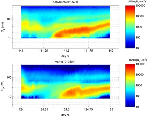
Fig. 2. Example of typical nucleation events at Aspvreten (upper frame) and V¨arri¨o (lower frame).
and Differential Mobility Analyser (DMA), respectively). The separated particles are detected by a TSI CPC 3025 for sizes 3.1–22 nm and one TSI CPC 7610 detecting particles 22–∼900 nm. During the year of study, measurements at Vavihill only covers a portion of the winter and spring pe-riod (February–April 2001). Therefore no seasonal variation can be evaluated with this data. Locations of the stations are displayed in Fig. 1.
3 Results
3.1 Diurnal variation
The diurnal behaviour of the aerosol at the different stations has been investigated. Mainly to reveal any local sources influence on the measurement. No indications of local an-thropogenic influence were found. Nucleation events were observed at all stations. These occasions are typically char-acterized by a sharp increase of nuclei mode number concen-tration around noon. During this year of study, the frequency of the nucleation events has been shown to be largest around springtime, between March–May. This seasonal variation in nucleation frequency has been observed at Hyyti¨al¨a earlier (e.g. Kulmala et al 2001, M¨akel¨a et al., 2000b, Nilsson et al., 2001).
Figure 2 shows example of typical events at the measure-ment stations Aspvreten and V¨arri¨o, revealing the commonly
Table 2. Growth rate and peak concentration during class 1 events
at the different stations. Number of events meeting criteria is also given in table during the year of investigation.
GR(nm/h) Nmax # class 1 events
Aspvreten 2.3 9661 17
Hyyti¨al¨a 1.9 7649 22
Pallas 1.6 3047 17
V¨arri¨o 2.0 2571 25
observed characteristics of the nucleation phenomenon. The fact that we are able to follow the growth for several hours in-dicates that the phenomenon occurs on a large spatial scale. Nucleation has earlier been reported to occur during sunny days (Kulmala et al., 2001). Further it was in the present study concluded that nucleation occur in air arriving from N/NW in most of the cases. Nucleation as shown in Fig. 2 is only very seldom observed in air advected from S/SE. Ear-lier reports stretch the importance of cold air advection and boundary layer height (e.g. Nilsson et al 2001). Also, high concentration of pre-existing aerosol is believed to quench the nucleation due to large condensational and coagulation sink, due to removal of the precursor gases and initially formed cluster respectively.
In Table 2 statistics of the observed nucleation events dur-ing the year of study is summarized. In this statistics we
1 10 100 1000 0 1000 2000 3000 4000 5000
Days with no nucleation
D p (nm) dN/dlogD p (cm −3 ) 0−4 4−8 8−12 12−16 16−20 20−24 1 10 100 1000 0 1000 2000 3000 4000 5000
Days with nucleation
D p (nm) dN/dlogD p (cm − 3) 0−4 4−8 8−12 12−16 16−20 20−24
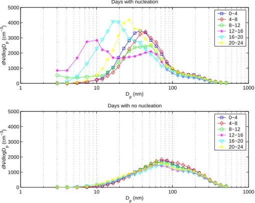
Fig. 3. Time dependent evolution of the size distribution during March–May. Each plot represents the average during four hours intervals
for the whole season. Upper frame shows days with nucleation and lower frame median of days with no nucleation.
only include the most pronounced events following a defini-tion by M¨akel¨a et al. (2000b). The growth rate was found to be largest at Aspvreten, by 2.3 nm/h. Peak concentra-tions observed during the events was highest at Aspvreten (∼9600 cm−3 on average) and lowest at V¨arri¨o and Pallas.
Thus both growth rate and number concentration of newly formed particles is highest at Aspvreten.
The diurnal variability in the shape of the size distribution was investigated. In Fig. 3 the composite time dependent median size distributions for Hyyti¨al¨a during March-May are depicted. The data have been divided into 4 h intervals and calculated as the median of the integral of scans during the period of the year.
The data was further divided into one sub-set with days with typical nucleation events and another with days when we did not observe nucleation events. Two features become obvious. First, a systematic diurnal variation is only ob-served for the sub-set with nucleation. In the case with nucle-ation events we experience this as an initial increase of small particle in the time interval between 08:00–12:00, even more pronounced during 12:00–16:00. Hereafter the size is shifted towards larger particles during time-steps 16:00–20:00 and 20:00–24:00. This behaviour could be interpreted as growth of the small, initially formed, particles. This since we be-lieve that the nucleation phenomena can be observed over large areas simultaneously. We cannot observe a systematic diurnal variation in the sub-set with no nucleation. The
sec-ond feature comparing the behaviour of the two data sets is the fact that the nucleation sub-set has obviously much less mass associated with the aerosol as compared with the non-nucleating cases (e.g. much larger number concentration in the accumulation mode size range in non-nucleation cases as compared with nucleation cases). This probably reflects the fact that we observe nucleation when we have northerly advection, which is likely to bring rather clean air to the mea-surement sites.
This typical features comparing statistics concerning non-nucleation days and non-nucleation days are found at all stations. That is, nucleation events do affect the size distribution in a diurnal fashion. This feature is lacking for non-nucleation days.
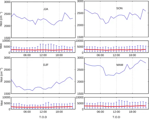
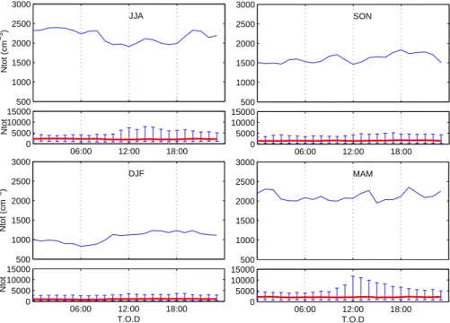
The diurnal variation of the integral number per season has also been investigated. In Fig. 4 the results for Aspvreten are given. The data is presented as 1h median concentra-tion for the season studied. Only small, if any, diurnal varia-tion in integral number is found. The variavaria-tions encountered are typically in the range ±10%. 5–95 percentiles are in-dicated below each plot, showing occasions with maximum number concentration. The highest concentrations, shown by the 95 percentile, do occur during daytime.
Most probably, these peaks in integral number concentra-tion can be attributed to nucleaconcentra-tion events, treated in previous section. These peaks are furthermore confined to summer and spring periods of the year, which is in nice agreement
1500 2000 2500 3000 Ntot (cm −3 ) JJA 06:00 12:00 18:00 0 5000 10000 Ntot 1500 2000 2500 3000 SON 06:00 12:00 18:00 0 5000 10000 1500 2000 2500 3000 Ntot (cm − 3) DJF 06:00 12:00 18:00 0 5000 10000 Ntot T.O.D 1500 2000 2500 3000 MAM 06:00 12:00 18:00 0 5000 10000 T.O.D
Fig. 4. Diurnal variation of median integral number concentration per season, June–August (JJA), September–November (SON), December–
February (DJF) and March–May (MAM) at Aspvreten. Indicated in subplots are 5th-95th percentiles. T.O.D. denotes time of day. Note that
the axis scale for the number density begins at 1500 cm−3for the large frames.
with the nucleation inventory established for the different sta-tions.
Figure 5 describes the diurnal variability of integral num-ber recorded at Hyyti¨al¨a. In comparison with the Aspvreten dataset, even less pronounced variations for the Hyyti¨al¨a data was observed. Largest variations are encountered during summer and autumn, however still below ±10%. Neither the winter nor summer median integral number data can be ad-dressed with any diurnal variation. However, investigating the 5–95 percentile ranges, occasions with maximum con-centrations are shown to occur during daytime. This espe-cially applies during spring and summer, but same tendencies can be observed during autumn.
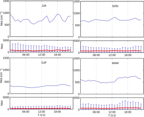
Performing the same analysis for V¨arri¨o we find only small tendencies to diurnal behaviour for all seasons (Fig. 6). The 95 percentile shows no or weak diurnal variation for all seasons except the spring period, when occasions with very high integral number concentration can be observed dur-ing noon. Smallest variations are encountered durdur-ing winter months December, January and February (DJF). Overall low-est concentrations are found during autumn and winter dur-ing this year.
Turning the attention to Pallas (Fig. 7), similar behaviour as for V¨arri¨o is observed. Only weak diurnal variations seem to be present. No diurnal behaviour can be addressed to the winter season.
Conclusively, the diurnal variations of the integral num-ber encountered at the stations are small, typically below
±10%. This reduces the possibility that the aerosol is af-fected by local sources. The nature of industry and house-hold activities in the vicinity of the stations typically follows a diurnal pattern (e.g. lack of large industries with 24 h pro-duction activity). Thus if local anthropogenic activities do affect the aerosol size distribution, this would be evident as diurnal variation of the aerosol number concentration. Fur-thermore, nucleation events seem to affect the integral num-ber concentration for at least Aspvreten and Hyyti¨al¨a in a diurnal fashion when investigating the 95 percentile of the dataset. These trends are not equally obvious for the V¨arri¨o and Pallas datasets. However, the events occur as frequent at these stations as observed for e.g. Hyyti¨al¨a during this year of study. Although we do not see any large diurnal varia-tions in the integral number we do observe typical diurnal changes concerning the shape of the size distribution. This is most obvious during spring and is attributed to new particle formation events.
3.2 Variation of aerosol properties between the seasons of the year of measurement
In Figs. 8–11 the seasonal features of the aerosol size distri-bution found during the year of study are depicted as median size distribution per season. The data have been cleaned from
500 1000 1500 2000 2500 3000 Ntot (cm −3 ) JJA 06:00 12:00 18:00 0 5000 10000 15000 Ntot 500 1000 1500 2000 2500 3000 SON 06:00 12:00 18:00 0 5000 10000 15000 500 1000 1500 2000 2500 3000 Ntot (cm − 3) DJF 06:00 12:00 18:00 0 5000 10000 15000 Ntot T.O.D 500 1000 1500 2000 2500 3000 MAM 06:00 12:00 18:00 0 5000 10000 15000 T.O.D
Fig. 5. Diurnal variation of median integral number concentration per season, June–August (JJA), September–November (SON), December–
February (DJF) and March–May (MAM) at Hyyti¨al¨a. Indicated in subplots are 5–95 percentiles. T.O.D. denotes time of day. Note that the
axis scale for the number density begins at 500 cm−3for the large frames.
0 500 1000 1500 Ntot (cm −3 ) JJA 06:00 12:00 18:00 0 5000 Ntot 0 500 1000 1500 SON 06:00 12:00 18:00 0 5000 0 500 1000 1500 Ntot (cm − 3) DJF 06:00 12:00 18:00 0 5000 Ntot T.O.D 0 500 1000 1500 MAM 06:00 12:00 18:00 0 5000 T.O.D
Fig. 6. Diurnal variation of median integral number concentration per season, June–August (JJA), September–November (SON), December–
February (DJF) and March–May (MAM) season at V¨arri¨o. Indicated in subplots are 5–95 percentiles. T.O.D. denotes time of day.
occasions indicating failure of the measurements. For each station and season, the resulting median has been lognormal fitted in three modes. The parameters are summarized in Ta-ble 3.
A nucleation day inventory has been established per sea-son for all stations. Nucleation data is grouped follow-ing a scale from 0–3 where 1 indicates most pronounced event when growth can be observed for several hours. Event
0 500 1000 1500 Ntot (cm −3 ) JJA 06:00 12:00 18:00 0 5000 Ntot 0 500 1000 1500 SON 06:00 12:00 18:00 0 5000 0 500 1000 1500 Ntot (cm − 3) DJF 06:00 12:00 18:00 0 5000 Ntot T.O.D 0 500 1000 1500 MAM 06:00 12:00 18:00 0 5000 T.O.D
Fig. 7. Diurnal variation of median integral number concentration per season, June–August (JJA), September–November (SON), December–
February (DJF) and March–May (MAM) at Pallas. Indicated in subplots are 5–95 percentiles. T.O.D. denotes time of day.
Table 3. Modal parameters obtained from fitting of the median size distributions per season for each station. Also the frequency of nucleation
events is presented.Here given as % days of the data set exhibiting nucleation as described under Sect. 3.1.
Station Season N1 (# cm−3) DSG1 Dg1 (µm) N2 (# cm−3) DSG2 Dg2 (µm) N3 (# cm3) DSG3 Dg3 (µm) % Nucl.days
Pallas Jun–Aug 93 1.71 0.029 282 1.49 0.053 115 1.44 0.182 10 Sep–Nov 69 1.69 0.036 179 1.43 0.074 230 1.61 0.160 2 Dec–Feb – – – 152 1.85 0.053 123 1.48 0.212 2 Mar–May 63 1.54 0.019 157 1.52 0.043 162 1.61 0.168 23 V¨arri¨o Jun–Aug 103 1.51 0.043 541 1.60 0.085 141 1.47 0.191 6 Sep–Nov – – – 263 1.82 0.073 112 1.46 0.200 7 Dec–Feb – – – 108 1.54 0.048 201 1.63 0.175 12 Mar–May 119 1.53 0.028 111 1.30 0.050 266 1.73 0.143 27 Hyyti¨al¨a Jun–Aug 429 1.66 0.034 887 1.58 0.077 327 1.46 0.192 7 Sep–Nov 227 1.63 0.025 776 1.62 0.068 295 1.44 0.200 7 Dec–Feb 204 1.80 0.025 389 1.62 0.061 270 1.48 0.200 0 Mar–May 431 1.74 0.025 849 1.69 0.067 284 1.44 0.200 25 Aspvreten Jun–Aug 250 1.62 0.035 1178 1.49 0.078 423 1.51 0.205 10 Sep–Nov 272 1.69 0.035 1429 1.61 0.071 494 1.47 0.220 7 Dec–Feb 431 1.80 0.026 917 1.75 0.066 377 1.46 0.217 2 Mar–May 507 1.73 0.033 1319 1.69 0.066 256 1.44 0.217 14
classes 2–3 do not show as pronounced growth as class 1. 0 represent occurrence of small particles, but no following growth is observed (M¨akel¨a, 2000b). In Table 3 class 1 & 2 events are considered. It should be pointed out that these
events do not appear in the median values of size distribu-tion since they are smoothed out by the large amount of data present.
10 100 500 0 1000 2000 3000 4000 5000 dN/dlogD p (cm −3 ) Jun−Aug % event days (1−2): 9.8% 10 100 500 0 1000 2000 3000 4000 5000 dN/dlogD p (cm − 3) Sep−Nov % event days (1−2): 6.6% 10 100 500 0 1000 2000 3000 4000 5000 dN/dlogD p (cm − 3) Dec−Feb % event days (1−2): 2.3% D P (nm) 10 100 500 0 1000 2000 3000 4000 5000 D P (nm) dN/dlogD p (cm − 3) Mar−May % event days (1−2): 14.1%
Fig. 8. Seasonal variation of median size distribution at Aspvreten (58.8 N, 17.4 E). Error bars indicate 25–75 percentile range. Different
modes from lognormal fitting appear in dashed, solid and dotted curves. % nucleation days indicated in upper left corner.
10 100 500 0 1000 2000 3000 4000 dN/dlogD p (cm −3 ) Jun−Aug % event days (1−2): 7% 10 100 500 0 1000 2000 3000 4000 dN/dlogD p (cm − 3) Sep−Nov % event days (1−2): 6.8% 10 100 500 0 1000 2000 3000 4000 D P (nm) dN/dlogD p (cm − 3) Dec−Feb % event days (1−2): 0 10 100 500 0 1000 2000 3000 4000 D P (nm) dN/dlogD p (cm − 3) Mar−May % event days(1−2): 24.6%
Fig. 9. Seasonal variation of median size distribution at Hyyti¨al¨a (61.51 N, 24.17 E). Error bars indicate 25–75 percentile range. Different
modes from lognormal fitting appear in dashed, solid and dotted curves. % nucleation days indicated in upper left corner.
The seasonal characteristics for Aspvreten and Hyyti¨al¨a are quite similar as seen in Figs. 8 and 9. The median size distribution for the summer (June–August) and spring (March–May) period both show rather high concentration in
the Aitken size ranges. The relative contribution of the ac-cumulation mode is largest during winter. The overall low-est concentrations are encountered during the winter period, and the Aitken and accumulation mode are separated to a
10 100 500 0 500 1000 1500 2000 2500 dN/dlogD p (cm −3 ) Jun−Aug % event days (1−2): 6.4% 10 100 500 0 500 1000 1500 2000 2500 dN/dlogD p (cm − 3) Sep−Nov % event days (2−3): 6.6% 10 100 500 0 500 1000 1500 2000 2500 D P (nm) dN/dlogD p (cm − 3) Dec−Feb % event days (1−2): 12.3% 10 100 500 0 500 1000 1500 2000 2500 D P (nm) dN/dlogD p (cm − 3) Mar−May % event days (1−2): 27.1%
Fig. 10. Seasonal variation of median size distribution at V¨arri¨o (67.46 N, 29.35 E). Error bars indicate 25–75 percentile range. Different
modes from lognormal fitting appear in dashed, solid and dotted curves. % nucleation days indicated in upper left corner.
larger extent compared to the other seasons. The frequency of nucleation is largest during spring months, but some nu-cleation bursts where encountered during the summer and autumn months. At Aspvreten we observed the lowest fre-quency of nucleation events during winter and autumn (see Table 3, DJF period).
For V¨arri¨o, the overall largest concentrations are encoun-tered during summer (see Fig. 10). The larger number con-centration during the summer months is largely explained by an increase of particles in the Aitken size ranges. For all other seasons, the contribution from the accumulation and Aitken mode is found to be almost equal. A more or less pro-nounced minimum between the two modes is present during all seasons except summer. It is found as for the other sta-tions that the maximum frequency of nucleation days is en-countered during the spring period (March–May). However, a fairly high percentage of nucleation days were recorded at V¨arri¨o during the winter. This might be indicative of the closeness to smelters located at the Kola Peninsula. Easterly winds may bring elevated concentrations of nucleating gases or precursors thereof to the station from the smelters con-tributing to the observed nucleation. The seasonal pattern recorded at Pallas is similar to that at V¨arri¨o (see Fig. 11). Largest integral number concentrations are encountered dur-ing summer. However, there is a distinct minimum between accumulation and Aitken mode present during the summer months. The maximum in nucleation days occur during spring.
Unfortunately, the Vavihill station could not contribute with enough data to support a seasonal analysis. Data avail-able from the station only covers February–April 2001.
Obviously there is a gradient in integral number when comparing the northernmost stations with the southerly lo-cated ones, with maximum aerosol concentrations found at Aspvreten. Although sparse in data, Vavihill tends to show equally high or higher aerosol concentrations as compared with Aspvreten. .
It is also obvious that the largest frequency of nucleation is confined to the spring period (MAM), although nucleation does occur both during summer and autumn, but more sel-dom (Table 3).
The maximum in integral number concentration is con-fined to the spring and summer months. This becomes obvious when investigating the daily mean concentration recorded for each station as presented if Fig. 12.
Potential explanations for this might be seasonal changes in air masses, lower rate of incoming solar radiation and thus less new particle formation during the winter period and/or a higher rate of precipitation and overall cloudiness during the winter.
3.3 Variation of trajectory orientation between the seasons of the year of measurement
In order to clarify the seasonal differences in typical advec-tion schemes as well as inter-staadvec-tion related differences in air mass history we have chosen to interpret the seasonal
10 100 500 0 500 1000 1500 2000 dN/dlogD p (cm −3 ) Jun−Aug % event days (1−2): 10% 10 100 500 0 500 1000 1500 2000 dN/dlogD p (cm − 3 ) Sep−Nov % event days (1−2): 2.1% 10 100 500 0 500 1000 1500 2000 D P (nm) dN/dlogD p (cm − 3) Dec−Feb % event days (1−2): 2.2% 10 100 500 0 500 1000 1500 2000 D P (nm) dN/dlogD p (cm − 3 ) Mar−May % event days (1−2): 24%
Fig. 11. Seasonal variation of median size distribution at Pallas (67.58 N, 24.07 E). Error bars indicate 25–75 percentile range. Different
modes from lognormal fitting appear in dashed, solid and dotted curves. % Nucleation days indicated in upper left corner.
0 100 200 300 400 0 1000 2000 3000 4000 5000 6000 7000 N(cm −3 ) Hyytiälä 0 100 200 300 400 0 500 1000 1500 2000 2500 3000 Day of year N(cm − 3) Värriö 0 100 200 300 400 0 500 1000 1500 2000 2500 3000 Day of year N(cm − 3) Pallas 0 100 200 300 400 0 1000 2000 3000 4000 5000 6000 7000 Aspvreten N(cm − 3)
Fig. 12. Daily mean integral concentration for stations V¨arri¨o, Pallas, Hyyti¨al¨a and Aspvreten (blue bars) and 7 days running mean (red line).
variation of preferred transport pathways to the stations by means of cumulative trajectory plots, each one specific for both season and station. A selection of these results is pre-sented in Fig. 13.
360 grid cells build up the plot. The colour of each cell represents the number of times a trajectory has passed through that specific grid cell during the season at hand.
Warm colours indicate that a large number for trajectories have crossed the grid cell. As an illustration we have chosen to compare the autumn and spring period between Aspvreten and V¨arri¨o.
Two features become obvious when studying the resulting plots. First, there is a strong seasonal variability in the orien-tation of the trajectories during the year of study. During the
Fig. 13. Seasonal variation in advection schemes. Above: The autumn and spring period for Aspvreten. Colour bar indicates cumulative
number of times a grid cell has been crossed by a trajectory. Below: Same as above, but for V¨arri¨o.
autumn period a large number trajectories arrive from S/SW. Thus, both stations are likely to experience the sources on the continent, changing the aerosol properties accordingly.” During spring the opposite applies, with trajectories arriving from the Arctic/marine environment dominating the trans-port to the different stations. The other feature is that for at least the spring period the two stations does not share the same advection pattern. The most dominant transport path-way to Aspvreten seems to be SE advection. Another im-portant pathway is SW. The trajectories arriving V¨arri¨o are preferentially arrive from NE. These features of the transport to the different stations somewhat limits the possibilities of making straightforward comparisons between the stations. It should be mentioned that both Hyyti¨al¨a and Aspvreten com-pares quite well in terms of seasonal variation of trajectory orientation, and that the largest differences are encountered when comparing these southerly located stations with V¨arri¨o and Pallas.
3.4 Linking clustering model with model for aerosol size distribution
In order to investigate transport related effects on the aerosol it is important to find situations when similar large-scale ad-vection situations apply to all stations studied. This will give us the opportunity to evaluate how the aerosol properties are changed, e.g. when the transport distance from the continent and its sources is increasing. Since the ensemble of stations
provides reference points with a good spatial coverage such an approach will clearly constitute a good basis for future modelling exercises.
In the following section we present an example of how the cluster analysis and the mode fitting model are linked. We have made use of the Finnish station Hyyti¨al¨a, where the data set has been divided into four seasons, June–August, September–November, December–February and March–May. A new set of clusters is calculated for each season. The clustering procedure will separate out trajec-tories whit air of similar meteorological history arriving to all receptor sites. The size distribution is evaluated as the scans collected during a period of two hours before and two hours after each trajectory arrival (local time). In order to as-sure stable conditions concerning trajectory orientation and thus similar pressure situation, situations showing large de-viations in trajectory orientation on time scales less than 12 h were filtered out.
The size distribution recorded around the arrival of all tra-jectories building the clusters is collected in this manner. Considering the timescale for the production of a new scan (minutes), this will give a large amount of size distribution data upon which the following analysis is built.
The resulting size distribution for three different cluster orientations arriving Hyyti¨al¨a during December to February 2000–2001 have been evaluated. The clusters resulting from the analysis is presented in Fig. 14.
Cluster B No of trajs 45
Fig. 14. Representation of trajectory clusters arriving Hyyti¨al¨a for the period Sep–Nov. The clusters are here presented as the mean of the
trajectories building the clusters. Numbers of trajectories in cluster are also indicated.
Table 4. Modal parameters as derived from lognormal aerosol model. 25-75th percentiles indicated. Data corresponds to clusters A, B and
C discussed above. Fractional representation of the mode itself is also indicated.
Nucleation Nucleation Aitken 1 Aitken 1 Aitken 2 Aitken 2 Accumulation Accumulation
mode 25–75% mode 25–75% mode 25–75% mode 25–75%
Median percentiles median percentiles median percentiles median percentiles
Cluster A N (# cm−3) 586 282–834 938 803–1595 729 523–1080 268 220–340 DSG 1.74 1.56–1.80 1.57 1.51–1.72 1.44 1.34–1.54 1.47 1.36–1.56 Dg (µm) 0.021 0.016–0.025 0.033 0.031–0.035 0.053 0.049–0.058 0.176 0.159–0.190 fraction 0.736 – 0.150 – 0.992 – 0.935 – Cluster B N (# cm−3) 241 139–386 153 97–266 828 535–1305 533 338–842 DSG 1.80 1.63–1.80 1.61 1.45–1.70 1.61 1.51–1.73 1.52 1.44–1.61 Dg (µm) 0.021 0.018–0.024 0.034 0.032–0.035 0.075 0.063–0.086 0.203 0.178–0.227 fraction 0.369 – 0.125 – 0.936 – 0.989 – Cluster C N (# cm−3) 1310 428–1755 664 350–1035 733 336–1560 136 93–216 DSG 1.48 1.38–1.63 1.39 1.28–1.47 1.45 1.31–1.60 1.41 1.31–1.52 Dg (µm) 0.016 0.009–0.024 0.034 0.031–0.035 0.045 0.037–0.052 0.170 0.152–0.221 fraction 0.540 – 0.155 – 0.868 – 0.675 –
The general finding during December–February is that the most dominant transport pathways is southerly oriented. One cluster arriving from north (C) with a total number of 15 tra-jectories, one from south-west (A) with a total of 12 tories and one arriving from south (B) made up by 45 trajec-tories are presented here.
The numbers of size distributions in the different clusters are 306, 251 and 816 respectively. Each size distribution scan, collected around the arrival of each individual trajec-tory constituting the cluster, has been treated separately by fitting the lognormal aerosol model to the data. In Fig. 15 the median and 25th-75th percentile ranges of the size
distri-butions observed in each cluster is shown. The median cal-culated on the lognormal mode fitting procedure is indicated with crosses in the figure. This result is derived from the me-dian of the sum of model-reproduced scans. It is found that in most cases the lognormal mode model is able to reproduce the median size distribution with good accuracy. Only small deviations are experienced for the data resulting from cluster number A, where the fitting of the nuclei mode seems to be lacking in some cases.
In Table 4 the modal parameters obtained from fitting are presented. It is found that the largest nuclei mode concen-tration is present within the data collected in the marine
10 100 0 500 1000 1500 2000 2500 3000 3500 D (nm) A (0.99203) dN/dlogD p (cm −3 ) 10 100 D (nm) B (0.97917) 10 100 D (nm) C (0.95425) 25−75% Data Fit
Fig. 15. Comparison of SW-cluster (left), S-cluster (middle) and N-cluster (right) resulting median size distribution. The red crosses show
results derived from the fitting routine. Fraction of total number of scans accounted for by the model is indicated within brackets above.
cluster C. Further, the modal diameter is comparatively small. The Aitken mode shows largest differences when comparing the geometrical mean diameter, Dg. Typically, continental cluster (e.g. B) show an Aitken mode shifted towards larges sizes. Accumulation mode is found to be present more seldom in the marine case (C) as compared with clusters A and B that are influenced from continental sources to a larger extent. Concentrations found in this size range are also typically lower for the marine aerosol. Smallest ac-cumulation mode diameters are found in the marine cluster (C). GSD’s obtained are also typically larger for continental air masses.
This brief presentation of the lognormal size distribution model reveals the most pronounced differences when com-paring clusters of different origin. The features presented above is found for all stations in most cases, putting con-fidence in both the cluster model as well as the simplified fitting methods used.
As a result of more large aerosols present in the continental clusters, these types of clusters also accommodate largest in-tegral aerosol volume (3–450 nm). However, small variations in number concentration are found when comparing different clusters (Table 5). In this and several other cases we even find a lower integral number concentration to be associated with continental clusters as compared to those of marine origin. During the year of study we were able to identify situations when all or at least several stations had resulting clusters with similar orientations. As argued in the chapter dealing with the clustering model, situations with similar ensembles of trajectories arriving to different stations will allow us to eval-uate the transport related changes with a reduced bias from meteorological variation. This since the trajectories roughly will represent the wind fields shaping the trajectories, and therefore the synoptic pressure situation. For this purpose
a number of interesting cases have been selected to put light on how the aerosol is affected when transport over the Nordic countries occurs. The most dominant transport pathway was found to be SW trajectories. This orientation found repre-sentation for all stations during all seasons. However, also situations when other advection schemes applied have been investigated in detail.
In addition to the pre-classification delivered by the fitting routine as described earlier, the data was interpreted accord-ing to followaccord-ing conventions: the nuclei mode is confined to the size ranges smallest bin size of instrument – 30 nm. Sec-ondly, contribution to Aitken 2 is made by particles in the 30–110 nm size ranges. If three modes are present, although the first one could not actually be referred to as nuclei mode but falls in the Aitken size range, this mode is called Aitken 1. The accumulation mode is made up by particles >110 nm. 3.4.1 Case I, NE clusters
In Figs. 16a and b two occasions with NE cluster to the dif-ferent station are shown. These situations occurred during the winter period (December–February, Fig. 16a) and spring period (Marc—May, Fig. 16b). During Dec-Feb V¨arri¨o, Pal-las, Hyyti¨al¨a and Aspvreten are represented. During the spring period also data from Vavihill were available, giving an opportunity to follow the aerosol in-between receptor sites widely separated. The number of trajectories building each cluster is given in the figures.
As discussed in Sect. 2.1, clusters will represent a typical synoptic weather situation. A comparison of similar clusters arriving different stations presents similar average pressure fields. In Fig. 17 average pressure fields are presented for the four stations involved in this case study. The averages were calculated over the four day duration of the individual
Fig. 16. NE clusters arriving to the different stations during Dec–Feb (a) and Mar–May (b). Clusters are represented as means. The time
spacing between each pair of endpoints (dots) in the figure is 5 h.
trajectories over the MAM-period (Fig. 16b). The different pressure fields present striking similarities as can be seen in the strong gradient over the North Sea and British Isles. The slight differences between the stations arise from the fact that the averages are calculated based on different days due to moving weather systems. This put confidence in the clus-tering procedure and actually confirms the idea that we will experience a reduced bias from station specific meteorology when comparing the different locations. Sea level pressure data was obtained from the NCEP/NCAR archives.
The resulting size distribution data for the NE-clusters is shown in Figs. 18a and b, both as median as well as the nor-malized distribution revealing the shape of the derived size distribution. When investigating the cluster data for the DJF-period we find ensembles of trajectories arriving from north-ern Russia. The mean clusters have the same source area in the beginning, but do split up in height with the Kola Penin-sula, where the air arriving to Aspvreten and Hyyti¨al¨a
con-tinue SW, while V¨arri¨o and Pallas clusters turn W. 27, 21, 13 and 17 trajectories each in the order V¨arri¨o, Pallas, Hyyti¨al¨a and Aspvreten build the clusters. The trajectories constitut-ing these clusters are of preferentially continental origin.
Turning the attention to the median size distribution result-ing from each cluster durresult-ing December–February (Fig. 18a) several important features are exposed. First to be mentioned is the sharp increase in the Aitken mode observed for both Hyyti¨al¨a and Aspvreten as compared with V¨arri¨o and Pallas. This increase is most pronounced for Aspvreten. Concerning the accumulation mode median diameter there are obvious similarities between both modal diameter as well as number concentration when comparing Aspvreten, V¨arri¨o and Pallas. This feature is lacking for the Hyyti¨al¨a data. Investigating the individual trajectories it is found that some trajectories arriv-ing to Aspvreten do cross over the Kola Peninsula as do tra-jectories arriving Pallas and V¨arri¨o, and this is not observed for the Hyyti¨al¨a dataset. This area is known for its heavy
Fig. 17. Composite surface pressure pattern for NE clusters presented in Fig. 16a. Surface pressure is presented as average. The averages
were calculated over the four day duration of the individual trajectories over the period.
industry, giving rise to large emissions of particles as well as gaseous precursors (e.g. Virkkula et al., 1995 and Kulmala et al., 2000).
Trajectories arriving Aspvreten should further be treated with caution since they in most cases cross the region around Stockholm. Contribution from the city and its sources might affect the aerosol to a very large extent.
Only very small differences between V¨arri¨o and Pallas were found to be present when comparing those two clus-ters. The resulting size distributions are almost identical in both shape and number concentration. This indicates lack of important sources in-between the two stations.
For the March–May period we encountered clusters arriv-ing to the different stations from NE. These clusters originate from the marine/Arctic environment. All clusters at hand use the same “corridor” of transport as shown in Fig. 16b. The clusters are fairly dense and compare quite well in-between stations. The V¨arri¨o, Pallas, Hyyti¨al¨a, Aspvreten and Vavi-hill clusters are made up by 22, 13, 33, 16 and 22 trajectories, respectively.
Starting with the resulting size distributions from Pallas and V¨arri¨o clusters, it is found that they compare very well both concerning resulting integral number as well as shape of the size distribution (Fig. 18b). The shape of the result-ing size distribution is typically bimodal, reflectresult-ing the prop-erties of the marine aerosol. Turning the attention to As-pvreten and Hyyti¨al¨a almost identical median size
distribu-tions is observed, and compared with Pallas and V¨arri¨o, a sharp increase in especially the Aitken size ranges are ob-served. Given the normalized distribution one also find that shape of the distribution is shifted from being dominated by accumulation mode particles to an aerosol with major part of the number concentration confined to Aitken mode. Even further south, at Vavihill, a slight increase in accumulation mode concentrations and a slight reduction in Aitken mode number concentration is observed.
Also, comparing the resulting clusters for V¨arri¨o and Pal-las during March–May and December–February, clusters ar-riving Pallas and V¨arri¨o during DJF-periods are found to be associated with an aerosol exhibiting markedly different properties as compared with those arriving during March, April and May (MAM). If comparing the differences in mean trajectory orientation for the winter and spring period, the difference is probably a result of influence from the Kola Peninsula. The cases during the DJF-period are associated with an aerosol likely affected by industries on the Kola Peninsula.
Just comparing the median size distribution might be to generalizing and therefore the modal parameters derived from each scan have also been investigated. These param-eters, shown in Table 6, are results from the lognormal fitting procedure described in the method part. Fitting these data of-ten two modes in the Aitken range appeared, noted Aitken 1 and Aitken 2. When investigating these data several features
10 100 0 500 1000 1500 2000 2500 3000 D P (nm) dN/dlogD p (cm −3 ) 10 100 0 0.2 0.4 0.6 0.8 1 DP (nm) dN/dlogD p (Normalized to 1) Värriö Pallas Aspvreten Hyytiälä 10 100 0 500 1000 1500 2000 2500 3000 D p(nm) dN/dlogD p (cm −3 ) 10 100 0 0.2 0.4 0.6 0.8 1 Dp(nm) dN/dlogD p (Normalized to 1) Vavihill Aspvreten Hyytiälä Värriö Pallas
Fig. 18. Comparing resulting median size distribution and size distribution normalized to 1 between different stations with clusters of similar
orientation. Dec–Feb (a) and Mar–May (b) are considered. Size distribution normalized to 1 are given in the right frame in order to highlight the changes in size distribution properties between the stations.
Table 5. Volume and total number concentration median for clusters arriving in Sep–Nov. 25–75 percentiles and number of scans resulting
in the calculated quantity are given.
Cluster orientation Volume (µg/cm3) Volume (25–75%) Number (# cm−3) Number (25–75%) Number of scans
A (SW) 1.51 1.06–2.03 1833 1500–2250 251
B (S) 5.57 2.99–9.79 1680 1090–2660 816
C (N) 0.86 0.38–1.42 2159 1459–2980 306
become obvious. First an increase in nuclei mode concen-trations is observed when going from north to south in con-junction with increased frequency of appearance of the nuclei mode itself. The maximum nuclei mode concentrations are found at Hyyti¨al¨a, although the mode it self tends to appear more seldom as compared with Aspvreten and Vavihill. For the two southernmost stations the fraction of individual scans exhibiting a nuclei mode is as large as 90% compared with 51% and 35% for V¨arri¨o and Pallas, respectively. However, a little caution has to be added since V¨arri¨o and Pallas do not
measure sizes below 7 nm. The Aitken mode number con-centration rises steeply when going from Pallas and V¨arri¨o to e.g. Hyyti¨al¨a and an almost tenfold increase in Aitken mode2 number concentrations can be observed. The frequency of occurrence does not vary as much as the nuclei mode. The Aitken mode diameter seems fairly stable throughout the southward journey. This also applies to the nuclei mode diameter, which is found in the sub 20 nm ranges most of the time. Accumulation mode parameters seem to be fairly stable, although a slight increase in number concentration is
Table 6. Modal parameter from lognormal fitting procedure for NE-clusters arriving V¨arri¨o, Pallas, Hyyti¨al¨a, Aspvreten andVavihill during
March–May. 25–75 percentile ranges are indicated.
Nuclei Nuclei Aitken Aitken 1 Aitken Aitken 2 Accumulation Acc. mode
median 25–75 mode 1 25–75 mode 2 25–75 mode 25–75
percentile ranges median percentile ranges median percentile ranges median percentile ranges
V¨arri¨o N (# cm−3) 202 66–682 68 45–132 75 40–233 151 116–205 GSD 1.34 1.25–1.46 1.54 1.41–1.73 1.46 1.35–1.63 1.55 1.47–1.64 Dg (µm) 0.015 0.012–0.021 0.034 0.032–0.037 0.04 0.035–0.046 0.215 0.191–0.235 Fraction 0.51 – 0.08 – 0.72 – 1 – Pallas N (# cm−3) 216 116–522 51 43–516 77 35–421 205 160–275 GSD 1.31 1.25–1.45 1.42 1.34–1.46 1.32 1.27–1.44 1.52 1.41–1.66 Dg (µm) 0.015 0.012–0.017 0.035 0.033–0.038 0.042 0.036–0.049 0.216 0.173–0.305 Fraction 0.35 – 0.11 – 0.74 – 0.99 – Hyyti¨al¨a N (# cm−3) 1029 628–2728 705 492–926 800 445–1266 321 208–364 GSD 1.48 1.36–1.77 1.56 1.51–1.68 1.58 1.42–1.76 1.44 1.32–1.67 Dg (µm) 0.0181 0.01–0.024 0.0327 0.032–0.034 0.0510 0.043–0.058 0.2006 0.163–0.223 Fraction 0.65 – 0.20 – 0.79 – 0.92 – Aspvreten N (# cm−3) 489 312–728 181 134–227 631 390–1012 235 171–464 GSD 1.55 1.47–1.72 1.28 1.22–1.49 1.56 1.39–1.81 1.42 1.35–1.6 Dg (µm) 0.0208 0.018–0.024 0.0365 0.033–0.037 0.0451 0.042–0.053 0.1950 0.161–0.238 Fraction 0.89 – 0.01 – 0.96 – 0.96 – Vavihill N (# cm−3) 474 325–786 743 507–888 646 380–964 375 308–461 GSD 1.70 1.38–1.80 1.80 1.72–2.0 1.56 1.41–1.78 1.43 1.36–1.52 Dg (µm) 0.017 0.01–0.02 0.032 0.031–0.033 0.048 0.041–0.058 0.164 0.149–0.174 Fraction 0.90 – 0.03 – 0.89 – 0.92 –
observed. The fact that the modal geometrical mean diame-ter, Dg, seems to decrease when going from Pallas and V¨arri¨o to Vavihill could probably be explained by direct emissions contributing to the ∼100 nm size range, reducing the frac-tional representation of the former and larger accumulation mode particles encountered at northerly located stations.
This data clearly points at the importance of both nucle-ation as well as direct emissions giving contributions in es-pecially the nuclei-Aitken size ranges, shifting the size distri-bution when going south. It also becomes obvious that even with short transport distance as present between V¨arri¨o and Hyyti¨al¨a with sparsely populated areas in-between is enough to significantly alter the properties of the aerosol. This im-plies that rather fast processes are acting upon the aerosol during this southward transport.
3.4.2 Case II, SW clusters
SW trajectories ought to include transformation of aerosols when moving from extensively polluted areas in the
conti-nent up to clean background locations such as Pallas and V¨arri¨o. As mentioned earlier the SW clusters are the ones most commonly encountered. All seasons exhibit this ad-vection situation. As an example of this kind of transport the winter period Dec- Feb has been chosen. For this season we found nice and distinct clusters, probably associated with low-pressure systems arriving from W. The clusters used in the analysis are presented in Fig. 19. All clusters are based on approximately 30 trajectories each. If comparing the clus-ters between each other one finds that the Pallas cluster is slightly different oriented as compared with the others ar-riving to Hyyti¨al¨a, V¨arri¨o and Aspvreten. In comparing the resulting size distributions associated with the clusters be-tween the stations one has to be careful since the trajectories arriving Pallas comes from cleaner environment as compared with the others that most probably are affected by the sources in Europe and Great Britain. This will of course affect the aerosol measured.
Starting the analysis with a visual inspection of the result-ing median size distribution and correspondresult-ing normalised
Fig. 19. SW clusters arriving to the different stations. Clusters are represented as means. The time spacing between each pair of endpoints
(dots) in the figure is 5 h.
size distribution some properties become clear (Fig. 20). First a sharp decrease in all modes is noticed when going from southerly to northerly located stations.
Again, V¨arri¨o and Pallas size distribution data is found to agree quit well both concerning size and shape. However, a larger fraction of Aitken mode particles is observed in the Pallas dataset as compared with V¨arri¨o (∼25%). Another im-portant feature is the change in size distribution shape as the air moves northwards. This should be related to the actual transport time between the southerly and northerly stations, on average 2–3 days derived from the trajectory analysis. The aerosol alters from a size distribution dominated by par-ticles by Aitken mode parpar-ticles to an aerosol with the larger fraction of particles confined to the accumulation mode. This could have several explanations. First, Aitken mode parti-cles do have a shorter lifetime than accumulation mode par-ticles; therefore one would expect to observe a change in shape of the size distribution in this fashion due to coagula-tion. Another explanation could be cloud processing moving the Aitken mode particles into the accumulation mode and a subsequent wet deposition by precipitation of the larger ac-cumulation mode particles of the aerosol. The influence from dilution and dry deposition can neither be neglected.
By complementing this first sectional data analysis with further investigations of the modal parameters the picture becomes more obvious (Table 7). Starting with the nuclei mode a decreasing concentration is observed as the distance from the continent increase. Also observed are the quite large modal diameters for the nuclei mode as compared with e.g.
the NE clusters encountered during March-May. The con-centrations in the mode are much smaller as well. If exclud-ing Pallas from the analysis the fraction of scans associated with the nuclei mode is decreasing with increasing distance from the continent.
The Aitken 2 modal diameters are in the same size ranges for all stations, except for maybe Pallas. The concentration in the Aitken size range decrease sharply. V¨arri¨o exhibits ap-proximately 10 times less Aitken mode particles as compared with Aspvreten. The accumulation mode concentration, in turn, decrease by less than 4 times which explains the shape of the median size distribution discussed previously. This indicates that there is a lack of sources to support the high number concentration encountered at Aspvreten when going northwards, and/or strong growth and deposition processes.
Investigating the changes of aerosol properties associated with northerly-southerly oriented airflow, a fast transition into an aerosol with much larger number concentrations as-sociated with measurement sites far south as compared with the northerly-located stations was observed. This in spite of sparsely populated areas in-between the stations. Frequent occurrence of a nucleation mode associated with high num-ber concentrations and increasing Aitken mode concentra-tions was noticed.
With SW cluster occasions the number concentration for all modes was observed to decrease when moving north. This might be puzzling since one would expect the same sources when going north as when going south. The direction of the airflow would not affect the source strength.
10 100 0 500 1000 1500 2000 2500 3000 D P (nm) dN/dlogD p (cm −3 ) Aspvreten Hyytiälä Värriö Pallas 10 100 0 0.2 0.4 0.6 0.8 1 D P (nm) dN/dlogD p (Normalized to 1)
Fig. 20. Comparing resulting median size distribution between different stations with clusters of similar orientation. Resulting size
distribu-tion for period DEC-FEB. Size distribudistribu-tion normalized to 1 are given in the right frame in order to highlight the changes in size distribudistribu-tion properties between the stations.
Table 7. Modal parameter from lognormal fitting procedure for SW-clusters arriving Aspvreten, Hyyti¨al¨a, Pallas and V¨arri¨o from March–
May. 25–75 percentile ranges are indicated.
Nuclei Nuclei mode Aitken Aitken 1 Aitken Aitken 2 Acc. mode Acc. mode
mode 25–75 mode 1 25–75 mode 2 25–75 median 25–75
median percentile ranges median percentile ranges median percentile ranges percentile ranges
Aspvreten N (# cm−3) 874 486–1803 346 203–851 1150 857–1703 455 386–524 GSD 1.740 1.62–1.90 1.690 1.54–1.90 1.560 1.49–1.67 1.420 1.37–1.52 Dg (µm) 0.023 0.02–0.026 0.036 0.033–0.052 0.060 0.052–0.069 0.214 0.177–0.240 Fraction 0.431 – 0.264 – 0.977 – 0.965 – Hyyti¨al¨a N (# cm−3) 262 169–478 149 90–232 502 329–726 306 232–382 GSD 1.721 1.56–1.80 1.618 1.48–1.77 1.539 1.43–1.65 1.461 1.40–1.55 Dg (µm) 0.022 0.018–0.025 0.033 0.031–0.035 0.059 0.056–0.065 0.197 0.184–0.215 Fraction 0.614 – 0.159 – 0.988 – 0.997 – Pallas N (# cm−3) 84 47–158 45 22–103 152 79–275 161 60–271 GSD 1.465 1.33–1.62 1.404 1.30–1.57 1.533 1.39–1.75 1.505 1.39–1.63 Dg (µm) 0.019 0.015–0.024 0.038 0.033–0.050 0.049 0.044–0.054 0.182 0.163–0.196 fraction 0.403 – 0.051 – 0.922 – 0.936 – V¨arri¨o N (# cm−3) 84 31–155 55 29–102 106 56–173 141 82–206 GSD 1.510 1.42–1.58 1.370 1.27–1.52 1.450 1.33–1.66 1.520 1.4–1.62 Dg (µm) 0.024 0.02–0.027 0.044 0.039–0.048 0.056 0.047–0.078 0.183 0.161–0.212 fraction 0.141 – 0.395 – 0.767 – 0.984 –
With airflow from the continent, initially high concentra-tions of particles are present. This would constitute a large sink for newly formed particles as well as precursor gases. In situations with NE clusters the opposite applies. This would favour nucleation in trajectories associated with the NE-clusters as compared with SW-clusters.
Another important suggestion that cannot be neglected is the weather situations leading to the formation of cluster spe-cific trajectories in the two different cases. SW trajecto-ries are most certainly associated with low-pressure systems arriving from W. This would probably include frequent pre-cipitation for these trajectories. The fact that we actually have different types of weather situations associated with NE