NOGAPS-ALPHA model simulations of stratospheric ozone during the SOLVE2 campaign

HAL Id: hal-00295561

https://hal.archives-ouvertes.fr/hal-00295561

Submitted on 2 Dec 2004

HAL is a multi-disciplinary open access

archive for the deposit and dissemination of

sci-entific research documents, whether they are

pub-lished or not. The documents may come from

teaching and research institutions in France or

abroad, or from public or private research centers.

L’archive ouverte pluridisciplinaire HAL, est

destinée au dépôt et à la diffusion de documents

scientifiques de niveau recherche, publiés ou non,

émanant des établissements d’enseignement et de

recherche français ou étrangers, des laboratoires

publics ou privés.

ozone during the SOLVE2 campaign

J. P. Mccormack, S. D. Eckermann, L. Coy, D. R. Allen, Y.-J. Kim, T. Hogan,

B. Lawrence, A. Stephens, E. V. Browell, J. Burris, et al.

To cite this version:

J. P. Mccormack, S. D. Eckermann, L. Coy, D. R. Allen, Y.-J. Kim, et al.. NOGAPS-ALPHA model

simulations of stratospheric ozone during the SOLVE2 campaign. Atmospheric Chemistry and Physics,

European Geosciences Union, 2004, 4 (9/10), pp.2401-2423. �hal-00295561�

www.atmos-chem-phys.org/acp/4/2401/ SRef-ID: 1680-7324/acp/2004-4-2401 European Geosciences Union

Chemistry

and Physics

NOGAPS-ALPHA model simulations of stratospheric ozone during

the SOLVE2 campaign

J. P. McCormack1, S. D. Eckermann1, L. Coy1, D. R. Allen2, Y.-J. Kim3, T. Hogan3, B. Lawrence4, A. Stephens4, E. V. Browell5, J. Burris6, T. McGee6, and C. R. Trepte5

1_{E.O. Hulburt Center for Space Research, Naval Research Laboratory, Washington DC, USA} 2_{Remote Sensing Division, Naval Research Laboratory, Washington DC, USA}

3_{Marine Meteorology Division, Naval Research Laboratory, Monterey, California, USA} 4_{British Atmospheric Data Center, Rutherford Appleton Laboratory, Oxfordshire, UK} 5_{NASA Langley Research Center, Hampton, Virginia, USA}

6_{NASA Goddard Space Flight Center, Greenbelt, Maryland, USA}

Received: 17 June 2004 – Published in Atmos. Chem. Phys. Discuss.: 4 August 2004 Revised: 20 October 2004 – Accepted: 19 November 2004 – Published: 2 December 2004

Abstract. This paper presents three-dimensional

prognos-tic O3simulations with parameterized gas-phase photochem-istry from the new NOGAPS-ALPHA middle atmosphere forecast model. We compare 5-day NOGAPS-ALPHA hind-casts of stratospheric O3 with satellite and DC-8 aircraft measurements for two cases during the SOLVE II campaign: (1) the cold, isolated vortex during 11–16 January 2003; and (2) the rapidly developing stratospheric warming of 17– 22 January 2003. In the first case we test three differ-ent photochemistry parameterizations. NOGAPS-ALPHA O3 simulations using the NRL-CHEM2D parameterization give the best agreement with SAGE III and POAM III pro-file measurements. 5-day NOGAPS-ALPHA hindcasts of polar O3 initialized with the NASA GEOS4 analyses pro-duce better agreement with observations than do the oper-ational ECMWF O3 forecasts of case 1. For case 2, both NOGAPS-ALPHA and ECMWF 114-h forecasts of the split vortex structure in lower stratospheric O3on 21 January 2003 show comparable skill. Updated ECMWF O3 forecasts of this event at hour 42 display marked improvement from the 114-h forecast; corresponding updated 42-hour NOGAPS-ALPHA prognostic O3 fields initialized with the GEOS4 analyses do not improve significantly. When NOGAPS-ALPHA prognostic O3is initialized with the higher resolu-tion ECMWF O3 analyses, the NOGAPS-ALPHA 42-hour lower stratospheric O3 fields closely match the operational 42-hour ECMWF O3 forecast of the 21 January event. We find that stratospheric O3forecasts at high latitudes in winter can depend on both model initial conditions and the treat-ment of photochemistry over periods of 1–5 days.

Over-Correspondence to: J. P. McCormack

(mccormack@nrl.navy.mil)

all, these results show that the new O3 initialization, pho-tochemistry parameterization, and spectral transport in the NOGAPS-ALPHA NWP model can provide reliable short-range stratospheric O3forecasts during Arctic winter.

1 Introduction

The Navy Operational Global Atmospheric Prediction Sys-tem (NOGAPS) is the U.S. Department of Defense’s (DoD’s) high-resolution global numerical weather prediction (NWP) system, run operationally at the Navy’s Fleet Numerical Me-teorology and Oceanography Center (FNMOC). NOGAPS is a complete NWP system that includes data quality control (Baker, 1992), tropical cyclone bogusing (Goerss and Jef-fries, 1994), operational data assimilation (Goerss and Phoe-bus, 1992; Daley and Barker, 2001), nonlinear normal mode initialization (Errico et al., 1988), and a global spectral fore-cast model (Hogan and Rosmond, 1991; Hogan et al., 1991). NOGAPS forecasts are distributed to numerous defense and civilian users for input to environmental prediction systems such as FNMOC’s ocean wave, sea ice, ocean thermodynam-ics, and tropical cyclone models.

NOGAPS forecasts also support various aircraft and ship-routing programs, a capability that was utilized during NASA’s second SAGE III Ozone Loss and Validation Ex-periment (SOLVE2), from January–February 2003. The first two authors used NOGAPS forecasts in the field as part of the Naval Research Laboratory’s (NRL) in-field flight-planning support for NASA’s instrumented DC-8 re-search aircraft. Specific applications included forecast-ing anticyclonic “minihole” systems whose synoptic uplift

and adiabatic cooling might form polar stratospheric clouds (PSCs) (McCormack and Hood, 1997), and initialization of other NRL models that predicted in-flight mountain wave tur-bulence for the DC-8 and areas of possible mountain wave PSC formation (Eckermann et al., 2004a). These forecasts played important roles in devising scientifically valuable DC-8 flights during SOLVE2, such as the 4 February 2003 flight that measured mountain wave PSCs within an evolving mini-hole event over Iceland.

Despite these stratospheric applications during SOLVE2, operational NOGAPS forecasts currently focus primarily on the troposphere. As part of a major initiative to improve its NWP and data assimilation capabilities, a new prototype version of the NOGAPS global-spectral circulation model (GCM) has been developed over the past several years (Eck-ermann et al., 2004b) which extends the model through the stratosphere and into the mesosphere. This new Advanced Level Physics-High Altitude (ALPHA) version of the NO-GAPS GCM is described in Sect. 2.

One major focus of development in NOGAPS-ALPHA has been to add ozone to the GCM as a fully interactive three-dimensional prognostic variable. The addition of prognostic ozone is a necessary first step toward the goal of assimilating and forecasting ozone fields using NOGAPS. This develop-ment supports concurrent efforts to operationally assimilate satellite radiances directly using NRL’s new Atmospheric Variational Data Assimilation System (NAVDAS) (Daley and Barker, 2001; Goerss et al., 2003), potentially improv-ing overall NWP performance in several ways. For example, prognostic ozone can help correct complex biases in some longwave radiance channels due to ozone absorption (Derber and Wu, 1998). Prognostic ozone fields, when fed into the ra-diation calculations, should also improve stratospheric heat-ing/cooling rates and surface radiation fluxes. Operational assimilation of satellite ozone data into NOGAPS may also add valuable meteorological information that can aid over-all forecast skill (Jang et al., 2003). These types of issues have motivated ozone assimilation and forecasting efforts at other operational centers, such as the National Centers for Environmental Prediction (NCEP), the European Center for Medium Range Weather Forecasts (ECMWF), and NASA’s Global Modeling and Assimilation Office (GMAO).

The combination of ozone and ozone-related observations from a variety of satellite and airborne instruments makes the SOLVE2 winter an ideal period for running NOGAPS-ALPHA in hindcast mode to test the performance of our new initialization, advection and photochemistry algorithms for ozone. This is the primary focus of the present work. In addition to conducting comparisons with satellite and air-craft ozone measurements, we also compare our NOGAPS-ALPHA ozone fields with ozone forecasts and analyses is-sued operationally by the ECMWF and with the NASA GEOS4 ozone analyses.

It is particularly interesting to assess the performance of current NWP ozone analysis/forecast methods within the

context of the SOLVE2 mission. For NWP systems, cost-benefit considerations do not currently justify the use of the detailed multi-reaction chemistry and photolysis schemes for ozone currently used in some state-of-the-art climate-chemistry models and offline chemical transport models. Thus, in common with other NWP models like the ECMWF Integrated Forecast System (IFS) and the NCEP Global Fore-casting System (GFS), NOGAPS-ALPHA uses much sim-pler (and faster) linearized ozone photochemistry schemes that efficiently parameterize the major homogeneous photo-chemical dependences. The accuracy of these parameteriza-tions in real meteorological situaparameteriza-tions is not clear, and ozone forecasts issued by NWP models using these schemes have not been subjected to detailed comparisons with data to an-swer these questions experimentally.

The SOLVE2 case studies in this paper provide initial val-idation assessments of NOGAPS-ALPHA prognostic ozone using parameterized photochemistry schemes. These assess-ments will guide future NWP model development. For ex-ample, the potential for heterogeneous ozone loss in the Arc-tic is highly sensitive to the synopArc-tic meteorological condi-tions. This process only becomes important if the vortex is stable and thus cold. Within the linearized ozone photochem-istry framework, heterogeneous reactions producing catalytic ozone losses can be parameterized using, e.g. an additional chlorine loading term (Dethof, 2003), or a so-called cold-tracer scheme (Braesicke et al., 2003). Whether or not such developments are justified depends on the impact of the omit-ted effects on NWP skill relative to the requisite computa-tional overhead. Both the basic linearized gas phase ozone photochemistry parameterizations and the NWP model’s in-ternal transport algorithms must be able to capture observed features in the polar ozone distribution (e.g. ozone lamina-tion due to vortex filaments) before addilamina-tional heterogeneous terms can then potentially yield an improved ozone forecast. This paper presents first-order assessments of these parame-terizations based on model-data comparisons for select cases during the SOLVE II campaign.

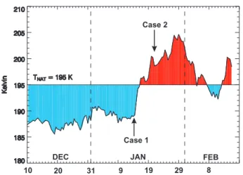
The meteorological conditions during the SOLVE2 win-ter period allow us to study the performance of NOGAPS-ALPHA prognostic ozone fields under both relatively quies-cent and disturbed polar vortex conditions. From early De-cember 2002 to mid-January 2003, the Arctic polar vortex was relatively stable and lower stratospheric temperatures were cold enough to form PSCs. A stratospheric warming beginning on or around 17 January 2003 caused the vortex to split into two distinct lobes by 21 January (Urban et al., 2004). Figure 1 depicts the rapid change in 30 hPa minimum temperatures over the Northern polar region during January 2003.

This paper presents results from NOGAPS-ALPHA hind-cast runs (with prognostic ozone activated) that span these two distinctly different periods in January 2003. Case 1 (see Fig. 1) corresponds nominally to the DC-8 flight of 14 Jan-uary 2000, during the period of cold, relatively undisturbed

DEC 9 31 20 10 19 29 JAN FEB 8 Case 1 Case 2

Fig. 1. Time series of minimum 30 hPa temperatures within 60◦– 90◦N during the period 10 December 2002–18 February 2003 taken from operational NOGAPS MVOI analyses. Dotted vertical lines separate individual months. DC-8 flights on 14 January and 21 Jan-uary are indicated as Case 1 and Case 2, respectively. Horizontal line denotes nominal 195 K PSC formation temperature threshold at 30 hPa.

vortex conditions that existed during 11–16 January. Our NOGAPS-ALPHA forecasts are initialized on 11 January and run throughout this 5-day period. Our comparisons here focus on the full ozone profile throughout the stratosphere, and thus we compare mostly with satellite data since DC-8 ozone profiles do not extend quite as high. Case 2 focuses on the DC-8 flight on 21 January, toward the end period of the rapid initial warming of the stratosphere and splitting of the vortex during 17–22 January. The complex meteorology of this event is used as a rigorous test of NOGAPS-ALPHA model dynamics and transport. For this case, we compare more closely with DC-8 lidar data along a flight track at heights ∼13–30 km. At the altitudes and latitudes of the SOLVE2 DC-8 flights, the ozone photochemical relaxation times are fairly long, and so model initialization and trans-port effects should dominate. These case studies are the first assessments of NOGAPS-ALPHA model performance.

The paper is organized as follows: Sect. 2 provides a description of the major modifications of the NOGAPS-ALPHA GCM compared to the current operational NO-GAPS; Sect. 3 gives an overview of the various data sources used to validate the NOGAPS-ALPHA simulations; Sect. 4 focuses on the period of 11–16 January 2003, present-ing an intercomparison of 3 different ozone photochemistry schemes in NOGAPS-ALPHA validated with a combina-tion of SAGE III and POAM III ozone profile measure-ments; Sect. 5 presents an assessment of NOGAPS-ALPHA prognostic ozone during the rapidly developing stratospheric warming period 17–22 January 2003; Sect. 6 summarizes these results and outlines future research directions.

2 Model description

This section presents a brief overview of the new NOGAPS-ALPHA NWP model. Additional details can be found in Eckermann et al. (2004b).

2.1 Overview of NOGAPS GCM and Operational Schemes The NOGAPS GCM is an Eulerian spectral model currently run operationally with triangular truncation at zonal and meridional wavenumber 239 (T239), roughly equivalent to 0.5◦latitude–longitude spacing. It utilizes a generalized ver-tical coordinate within an energy conserving verver-tical finite difference formulation (Kasahara, 1974; Simmons and Bur-ridge, 1981; Hogan and Rosmond, 1991). The model’s dy-namical variables are relative vorticity, divergence, virtual potential temperature, specific humidity, and terrain (surface) pressure. The model is central in time with a semi-implicit treatment of gravity wave propagation and Robert (Asselin) time filtering (Simmons et al., 1978).

The current operational model’s physics packages in-clude a bulk Richardson number-dependent vertical mixing scheme (Louis et al., 1982), a time-implicit Louis surface flux parameterization (Louis, 1979), orographic gravity wave and flow-blocking drag (Webster et al., 2003), shallow cu-mulus mixing of moisture, temperature, and winds (Tiedtke, 1984), the Emanuel cumulus parameterization (Emanuel and Zivkovic-Rothman, 1999; Peng et al., 2004), convec-tive, stratiform and boundary-layer cloud parameterizations (Slingo, 1987; Teixeira and Hogan, 2002), and a shortwave and longwave radiation scheme (Harshvardhan et al., 1987). These operational schemes are available for use in NOGAPS-ALPHA and can be activated or deactivated as part of the model development process. The following sec-tions describe new features in NOGAPS-ALPHA which are not, at present, part of the operational NWP model.

2.2 Vertical Coordinate

Designed primarily for tropospheric applications, the oper-ational NOGAPS model currently uses a terrain-following

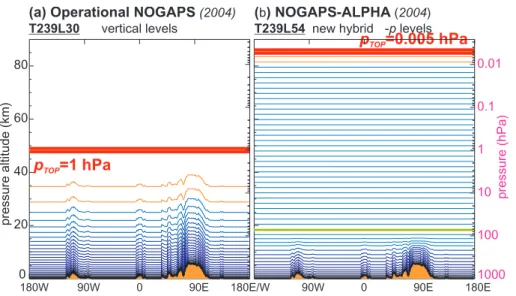
σ coordinate with 30 vertical levels (L30) extending from the surface to 1 hPa (∼48 km altitude), as shown in Fig. 2a. Thermal and mechanical damping and enhanced horizontal spectral diffusion are applied to the top 2 full model layers to form a sponge layer (see orange half levels in Fig. 2a), which means that undamped operational output extends up to only the third full model level at ∼22 hPa.

To improve middle atmosphere simulations (Simmons and Burridge, 1981; Trenberth and Stepaniak, 2002), NOGAPS-ALPHA replaces the σ coordinate with a hybrid σ -p ver-tical coordinate that transitions from terrain-following near the surface to pure pressure levels at ∼72.6 hPa (Ecker-mann et al., 2004b). Figure 2b demonstrates how this co-ordinate smoothly transitions model layer pressure height

180W 90W 0 90E 0 20 40 60 80 pressure altitude (km) pTOP=1 hPa

(a) Operational NOGAPS

vertical levels (2004) T239L30 s 180E/W pTOP=0.005 hPa 1000 100 10 1 0.1 0.01 pressure (hPa) 90W 0 90E 180E ( ) NOGAPS-ALPHAb ( )

new hybrid - levelsp2004

T239L54 s

Fig. 2. Vertical levels around 34.5◦N for: (a) operational NOGAPS 30 level (L30) model, with pt op=1 hPa; (b) new NOGAPS-ALPHA 54

level (L54) model with pt op=0.005 hPa, using new hybrid σ -p formulation with a first purely isobaric level at 72.6 hPa, shown in yellow.

Top 3 model half levels (marked in orange) span the top 2 full model layers in NOGAPS where enhanced damping and diffusion act as a sponge layer.

thicknesses to constant thicknesses of ∼2 km in the strato-sphere over arbitrary topography for our current 54 level NOGAPS-ALPHA formulation. This uniform vertical reso-lution throughout the middle atmosphere is similar to the cur-rent ECMWF model configuration and offers the prospect of better resolved middle atmosphere dynamics and transport. 2.3 Radiation

Raising the top boundary of the NOGAPS-ALPHA model requires an improved treatment of middle atmospheric ra-diative heating. To this end, we have replaced the opera-tional model’s current radiative heating scheme (Harshvard-han et al., 1987) with the CLIRAD longwave (Chou et al., 2001) and shortwave (Chou and Suarez, 2002) schemes, im-proving the net heating calculations at all levels but partic-ularly in the middle atmosphere. Specifically, the updated CLIRAD shortwave heating rates include contributions from O2 and near-infrared CO2 bands that are not contained in the operational radiative heating scheme and led to underes-timated peak shortwave heating in the middle atmosphere of as much as 1–2 K day−1_{(Eckermann et al., 2004b).}

Shortwave heating and longwave cooling rates are cur-rently computed using seasonally-varying two-dimensional (height-latitude) climatological ozone and water vapor mix-ing ratios. For NOGAPS-ALPHA, these values have been updated and extended vertically using the monthly mean ozone climatology of Fortuin and Kelder (1998) (1000– 0.3 hPa) and Halogen Occultation Experiment (HALOE) wa-ter vapor measurements from 100–0.3 hPa (Pumphrey et al., 1998). Above the 0.3 hPa level, the ozone and water va-por mixing ratios are based on long-term climate output from NRL’s CHEM2D model (McCormack and Siskind, 2002).

2.4 Gravity Wave Drag

Operational NOGAPS lacks any parameterization of middle atmospheric gravity wave drag (GWD). It is well-known that lack of GWD leads to, among other things, a cold bias in predicted wintertime Arctic stratospheric temperatures. As a result, operational NOGAPS temperatures tended to overpre-dict geographical regions of PSC formation during SOLVE2 (this cold bias should be borne in mind when interpreting Fig. 1). The extension of NOGAPS-ALPHA into the meso-sphere should allow it to better simulate vertically deep dia-batic descent through the vortex which can alleviate this cold bias, given sufficient resolution and good parameterizations of middle atmospheric GWD (Austin et al., 2003).

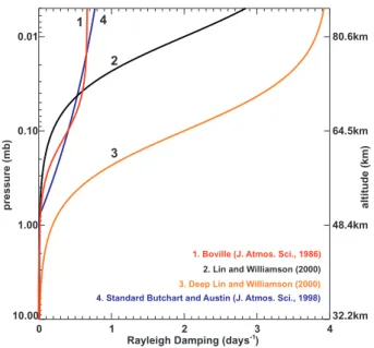
To this end, we have coded and implemented within NOGAPS-ALPHA four GWD schemes. These four schemes consist of two spectral GWD schemes for the middle atmo-sphere (Hines, 1997; Alexander and Dunkerton, 1999), a new orographic GWD scheme (Kim and Doyle, 20041) based to some extent on the work of Kim and Arakawa (1995), and a GWD parameterization scheme for convectively generated gravity waves based on Chun and Baik (2002). The perfor-mance of these schemes in NOGAPS-ALPHA forecast runs has not yet been rigorously tested. Therefore, the model cal-culations presented here utilize two different Rayleigh fric-tion (RF) profiles applied to the zonal winds above ∼40 km (see Fig. 3). The first RF profile we used is a modification of a standard profile proposed by Lin and Williamson (2000) for dynamical core tests: their original profile and our mod-1_{Kim, Y.-J. and J.D. Doyle: Offline evaluation of an orographic}

gravity wave drag scheme extended to include the effects of oro-graphic anisotropy and flow blocking, Q. J. R. Meteorol. Soc., sub-mitted, 2004.

ified “deep” version are shown in Fig. 3 as profiles 2 and 3, respectively. This modified profile imposes very strong drag on the zonal winds in the upper stratosphere and mesosphere. The second profile we use (profile 4 in Fig. 3) is based on the “standard” RF profile used by Butchart and Austin (1998) in the UKMO Unified Model. It imposes less drag on the zonal winds, and is more representative of various pro-files used in many global models that are also available for use in NOGAPS-ALPHA (Boville, 1986; Eckermann et al., 2004b). All NOGAPS-ALPHA simulations presented here used the Butchart and Austin (1998) RF profile. In addition, orographic GWD, specified using the Palmer et al. (1986) scheme, was applied from the surface up to 150 hPa. This is done to keep the orographic GWD scheme in NOGAPS-ALPHA consistent with the NOGAPS configuration that was operational during the SOLVE2 period.

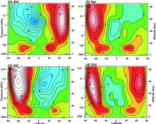
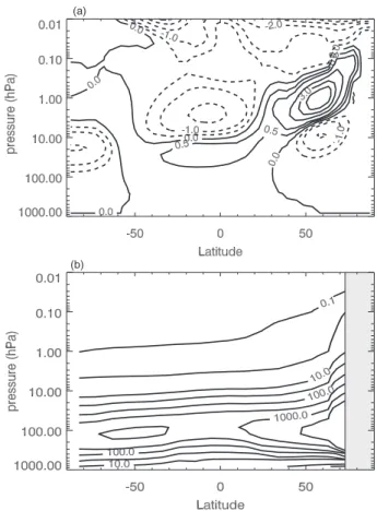
Although the use of Rayleigh friction is a crude proxy for mesospheric GWD that can reduce realistic middle at-mospheric variability (e.g. Shepherd et al., 1996; Lawrence, 1997), it’s performance has been documented in previous global NWP and climate models (see, e.g., Shepherd et al., 1996; Butchart and Austin, 1998; Pawson et al., 1998). We have tested mesospheric Rayleigh friction in a 5-year free-running simulation of an earlier low horizontal resolution T79L54 version of NOGAPS-ALPHA using the Rayleigh friction profile of Boville (1986) (profile 1 in Fig. 3). Fig-ure 4 plots monthly averaged zonal-mean zonal winds for January, April, July, and October, which show reasonable agreement with climatological values (Randel et al., 2004). Figure 5 plots the mean meridional circulation computed as a mass flux from the residual mean mass stream function for January, April, July, and October. We see that, despite be-ing designed primarily for short-term NWP, the NOGAPS-ALPHA middle atmosphere reproduces a realistic climato-logical Brewer-Dobson stratospheric circulation and a clear pole-to-pole mesospheric residual circulation.

2.5 Upper Level Initialization

NOGAPS-ALPHA is initialized here by combining archived operational output from FNMOC’s Multivariate Optimum Interpolation (MVOI) system (up to 10 hPa) (Goerss and Phoebus, 1992) with an experimental “STRATOI” product (based on TOVS radiances) from 10–0.4 hPa. Above 0.4 hPa, NOGAPS-ALPHA extrapolates the topmost initializa-tion wind and temperature fields by progressively relax-ing them with increasrelax-ing altitude to climatological values from the 1986 COSPAR International Reference Atmosphere (CIRA) (Fleming et al., 1990). Given the unreliability of mesospheric CIRA winds during certain months, particularly near the equator (Randel et al., 2004), we have created an ad-ditional option of relaxing to climatological wind fields from the Upper Atmosphere Research Satellite (UARS) Reference Atmosphere Project (URAP) (Swinbank and Ortland, 2003). Final extrapolated temperature profiles are then used to

spec-0 1 2 3 4

Rayleigh Damping (days-1₎

10.00 1.00 0.10 0.01 pressure (mb) 32.2km 48.4km 64.5km 80.6km altitude (km)

4. Standard Butchart and Austin (J. Atmos. Sci., 1998)

3. Deep Lin and Williamson (2000)

2. Lin and Williamson (2000) 1. Boville (J. Atmos. Sci., 1986) 1

2

3 4

Fig. 3. Rayleigh friction profiles used in NOGAPS-ALPHA.

ify geopotential profiles using hydrostatic integration. For further details, see Eckermann et al. (2004b).

In late 2003, initialization of the operational NOGAPS model transitioned from MVOI to the NRL Variational Data Assimilation System (NAVDAS), which currently provides fields up to ∼4 hPa (Daley and Barker, 2001; Goerss et al., 2003). NAVDAS began direct assimilation of AMSU-A ra-diance measurements in June 2004, providing additional mo-tivation for development of a prognostic ozone scheme in NOGAPS-ALPHA.

2.6 Prognostic Ozone

A new three-dimensional (3D) prognostic ozone capability has been implemented in NOGAPS-ALPHA. Since FNMOC does not at present assimilate ozone, here for NOGAPS-ALPHA we use assimilated ozone fields from two different systems. The first is 2◦×2.5◦ (latitude/longitude) analyzed 3D ozone mixing ratios from the GEOS data assimilation system, issued by NASA’s Global Modeling and Assimila-tion Office (GMAO) (Stajner et al., 2001). The second is archived ozone initialization fields from the ECMWF IFS. Both assimilated ozone fields were interpolated to 1◦_×1◦

pressure-level fields for use in NOGAPS-ALPHA as an ini-tialization field for ozone.

Two distinct prognostic ozone variables can be activated in NOGAPS-ALPHA. The first constituent represents “pas-sive” ozone, where initialized ozone is subsequently sub-jected only to advection by the model’s forecast meteorology. The second constituent, so–called “active” ozone, is subject to both advection and parameterized photochemical produc-tion and loss. The passive ozone tracer is a powerful tool for diagnosing model transport in the middle atmosphere.

Pressure (hPa)

(a) Jan (b) Apr

Altitude (km) (c) Jul (d) Oct -50 -30 -30 -10 -10 -10 10 10 10 10 10 30 30 30 50 50 70 70 90 1000 100 10 1 0.1 0.01 0 20 40 60 80 -90 -60 -30 0 30 60 90 -1 0 -10 -10 1 0 10 10 1 0 10 3 0 30 50 50 70 1000 100 10 1 0.1 0.01 0 20 40 60 80 -90 -60 -30 0 30 60 90 -50 -3 0 -3 0 -1 0 -10 -1 0 10 10 10 10 3 0 30 30 5 0 50 7 0 70 9 0 90 110 130 1000 100 10 1 0.1 0.01 Pressure (hPa) 0 20 40 60 80 -90 -60 -30 0 30 60 90 Latitude 1000 0.01 -1 0 -10 -10 10 1₀ 1₀ 10 10 10 1 0 30 3₀ 3 0 30 30 50 50 50 70 90 100 10 1 0.1 0 20 40 60 80 -90 -60 -30 0 30 60 90 Latitude Altitude (km)

Fig. 4. Monthly zonal mean zonal winds from a 5-year T79L54 NOGAPS-ALPHA simulation for January, April, July, and October. Contours

are drawn every 10 ms−1. Westerly winds are shaded yellow to red, easterly winds are shaded green to blue.

-1.0·10 0 -1.0·10 -1 -2.0·10 -2 -1.0·10 -2 -2.0·10 -3 -2.0·10 -3 -1.0·10 -3 -1.0·10 -3 0 0 0 0 0 1.0·10 -3 2.0·10 -3 1.0·10 -2 2.0·10 -2 1.0·10 -1 2.0·100 1000 100 10 1 0.1 0.01 0 20 40 60 80 Altitude (Km) -90 -60 -30 0 30 60 90 -2.0·10-1.0·1000 0 0 0 0 0 0 0 1.0·10 -3 2.0·10-3 1.0·10 -2 2.0·10 -2 2.0·10 -1 1.0·10 0 2.0·100 1000 100 10 1 0.1 0.01 0 20 40 60 80 Altitude (Km) -90 -60 -30 0 30 60 90 Latitude -1.0·10 -1 -2.0·10 -2-1.0·10-2 -1.0·10 -3 0 0 0 0 1.0·10-3 1.0·10 -3 1.0·10 -3 2.0·10 -3 2.0·10 -3 1.0·10-2 2.0·10-2 1.0·10 -1 1.0·10 0 2.0·100 1000 100 10 1 0.1 0.01 Pressure (hPa) 0 20 40 60 80 -90 -60 -30 0 30 60 90

(a) Jan (b) Apr

-1.0·101 -2.0·10-1.0·100 0 -1.0·10 -1 -2.0·10 -2 -1.0·10 -2 -2.0·10 -3 -2.0·10 -3 -1.0·10 -3 -1.0·10 -3 0 0 0 0 0 1000 100 10 1 0.1 0.01 Pressure (hPa) 0 20 40 60 80 -90 -60 -30 0 30 60 90 Latitude (c) Jul (d) Oct

Fig. 5. Monthly mean meridional mass stream function from a 5-year T79L54 NOGAPS-ALPHA simulation for January, April, July, and

October. Distance between contour lines is proportional to strength of mass flux. Clockwise circulation (positive contours) is shaded yellow to red, counter-clockwise circulation (negative contours) is shaded green to blue. Contour values are in units of 1010kg s−1.

By taking the difference between active and passive ozone fields, one can distinguish between dynamical and photo-chemical variations in the model’s three-dimensional global ozone fields.

These ozone fields are transported globally within NOGAPS-ALPHA using the same spectral advection algo-rithms used to advect meteorological variables such as vortic-ity and specific humidvortic-ity. Over time, the spectral advection produces fine scale spectral noise in ozone mixing ratio fields (Rasch et al., 1990; Fairlie et al., 1994), which we effectively suppress by applying after each time step a small amount of

∇4horizontal spectral diffusion, with a diffusion coefficient equal to that applied to the NOGAPS-ALPHA divergence fields. For the prognostic ozone fields reported here, spec-tral diffusion was applied to the isobaric stratospheric layers only.

Since NOGAPS-ALPHA is designed to be a forecast model, calculating the ozone production and loss terms us-ing a complete photochemical model is too computationally expensive at present. Instead, the net ozone photochemical production/loss rates, (P −L), can be parameterized as fol-lows. First, we approximate net production/loss to be a func-tion of three variables: the current local ozone mixing ratio (r), local temperature (T ), and the overlying ozone column abundance (6) (Cariolle and D´equ´e, 1986; McLinden et al., 2000). By approximating this functional dependence using a truncated (linearized) Taylor Series expansion, the ozone photochemical tendency equation can then be expressed as follows: dr dt =(P − L)o+ ∂(P − L) ∂r    _o [r − ro] (1) + ∂(P − L) ∂T     o [T − To] + ∂(P − L) ∂6     o [6 − 6o] ,

where d/dt is the advective time derivative, so that when the right hand side of (1) is zero, we reproduce passive ozone. The photochemical coefficients (P − L)o, ∂(P −L)_∂r |o,

∂(P −L) ∂T |o, and

∂(P −L)

∂6 |o represent diurnally-averaged

quan-tities computed at a reference state (ro,To,6o) which is

ide-ally the photochemical equilibrium state, but when imple-mented as a model parameterization is usually in practice a 2D observed climatological state for each variable (McLin-den et al., 2000; Dethof and Holm, 2002). These photochem-ical coefficients are computed offline using a 2D (altitude-latitude) photochemical model with complete descriptions of radiation and constituent photochemistry. The partial deriva-tive terms are estimated by varying the one variable while keeping the other two reference variables constant and then estimating the derivative by linear fits to the change in pro-duction/loss (McLinden et al., 2000). Their values are tab-ulated as functions of altitude and latitude for each month of the year. Currently NOGAPS-ALPHA applies the ozone photochemistry schemes up to ∼1 hPa, then smoothly

re-(b) (a)

Fig. 6. Values of (a) the residual net ozone mixing ratio tendency

(P −L)oin ppmv month−1, and (b) photochemical relaxation time

τO3 (in days) computed for mid-January conditions with the NRL

CHEM2D model. Shaded region in (b) indicates polar night.

laxes the active ozone fields to 2D climatological mixing ra-tios in the mesosphere.

Section 4 compares results from three different lin-earized photochemistry parameterizations in order to de-termine the sensitivity of the prognostic ozone simulations to the details of the parameterization coefficients. Specifi-cally, we compare NOGAPS-ALPHA “active” ozone fields computed using the Cariolle and D´equ´e (1986) coefficients (hereafter CD86), the McLinden et al. (2000) “LINOZ” coefficients (hereafter LINOZ), and coefficients from the NRL CHEM2D model (hereafter CHEM2D). Note that the CHEM2D scheme currently employs only the first two terms on the right hand side of (1), representing the residual net production/loss (P −L)o and the sensitivity to changes in

local ozone mixing ratio, ∂(P −L)_∂r |_o, respectively. The lat-ter lat-term is often expressed in lat-terms of the photochemical relaxation time for ozone, τO3=−[

∂(P −L)

∂r |o]

−1_{. Figure 6} plots (P −L)o and τO3 calculated with the NRL CHEM2D

model for mid-January conditions. The very small resid-ual tendency (P −L)oand very long relaxation times τO3 at

high Northern winter latitudes indicate that transport effects should generally dominate over photochemistry during the

SOLVE2 campaign. However, the ozone simulations in Sec-tion 4 demonstrate that stratospheric ozone forecast skill in this region can be sensitive to the treatments of both photo-chemistry and transport.

3 Data description

As a first test of the new NOGAPS-ALPHA model per-formance, we compare simulations of stratospheric ozone and temperature for select periods during the SOLVE2 cam-paign with observations from a variety of sources. These sources include operational ECMWF meteorological analy-ses, satellite-based measurements of the total ozone column abundance and ozone profiles, and data records from instru-ments aboard the NASA DC-8 aircraft. A short description of each data source follows.

3.1 Meteorological analyses

During the SOLVE2 period, operational NOGAPS analyses from the MVOI system (Goerss and Phoebus, 1992) were issued at 0, 6, 12, and 18 Z. These gridded (1◦×1◦ lati-tude/longitude) fields include horizontal winds, temperature, geopotential height, dew point depression, vorticity, and di-vergence on a fixed set of pressure levels extending up to 10 hPa. In addition, 6-hourly high-resolution (T511L60) op-erational analyses from the ECMWF IFS provided winds, temperature, geopotential height, vorticity, divergence, and ozone mass mixing ratio (ECMWF, 1995). The ECMWF fields are issued on native model levels (see, e.g. Dethof, 2003) and a reduced (N256) Gaussian grid. For both the 14 January and 21 January case studies in the present work, (Cases 1 and 2 respectively) operational T239L30 NOGAPS and T511L60 ECMWF meteorological analyses are used to help assess the performance of the new NOGAPS-ALPHA model.

NOGAPS-ALPHA ozone simulations use 3D strato-spheric ozone analyses output from either the NASA GEOS4 data assimilation system or the ECMWF IFS to initialize both the active and passive ozone fields (see Sect. 2.6).

Daily global GEOS4 ozone analyses at 0 Z were issued throughout the SOLVE2 winter at fixed pressure levels from 1000 hPa to 0.2 hPa with a 2◦×2.5◦latitude/longitude reso-lution. The GEOS4 system assimilates stratospheric ozone profiles and total ozone column measurements from the NOAA-16 SBUV/2 instrument. Ozone photochemical pro-duction and loss rates are specified as functions of latitude, pressure, and month (Fleming et al., 2001), with adjustments to the upper stratospheric values as in Stajner et al. (2004).

The operational ECMWF ozone assimilation (Dethof, 2003) product is based on NOAA-16 SBUV/2 profile and ERS-2 GOME total ozone measurements and uses the lin-earized ozone photochemistry scheme of Cariolle and D´equ´e (1986).

3.2 Satellite ozone measurements

The present study compares NOGAPS-ALPHA prognostic ozone simulations with measurements of the integrated col-umn ozone abundance from the Total Ozone Mapping Spec-trometer (TOMS) aboard the NASA Earth Probe satellite (McPeters et al., 1998), hereafter referred to as EPTOMS. Since the largest contribution to the total ozone column orig-inates in the lower stratosphere, where the ozone photochem-istry is slow compared to transport, this quantity provides a good test of the model’s spectral transport.

Observations of the vertical distribution of ozone come from the NASA Stratospheric Aerosol and Gas Experiment (SAGE) III instrument aboard the METEOR-3M satellite (Thomason and Taha, 2003), and from the NRL Polar Ozone and Aerosol Monitoring (POAM) III instrument aboard the CNES SPOT-4 satellite (Bevilacqua et al., 2002). Both satel-lites operate in sun-synchronous orbits that offer good cover-age of polar latitudes during winter. For the 11–22 January 2003 period, SAGE III provided 13 to 14 profiles each day over latitudes ranging from 67◦N–69◦N. The present study uses the Version 3.04 “least squares” SAGE III retrievals be-tween 200–1 hPa. For the same time period, POAM III pro-vided 14 to 15 stratospheric profiles (Version 3) each day from 250–0.1 hPa over the 64◦N–65◦N latitude range. The combined random and systematic errors in the stratospheric ozone profiles are <5% for both instruments. Both SAGE III and POAM III retrievals provide profiles of ozone molecular concentration that are converted to volume mixing ratio us-ing temperature and pressure analyses. SAGE III retrievals use temperature and pressure information from the National Centers for Environmental Prediction (NCEP) up to 1 hPa. POAM III retrievals use temperature and pressure informa-tion provided by the United Kingdom Meteorological Of-fice (UKMO). Section 4 compares NOGAPS-ALPHA ozone hindcasts for 11–16 January 2003 (Case 1) with EPTOMS, SAGE III, and POAM III observations as well as ECMWF operational ozone analyses and forecasts.

3.3 DC-8 measurements

Of the 14 different experiments on the NASA DC-8 air-craft payload for SOLVE2, two are particularly well-suited for comparison with NOGAPS-ALPHA simulations. The first experiment is the NASA Langley Differential Absorp-tion Lidar (DIAL). DIAL measures backscattered radiaAbsorp-tion near wavelengths of 301 nm and 311 nm, providing (among other things) in-flight ozone profiles with a vertical resolu-tion of 750 m over the altitude region from ∼1 km above the aircraft up to 22–26 km under ideal conditions (Grant et al., 2003). The second experiment is the NASA Goddard Air-borne Raman Ozone Temperature and Aerosol Lidar (ARO-TAL). AROTAL uses a combination of Rayleigh and Ra-man backscattered radiation at 355 nm to retrieve tempera-ture profiles up to 60 km with a vertical resolution of 0.5–

1.5 km (Burris et al., 2002). This instrument also utilizes a differential absorption technique to obtain ozone profiles up to ∼30 km, even in the presence of aerosols and clouds. Sec-tion 5 presents a combinaSec-tion of both DIAL and AROTAL ozone profiles as a means of validating high resolution T239 NOGAPS-ALPHA prognostic ozone simulations along indi-vidual DC-8 flight tracks during the 21 January 2003 strato-spheric warming case (i.e. Case 2).

4 Case 1: 11–16 January 2003

4.1 Description

As Fig. 1 shows, 30 hPa temperatures over the polar region were cold enough for PSCs to form during the early winter of 2002–2003. The DC-8 flight on 14 January 2003 was the last to take place before the stratospheric warming event in mid-January (see Fig. 1 and Sect. 5). During the 14 January flight, instruments aboard the DC-8 detected a small region of PSCs over the southern tip of Scandinavia.

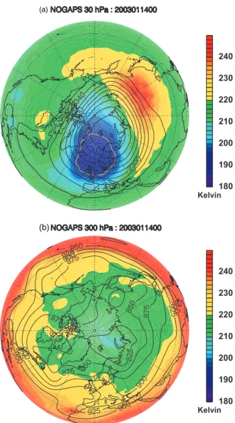
Figure 7a plots NOGAPS MVOI analyses of 30 hPa tem-peratures and geopotential heights on 14 January 2003 at 0 Z. The region where PSCs were detected lies within a larger synoptic-scale area of cold temperatures. Figure 7b plots the corresponding temperatures and heights at 300 hPa, show-ing a pronounced anti-cyclonic feature over Western Europe. This type of feature produces a combination of upward verti-cal motion and quasi-isentropic horizontal transport in the lowermost stratosphere, leading to a divergence of ozone-rich air out of the column (see, e.g. Rood et al., 1992; Or-solini et al., 1995). These localized, reversible occurrences of low total ozone, often referred to as extreme ozone minima or ozone “mini-holes”, are common occurrences with the pas-sage of an intense upper tropospheric anticyclone (Newman et al., 1988; McCormack and Hood, 1997; James, 1998). In certain cases, the resulting adiabatic cooling in the lower stratosphere can be sufficiently strong to produce tempera-tures below 195 K, which is a typical threshold temperature for the formation of nitric acid trihydrate (NAT) particles that constitute Type I PSCs (Teitelbaum et al., 2001; WMO, 2003).

Figure 8 plots total ozone column measurements from the NASA EPTOMS instrument on 14 January 2003. The heavy red contour highlights the total ozone minimum near 10◦W– 30◦_{E where total ozone values fall below 235 Dobson units}

(DU). This region coincides with the minimum in 30 hPa temperatures and maximum in 300 hPa geopotential heights shown in Fig. 7. Conditions on 14 January 2003 provide a good first test of the ability of NOGAPS-ALPHA to simu-late this interaction between tropospheric and stratospheric dynamics and its impact on the ozone distribution.

To determine the sensitivity of the model ozone simu-lations to the linearized photochemistry parameterization, we conducted a series of low-resolution T79 (∼1.5◦

lati-(b) (a) 180 190 200 210 220 230 240 Kelvin 180 190 200 210 220 230 240 Kelvin

Fig. 7. Operational 1◦×1◦NOGAPS MVOI analyses of geopo-tential height in dam (solid contours) and temperature in Kelvin (colors) on 14 January 2003 at 0 Z for (a) 30 hPa and (b) 300 hPa. 30 hPa temperatures below 195 K are enclosed with a yellow con-tour. Polar projection extends to 20◦N.

tude/longitude spacing) simulations using three different sets of linearized photochemistry coefficients. These include the most recent version of the CD86 scheme, currently used in the ECMWF IFS (H. Teyssedre, personal communication), the LINOZ scheme, and the NRL CHEM2D scheme (see Sect. 2.6 for details). Our goal is to determine which scheme most closely reproduces the observed 3D ozone distribution poleward of 20◦N over the period 11–16 January 2003. 4.2 Comparison with ozone analyses

For each simulation, both active and passive ozone fields were initialized using ozone mixing ratio analyses from the

Fig. 8. EPTOMS total ozone on 14 January 2003. Polar

projec-tion extends to 20◦N. White areas denote missing data. Heavy red contour encloses area where total ozone column abundance is be-low 235 Dobson units (DU). Locations of POAM III (crosses) and SAGE III (circles) ozone profile measurements on this date are also indicated.

NASA GEOS4 system (Stajner et al., 2001, 2004). Figure 9a plots the initial NOGAPS-ALPHA active/passive ozone mix-ing ratios as a function of pressure and longitude at 64.9◦N on 11 January 2003 at 0 Z. At this latitude, the initial NOGAPS-ALPHA (GEOS4) ozone distribution differs sub-stantially from the ECMWF ozone analyses for the same day and same location plotted in Fig. 9b. Specifically, the ECMWF ozone mixing ratios exceed the NASA GEOS4 mixing ratios by more than 2 ppmv between 30◦W–30◦E. Figure 9c shows a series of ozone mixing ratio profiles from the POAM III instrument on 11 January 2003. The POAM III measurements confirm the presence of low ozone mix-ing ratios between 30◦W–30◦E that are not captured in the ECMWF analysis.

This discrepancy between the GEOS4 and ECMWF ozone analyses over the North Atlantic sector is common through-out the SOLVE2 period poleward of ∼60◦N; at lower lati-tudes, however, both the ECMWF and GEOS4 ozone prod-ucts are in good agreement. It has been pointed out by an anonymous referee that the ECMWF system (Dethof, 2003) only assimilates SBUV/2 and GOME satellite ozone obser-vations between 40◦S and 40◦N, whereas the NASA GEOS4 system (Stajner et al., 2001) incorporates SBUV/2 obser-vations at all available latitudes in its analysis. This fact may explain the large differences between the GEOS4 and ECMWF ozone analyses at high northern latitudes during the SOLVE2 campaign whenever the local ozone distribution ex-hibited large deviations from climatological values.

-180 -120 -60 0 60 120 180 Longitude 1000.0 100.0 10.0 1.0 0.1 hPa 0.750 1.50 2.25 3.00 3.75 4.50 5.25 6.00 6.75 ppmv Longitude (a) -180 -120 -60 0 60 120 180 Longitude 1000.0 100.0 10.0 1.0 0.1 hPa (b) -180 -120 -60 0 60 120 180 1000.0 100.0 10.0 1.0 0.1 hPa (c)

Fig. 9. (a) Ozone mixing ratios (ppmv) from the 11 January 2003

NASA GEOS4 analyses at 0 Z and 64.9◦N; (b) ozone mixing ratios from 11 January 2003 operational ECMWF analyses at 0 Z and 64.4◦N; (c) POAM III ozone mixing ratio measurements at 64.2◦N on 11 January 2003, with asterisks indicating latitude of individual POAM profiles and white areas indicating missing data.

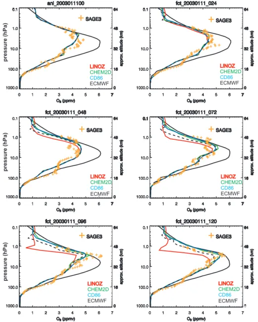
4.3 NOGAPS-ALPHA O3hindcasts: 11–16 January 2003 Figure 10 plots NOGAPS-ALPHA profiles of prognostic ozone for a 5-day simulation initialized on 11 January 2003 at 0 Z over Kiruna, Sweden (68◦N, 20◦E). This location was chosen for its proximity to both the lowest total ozone values on 14 January and the measurement latitudes of the SAGE III and POAM III instruments (see Fig. 8). Each plot compares the passive ozone (dashed black curve) with active

Fig. 10. NOGAPS-ALPHA ozone mixing ratio profiles over Kiruna, Sweden (68◦N, 20◦E) for a 5-day forecast initialized on 11 January 2003 at 0 Z using the CD86 (blue), LINOZ (red), and CHEM2D (green) photochemistry schemes. NOGAPS-ALPHA passive ozone is plotted as a dashed black curve. Co-located SAGE III profiles are plotted as orange symbols. The solid black curve denotes the corresponding ECMWF ozone analysis and forecasts initialized on 11 January 2003.

ozone computed using the CD86 coefficients (blue curve), the LINOZ coefficients (red curve), and the CHEM2D co-efficients (green curve). Also included in Fig. 10 are the ECMWF IFS ozone forecasts (solid black curve) and co-located ozone profiles from the SAGE III instrument (points) for each day. As Fig. 10 shows, the differences between the GEOS4 and ECMWF ozone initializations at this location on 11 January 2003 explain why the ECMWF ozone forecasts over the 5-day period disagree with the NOGAPS-ALPHA simulations and with the independent SAGE III measure-ments between 50–1 hPa. Interestingly, the ECMWF ozone profiles between 100–50 hPa in Fig. 10 show better agree-ment with the SAGE III observations than corresponding

NOGAPS-ALPHA ozone profiles throughout the 120-hour period. The altitude dependence of the ECMWF IFS ozone ozone forecast skill is discussed further in Section 5.

A comparison of the active ozone simulations (blue, red, and green curves in Fig. 10) shows all three photochemistry schemes exhibit little difference with the passive ozone pro-file below ∼10 hPa. In this altitude region, there is gener-ally good agreement among the three different active ozone schemes, passive ozone, and observed ozone profiles from both the SAGE III and POAM III instruments. This is to be expected since ozone photochemistry is slow compared to transport below ∼10 hPa (see Fig. 6).

Above ∼10 hPa, however, differences emerge between the active and passive ozone values, and between the individ-ual active ozone simulations as well. The differences be-tween the CD86 and CHEM2D results after 5 days are very small, and they are both in good agreement with the SAGE III measurements shown in Fig. 10. The similarity between the CHEM2D and CD86 profiles in Fig. 10 demonstrates that neglecting the temperature and column terms in Eq. (1) have a minor impact on the model ozone over 5 days at high lat-itudes in winter. In contrast, the LINOZ scheme produces excessive ozone loss that is in disagreement with the avail-able SAGE III profiles, POAM III profiles (not shown), and with the NOGAPS-ALPHA simulations using CHEM2D and CD86 photochemistry schemes.

The low upper stratospheric ozone mixing ratios in the NOGAPS-ALPHA simulation using the LINOZ scheme (red curve in Fig. 10) appear to be a consequence of unrealisti-cally large negative values in the LINOZ scheme’s (P −L)o

term. As Fig. 6 illustrates, the magnitude of the net ozone mixing ratio tendency |(P −L)o| at high northern latitudes

during January is typically small, <1 ppmv month−1, above 10 hPa and poleward of 60◦N. In comparison to both the CD86 and CHEM2D coefficients, the LINOZ |(P −L)o|term

is 5–10 times larger at all latitudes above ∼10 hPa for all months. The underlying cause for the excessive LINOZ ozone loss above 10 hPa may be related to an overestimation of the background ozone mixing ratios in the model (McLin-den et al., personal communication, 2004). Overall, the re-sults from the initial NOGAPS-ALPHA prognostic ozone simulations indicate that the LINOZ photochemistry param-eterization may not be appropriate for upper stratospheric ap-plications.

Figure 11 plots NOGAPS-ALPHA model ozone mixing ratio profiles at 65◦N and 135◦E from the same 5-day sim-ulation beginning 11 January 2003 at 0 Z. Here we com-pare results from the three different ozone photochemistry schemes, passive ozone, the ECMWF ozone forecasts, and POAM III ozone profiles. Unlike the previous case, the initial NOGAPS-ALPHA ozone mixing ratio profiles and ECMWF operational ozone analyses on 11 January over this location are in good agreement. Total ozone values on 14 January (forecast hour 96) were >475 DU over this location, and the flow at mid-stratospheric levels (see Fig. 7) brought air from lower sunlit latitudes poleward. Thus the ozone pho-tochemistry parameterization should have more of an impact on the ozone profiles at this location than for the ozone pro-files over Kiruna (see Fig. 10) where mid-stratospheric air was largely confined within polar night.

As Fig. 11 shows, the NOGAPS-ALPHA ozone simu-lations using the LINOZ scheme again produce excessive ozone loss above 10 hPa over the course of 2–3 days. How-ever, significant differences can also be seen between the results from the CD86 and CHEM2D schemes. By hour 96, both the CD86 results and the ECMWF operational ozone forecasts (which use the CD86 scheme) produce ozone

mixing ratios between 10 hPa and 50 hPa that are up to 2 ppmv less than values from either the CHEM2D or LINOZ schemes or the model passive ozone. Above 10 hPa, the LINOZ scheme again produces excessive ozone loss as com-pared to the POAM profiles. Both CHEM2D and passive ozone profiles agree well with POAM observations, espe-cially at hours 96 and 120.

For the ozone simulations over 65◦N and 135◦E shown in Fig. 11, the initial NOGAPS-ALPHA and ECMWF ozone profiles agree quite well. Over time, differences emerge between the NOGAPS-ALPHA simulations and ECMWF forecasts due to different values of the photochemical relax-ation time τO3=−[

∂(P −L)

∂r |o]

−1_{. in the lower stratosphere} (see Eq. 1). At this location, the model ozone mixing ra-tios exceed 2-D climatological values (ro) and so the ozone

tendency is negative. Typically, values of τO3 exceed 100

days in the midlatitude stratosphere near 25 km (Brasseur and Solomon, 1986). In the CD86 scheme (see, e.g. Car-iolle and D´equ´e, 1986, their Fig. 3), these values are 30–50 days. The shorter relaxation times of the CD86 scheme cause lower stratospheric ozone mixing ratios at midlatitudes to re-lax back to climatology 2–3 times faster than in either the CHEM2D or LINOZ schemes. Note that both the ECMWF and NOGAPS-ALPHA model ozone exhibit the same ten-dency toward lower ozone when the latter model employs the CD86 scheme, the same scheme currently used in the op-erational ECMWF IFS.

Next, three high resolution T239 NOGAPS-ALPHA sim-ulations were conducted over the same 5-day period starting on 11 January 2003. The T239 configuration, with an ap-proximate horizontal resolution of 0.5◦_{, matches the current}

operational NOGAPS configuration and is currently the best formulation to capture detailed structure in long-lived trac-ers. Here we compare NOGAPS-ALPHA T239 total ozone fields with total ozone fields derived from operational T511 ECMWF IFS forecasts. The largest contribution to the to-tal ozone column abundance comes from the lower strato-sphere (i.e. 10–20 km altitude), where transport effects tend to dominate over photochemistry. By using ozone photo-chemistry and initial conditions similar to the operational ECMWF model, and relaxing back to the same 2D O3 cli-matology, we can attempt to reproduce the ECMWF total ozone distribution and in doing so determine the extent to which model transport can explain the differences shown in Figs. 10 and 11.

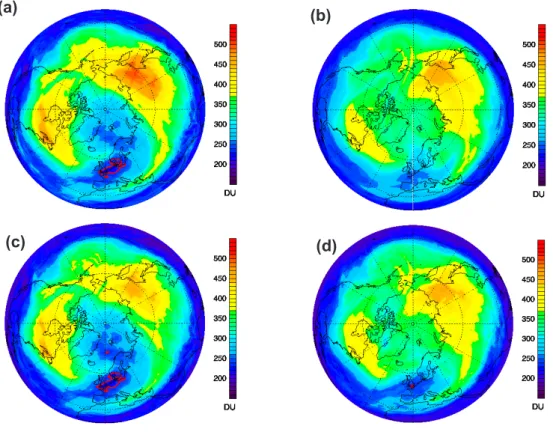
Figure 12a plots the total ozone distributions at hour 96, valid at 0 Z 14 January 2003, computed from NOGAPS-ALPHA prognostic ozone using the CHEM2D photochem-istry scheme and initialized with the NASA GEOS4 opera-tional ozone analyses. This NOGAPS-ALPHA total ozone field exhibits very good qualitative and quantitative agree-ment with the EPTOMS total ozone distribution for 14 Jan-uary (Fig. 8). Specifically, the NOGAPS-ALPHA total ozone in Fig. 12a reproduces the regions of low total ozone (<235 DU) over the North Atlantic sector, high total ozone

Fig. 11. As in Fig. 10, but now comparing NOGAPS-ALPHA ozone mixing ratio profiles at 65◦N, 135◦E with nearby POAM III ozone profiles (orange symbols).

(>475 DU) over Siberia (65◦N, 135◦E), and the “arm” of 370–420 DU values extending eastward from the Mediter-ranean that are all present in the EPTOMS observations in Fig. 8.

Figure 12b plots the corresponding 96-h operational ECMWF forecast total ozone distribution initialized on 11 January 2003 and valid for 0 Z 14 January 2003. In compar-ison with the NOGAPS-ALPHA and EPTOMS total ozone fields, the ECMWF total ozone forecast for this time exhibits much smoother zonal structure in the total ozone at middle and high latitudes. Furthermore, the ECMWF total ozone values for this date fail to fully capture the observed area

of total ozone values below 235 DU over the North Atlantic sector.

Figure 12c plots NOGAPS-ALPHA total ozone at hour 96 from a run using the CD86 photochemistry scheme and NASA GEOS4 ozone analyses for initialization. We find that the NOGAPS-ALPHA T239 run using the CD86 scheme and the GEOS4 initialization still captures the observed min-imum in total ozone over the North Atlantic sector, but over-all the zonal variations in the total ozone around 60◦N are noticeably smaller than in either the EPTOMS total ozone (Fig. 8) or the comparable NOGAPS-ALPHA T239 simu-lation using the CHEM2D photochemistry (Fig. 12a). It

(b)

(a)

(d)

(c)

Fig. 12. (a) T239L54 NOGAPS-ALPHA total ozone at hour 96 of 5-day simulation initialized 0 Z 11 January 2003 (valid 0 Z 15 January)

with NASA GEOS4 ozone analyses and using the CHEM2D photochemistry scheme; (b) total ozone from corresponding 96-h operational T511L60 96-h ECMWF IFS ozone forecast; (c) same as in (a) but using the CD86 photochemistry scheme and initialized with the NASA GEOS4 ozone analyses; (d) same as in (a) but using the CD86 photochemistry scheme and ECMWF ozone initialization. Red contours enclose regions of total ozone <235 DU.

is important to note that the only difference between the NOGAPS-ALPHA results plotted in Fig. 12a and 12c is the photochemistry scheme, indicating that differences in the de-tails of the photochemistry parameterization are affecting the total ozone distribution at high winter latitudes.

Figure 12d plots the resulting NOGAPS-ALPHA 96-h to-tal ozone forecast using the CD86 scheme and ECMWF ozone initialization. This configuration is chosen to match the ozone photochemistry and initialization used in the oper-ational ECMWF IFS forecasts. The total ozone distribution in Fig. 12d bears a very close resemblance to the operational 96-h ECMWF total ozone forecast shown in Fig. 12b. Since similar photochemistry and initialization procedures are em-ployed, the only major factor leading to differences in the NOGAPS-ALPHA total ozone in Fig. 12d and ECMWF to-tal ozone in Fig. 12b should be related to transport. The good agreement between Fig. 12b and 12d indicates that spectral transport in this 96-hour T239 NOGAPS-ALPHA hindcast compares quite well with the operational ECMWF model in the lower stratosphere for this case.

Taken together, the results in Fig. 12 demonstrate that the differences between the CD86 and CHEM2D

photochem-istry schemes can significantly impact prognostic O3 in the lower stratosphere over the course of several days. Specif-ically, the CD86 scheme tends to relax lower stratospheric ozone back to a zonal mean basic state more quickly than the CHEM2D scheme, producing total ozone fields with less zonal structure than observations indicate.

Based on these results, we find that the major differ-ences between operational ECMWF ozone forecasts and NOGAPS-ALPHA ozone simulations for the 11–16 January case are due to (1) ECMWF ozone analyses not capturing the observed ozone minimum over the North Atlantic sec-tor in the model initial conditions for 11 January 2003 (see Fig. 9); and (2) shorter stratospheric ozone photochemical re-laxation times τO3in the CD86 scheme as compared to either

the CHEM2D or LINOZ schemes. The intercomparison of different O3photochemistry parameterizations in NOGAPS-ALPHA for this case shows that the CHEM2D photochem-istry parameterization produced the best overall agreement with satellite-based ozone profile measurements and total ozone column abundances.

Fig. 13. Ertel’s potential vorticity (EPV) on the 460 K isentropic

surface computed from ECMWF T511L60 operational analysis on 21 January 2003 at 18 Z.

5 Case 2: 17–22 January 2003

5.1 Description

Case 2 corresponds to the early period of the stratospheric warming that characterized the SOLVE2 winter (Fig. 1).

Figure 13 plots values of Ertel’s potential vorticity on the 460 K isentropic surface computed from the operational T511L60 ECMWF meteorological analysis issued for 18Z on 21 January 2003. As Fig. 13 shows, the polar vortex had split into two lobes by 21 January. This disturbed strato-spheric meteorology during 17–22 January presents an ex-cellent test for the NOGAPS-ALPHA GCM generally, and its internal spectral chemical advection scheme specifically. An earlier study of prognostic skill in the lower stratosphere by Lahoz (1999) using various high-altitude versions of the United Kingdom Meteorological Office (UKMO) Unified Model focused on hindcasting during February 1994. This period yielded a minor wave-2 warming with a split vortex structure very similar morphologically to that seen in Fig. 13 (see, e.g. Lahoz’s Fig. 7a and Fig. 7b).

Lahoz (1999) noted that the UKMO models’ NWP skill tended to be poorest during this period of rapidly evolving mean flow, and cited these cases as requiring careful scrutiny when operational forecasts were used to plan aircraft flights for Arctic science missions. In light of this previous work,

-30 0 -60 -30 0 30 50 60 60 70

Kiruna

3

1-2

4

5

6

7

8

9

10

11

12

13

14

15

16

17

18

19 20

21

22

23

24

Planned Flight Path

Way Points

DC-8 SOLVE2 Science Flight

January 21, 2003

FS1

FS2

Fig. 14. Flight track of NASA DC-8 SOLVE2 science flight on

21 January 2003. Light blue curve shows planned flight track, with planned way points numbered with dark blue circles. Actual flight track, from the on-board Information Collection and Transmission System (ICATS), is plotted in dark red. This DC-8 flight ended in Lulea, southeast of Kiruna, due to icy runway conditions at Kiruna. Two flight segments chosen for further analysis are shown in light orange and light red, corresponding to flight times shown in the bottom-left of the plot.

the 17–21 January period presents a highly relevant case for studying model performance within the context of airborne SOLVE2 science flights. The rapid dynamical evolution of this case provides a rigorous test case for our new spectral advection formulation for transporting ozone. For this case, we will study prognostic ozone in the lower stratosphere only (below ∼10 hPa), where photochemical lifetimes at all lati-tudes are long compared to forecasting timescales (Fig. 6). This serves as a test of the model’s advection code using ozone as our diagnostic variable.

5.2 Lidar ozone profiles from SOLVE2 DC-8 flight To validate NOGAPS-ALPHA’s prognostic ozone during Case 2, we utilize DC-8 data acquired during a science flight on 21 January 2003 (see Fig. 14). For comparison, we have chosen two flight segments for detailed analysis. The first flight segment, denoted FS-1, is shown in light-orange in Fig. 14. From Fig. 13, we see that first part of FS-1 heads away from the split polar vortices as the aircraft flies south of Iceland from Kiruna. The second part of FS-1 then heads back into the split polar vortices as the DC-8 proceeds north toward Greenland. The second flight segment (FS-2) in-volves an approximately linear transect from southern Green-land to Svalbard, flying across the split vortex lobe structures

Ozone Mixing Ratios Along DC-8 Flight Segment 1: January 21, 2003

13.5 14.0 14.5 15.0 15.5

DC-8 Flight Time (Hours UT) 15 20 25 30 geometric altitude (km) 0.5 0.5 1 ₁ 1 2 ₂ 3 3 3 4 13.0 13.5 14.0 14.5 15.0 15.5 16.0

DC-8 Flight Time (Hours UT)

1 1 2 3 3 3 4 4 5 5 6 7 0 ppmv >_7.0

(a) DIAL Lidar (b) AROTAL Lidar

5

Fig. 15. Ozone mixing ratios (ppmv) as a function of geometric altitude along DC-8 flight segment 1 (FS-1) as measured by (a) DIAL lidar

and (b) AROTAL lidar on 21 January 2003. The AROTAL values were smoothed along the time axis using a 9-point running average to reduce noisiness at upper levels caused by acquisition of data in sunlight. Color scale is 0–7 ppmv: values >7 ppmv are shaded white for AROTAL. White regions for DIAL denote missing data.

Ozone Mixing Ratios Along DC-8 Flight Segment 2: January 21, 2003

(a) DIAL Lidar (b) AROTAL Lidar

17.5 18.0 18.5 19.0 19.5 20.0 20.5

DC-8 Flight Time (Hours UT) 15 20 25 30 geometr ica lti tu de (k m ) 1 2 2 3 3 3 3 4 0 ppmv >_7.0 17.5 18.0 18.5 19.0 19.5 20.0 20.5 21.0 1 3 3 3 3 2 4

DC-8 Flight Time (Hours UT)

Fig. 16. Ozone mixing ratios (ppmv) as a function of geometric altitude along DC-8 flight segment 2 (FS-2) as measured by (a) DIAL

lidar and (b) AROTAL lidar on 21 January 2003. AROTAL values were not smoothed here due to greater signal-to-noise provided by data acquisition in polar night. Color scale is 0–7 ppmv: values >7 ppmv are shaded white for AROTAL. White regions for DIAL denote missing data.

shown in Fig. 13. FS-2 potentially profiles mid-latitude low-PV air from a filament separating the two lobes at the ap-proximate midpoint of this flight segment.

Figures 15 and 16 plot ozone mixing ratios acquired along FS-1 and FS-2, respectively, from the DIAL and AROTAL li-dar systems on board the DC-8. Both lili-dar systems reproduce the same major features. For FS-1, the lidar data in Fig. 15 show ozone mixing ratios near 20 km decreasing slightly as the DC-8 heads southwest to Iceland, then increasing sub-stantially through the stratosphere during part of its

north-ward trek tonorth-ward the coast of Greenland. For FS-2, mix-ing ratios are generally smaller, with AROTAL upper-level mixing ratios decreasing with time along the flight segment. Near the midpoint of FS-2, both lidars show a sloping upward bulge of low ozone air at ∼15 km and a narrow increase in ozone mixing ratio at ∼19:20 Z at heights ∼15–20 km and, in AROTAL, again at ∼30 km. This seems to be a possible ozone signature of the filament of low-PV air separating the split vortex lobes, noted in Fig. 13.

(a) GMAO Ozone Analysis: 2.5 x2 : 12:00Zo o (b) ECMWF Ozone AnalysisT511L60: 18:00Z

Analyzed Ozone Mixing Ratios Along DC-8 Flight Segment 1: January 21, 2003

DC-8 Flight Time (Hours UT) 15 20 25 30 35 pressure he ig ht (k m ) 1 1 2 2 3 3 4 4 5 5 6 13.0 13.5 14.0 14.5 15.0 15.5 13.0 13.5 14.0 14.5 15.0 15.5 1 1 2 2 3 3 4 4 5 5 6 6 13.0 13.5 14.0 14.5 15.0 15.5 13.0 13.5 14.0 14.5 15.0 15.5 DC-8 Flight Time (Hours UT)

Fig. 17. Analysis ozone mixing ratios (ppmv) as a function of pressure altitude along the DC-8 flight segment 1 (FS-1) from (a) GEOS4

2.5◦×2◦analysis, and (b) operational ECMWF analysis fields from T511L60 model (on a reduced N256 grid). Both analyses are for 21 January 2003: GEOS4 is taken at 12 Z, ECMWF is taken at 18 Z. Altitude range is extended to ∼35 km to account for differences in pressure and geometric altitudes (see Fig. 19).

(a) GMAO Ozone Analysis: 2.5 x2 : 18:00Zo o

DC-8 Flight Time (Hours UT) 15 20 25 30 35 pressure height (km) 1 1 2 2 3 3 4 4 5 5 17.5 18.0 18.5 19.0 19.5 20.0 20.5 17.5 18.0 18.5 19.0 19.5 20.0 20.5 17.517.5 18.0 18.5 19.0 19.5 20.0 20.5 1 ₁ 2 2 3 ₃ 4 ₄ 5 6 18.0 18.5 19.0 19.5 20.0 20.5

(b) ECMWF Ozone Analysis:T511L60: 18:00Z

Analyzed Ozone Mixing Ratios Along DC-8 Flight Segment 2: January 21, 2003

DC-8 Flight Time (Hours UT)

Fig. 18. Analysis ozone mixing ratios (ppmv) as a function of pressure altitude along the DC-8 flight segment 2 (FS-2) from (a) GEOS4

2.5◦×2◦analysis, and (b) operational ECMWF analysis fields from T511L60 model (on a reduced N256 grid). Both analyses here are for 21 January 2003 at 18 Z. Altitude range is extended to ∼35 km to account for differences in pressure and geometric altitudes (see Fig. 19).

5.3 Comparison with ozone analyses

We begin by comparing the ECMWF and GEOS4 ozone analyses along the DC-8 flight track to determine if either system captures any of the features seen in the DC-8 li-dar data. Fig. 17 plots ozone mixing ratios for 21 January 2003 from the GEOS4 analysis (at 12 Z) and the operational ECMWF analysis (at 18 Z), these two times roughly span-ning the 13–16 Z period of FS-1. Note the much coarser

spatial resolution of the GEOS4 ozone analysis that provides initial conditions for prognostic ozone in NOGAPS-ALPHA. Both analyses capture the downward sloping ozone isopleths at ∼20–30 km. The ECMWF analysis also captures the re-duction in ozone at ∼20 km from ∼13:30–14:30 Z and the sudden increase at ∼14:30 Z.

Figure 18 plots ozone analyses along FS-2, using 18 Z fields for both analyses in this case. Both analyses cap-ture large ozone mixing ratios at upper levels at the start

(a) Ozone Versus Pressure Height

NOGAPS-ALPHA T239L54 Ozone Along Flight Segment 2: Initialized 2003011700, +114 Hour Forecast

17.5 18.0 18.5 19.0 19.5 20.0 20.5 DC-8 Flight Time (Hours UT) 15 20 25 30 35 pressure height (km) 1 ₁ 2 2 3 ₃ 4 4 4 5 17.5 18.0 18.5 19.0 19.5 20.0 20.5 17.5 18.0 18.5 19.0 19.5 20.0 20.5 geopotential height (km) 1 1 2 2 3 3 4 4 4 5 15 20 25 30 35 17.5 18.0 18.5 19.0 19.5 20.0 20.5 (b) Ozone Versus Geopotential Height

15 20 25 30 35

DC-8 Flight Time (Hours UT)

Fig. 19. NOGAPS-ALPHA T239L54 +114 h hindcast O₃(ppmv) for 21 January 2003 at 18 Z, plotted along DC-8 flight segment 2 as a function of (a) pressure height, and (b) geopotential height. The latter is more directly comparable to the geometric heights used for the lidar ozone profiles in Fig. 16; dotted pink line shows 30 km upper boundary of lidar plot.

17.5 18.0 18.5 19.0 19.5 20.0 20.5

DC-8 Flight Time (Hours UT)

15 20 25 30 35 pressure height (km) 0.51 1 2 2 3 ₃ 4 4 5 5 6 17.5 18.0 18.5 19.0 19.5 20.0 20.5 17.5 18.0 18.5 19.0 19.5 20.0 20.5 0.51 1 2 2 3 ₃ 4 ₄ 5 5 6 15 20 25 30 35 17.5 18.0 18.5 19.0 19.5 20.0 20.5

DC-8 Flight Time (Hours UT)

15 20 25 30 35 pressure height (km)

(a) ECMWF T511L60 Operational (b) NOGAPS-ALPHA T239L54

Prognostic Ozone Along Flight Segment 2: Initialized 2003011700 Using ECMWF Ozone Fields, +114 Hour Forecast

Fig. 20. (a) Archived ECMWF IFS T511L60 114-h operational forecast O₃mixing ratio (ppmv) valid for 21 January 2003 at 18 Z, plotted along DC-8 flight segment 2 as a function of pressure height; (b) corresponding 114-hour T239L54 NOGAPS-ALPHA O3hindcast initialized

with ECMWF analyzed ozone.

of the flight segment, and progressive reductions in these mixing ratios along the flight track. Near the midpoint of the flight, the higher-resolution ECMWF ozone analysis also shows what appears to be an ozone signature of the PV fila-ment separating the two vortex lobes. At ∼15 km and ∼30– 35 km, the structure is similar to that seen in the lidar data in Fig. 16. At ∼20 km, however, the lidar data show an ozone enhancement at 19:00–19:30 Z, whereas the analyzed ECMWF ozone shows a slight depletion.

5.4 NOGAPS-ALPHA O3hindcasts: 17–22 January 2003 Since NOGAPS-ALPHA is usually initialized with the coarse resolution GEOS4 ozone product shown in Figs. 17a and 18a, it is not clear whether the higher-resolution

(T239L54) NOGAPS-ALPHA model dynamics can repro-duce observed finer-scale features in the DC-8 lidar ozone profiles. This section compares T239L54 NOGAPS-ALPHA prognostic ozone fields along the selected DC-8 flight tracks on 21 January initialized with either the lower-resolution GEOS4 analyses or the higher-resolution ECMWF analyses to illustrate the impact of model initial conditions on prog-nostic O3.

Figure 19 plots T239L54 NOGAPS-ALPHA prognostic ozone fields along FS-2 for the 114-h forecast initialized us-ing GEOS4 analyzed ozone on 17 January at 0 Z (valid on 21 January 2003 at 18 Z, the approximate time of FS-2). This simulation uses the CHEM2D photochemistry scheme. The two panels plot the same data, first as a function of pressure altitude, then as a function of geopotential altitude.