HDO measurements with MIPAS

(1)

HAL Id: hal-00302504

https://hal.archives-ouvertes.fr/hal-00302504

Submitted on 19 Jan 2007

HAL is a multi-disciplinary open access

archive for the deposit and dissemination of sci-entific research documents, whether they are pub-lished or not. The documents may come from teaching and research institutions in France or abroad, or from public or private research centers.

L’archive ouverte pluridisciplinaire HAL, est destinée au dépôt et à la diffusion de documents scientifiques de niveau recherche, publiés ou non, émanant des établissements d’enseignement et de recherche français ou étrangers, des laboratoires publics ou privés.

HDO measurements with MIPAS

J. Steinwagner, M. Milz, T. von Clarmann, N. Glatthor, U. Grabowski, M.

Höpfner, G. P. Stiller, T. Röckmann

To cite this version:

J. Steinwagner, M. Milz, T. von Clarmann, N. Glatthor, U. Grabowski, et al.. HDO measurements with MIPAS. Atmospheric Chemistry and Physics Discussions, European Geosciences Union, 2007, 7 (1), pp.931-970. �hal-00302504�

(2)

ACPD

7, 931–970, 2007 HDO measurements with MIPAS J. Steinwagner et al. Title Page Abstract Introduction Conclusions References Tables Figures ◭ ◮ ◭ ◮ Back Close

Full Screen / Esc

Printer-friendly Version Interactive Discussion

EGU Atmos. Chem. Phys. Discuss., 7, 931–970, 2007

www.atmos-chem-phys-discuss.net/7/931/2007/ © Author(s) 2007. This work is licensed

under a Creative Commons License.

Atmospheric Chemistry and Physics Discussions

HDO measurements with MIPAS

J. Steinwagner1,3, M. Milz1, T. von Clarmann1, N. Glatthor1, U. Grabowski1, M. H ¨opfner1, G. P. Stiller1, and T. R ¨ockmann2,3

1

Institute for Meteorology and Climate Research, Research Center Karlsruhe, Germany

2

Institute for Marine and Atmospheric Research Utrecht, The Netherlands

3

Max Planck Institute for Nuclear Physics, Heidelberg, Germany

Received: 8 December 2006 – Accepted: 9 January 2007 – Published: 19 January 2007 Correspondence to: J. Steinwagner (joerg@steinwagner.de)

(3)

ACPD

Full Screen / Esc

EGU

Abstract

We have used high spectral resolution spectroscopic measurements from the MIPAS instrument on the Envisat satellite to simultaneously retrieve vertical profiles of H2O

and HDO in the stratosphere and uppermost troposphere. A thorough error analysis of the retrievals confirms that reliable δD data can be obtained up to an altitude of

5

45 km. Averaging over multiple orbits and thus over longitudes further reduces the random part of the error. The absolute total error of averagedδD is between 36 ‰ and

111 ‰. With values lower than 42 ‰ the total random error is significantly smaller than the natural variability ofδD. The data compare well with previous investigations. The

MIPAS measurements now provide a unique global data set of high-quality δD data

10

that will provide novel insight into the stratospheric water cycle.

1 Introduction

Water is the most important trace species in Earth’s atmosphere and heavily influences the radiative balance of the planet. In the stratosphere, it is the main substrate from which polar stratospheric clouds are formed and thus a key contributor to polar ozone

15

hole chemistry. Therefore, a possible significant increase in stratospheric water vapor as inferred from a combination of several observational series in the past is of concern (Rosenlof et al.,2001). However, the processes that control the input of water into the stratosphere are still under debate, and even the reliability of the reported water trend has been questioned (F ¨uglistaler and Haynes,2005).

20

Isotope measurements may have the potential to distinguish between different path-ways of dehydration, in particular the ”gradual dehydration” mechanism (Holton and Gettelmann,2001) and the ”convective overshooting” theory (Sherwood and Dessler, 2000). In addition, ice lofting has been recognized as an important process which causes water vapor in the lower stratosphere to be less depleted in the heavy isotopes

25

than expected from a pure gas phase distillation process, where the heavy isotopo-932

(4)

ACPD

Full Screen / Esc

EGU logues are removed preferentially in a one-step condensation process (Moyer et al.,

1996;Smith et al.,2006;Dessler and Sherwood,2003). At least on small spatial scales these processes could be clearly distinguished by their isotope signatures in recent in situ measurements in the tropical tropopause region (Webster and Heymsfield,2003). In the stratosphere, oxidation of methane produces water that is significantly enriched

5

relative to the water imported from the troposphere and thus leads to a gradual isotope enrichment (Moyer et al.,1996;Johnson et al.,2001a;Zahn et al.,2006).

As water isotope data can provide important new insight into many of the large scale transport processes in the UT/LS region a global set of high accuracy data would be particularly valuable. In previous studies of water isotopes in the UT/LS (upper

tropo-10

sphere/lower stratosphere) region space borne (e.g. ATMOS (Rinsland et al.,1991; Irion et al., 1996), sub-millimeter receiver SMR (Lautie et al., 2003)), balloon borne (e.g. mid-infrared limb sounding spectrometer MIPAS-B (Fischer, 1993; Stowasser et al., 1999), far infrared spectrometer FIRS-2 (Johnson et al., 2001a,b)), air-borne instruments (Webster and Heymsfield,2003; Coffey et al., 2006) and sampling

tech-15

niques (Pollock et al., 1980; Zahn et al., 1998; Zahn, 2001; Franz and R ¨ockmann, 2005) have been used. The results obtained in these studies provide a solid basis for advanced analysis. However, most of these measurements do not provide long term global data sets of isotopologues and thus do not allow to study seasonal effects. Fur-ther, some of the (space borne) measurements do not penetrate the atmosphere deep

20

enough to study processes at the tropopause and on the other side air borne measure-ments often do not reach far into the stratosphere. A continuous, global observation of the stratosphere and uppermost troposphere carried out by an instrument with high spectral resolution can provide a wealth of new information. In this paper we prove the feasibility of global space-borne HDO measurements with the Michelson Interferometer

25

(5)

ACPD

Full Screen / Esc

EGU

2 MIPAS

Space borne limb sounding instruments yield a sufficiently high vertical resolution to retrieve atmospheric profiles of trace species. Possibly the best suited instrument at present for stratospheric isotope research from space is MIPAS. MIPAS is a Fourier transform interferometer with a spectral resolution of 0.05 cm−1_{(apodized; 0.035 cm}−1

5

unapodized) designed to study the chemistry of the middle atmosphere detecting trace gases in the mid-infrared (4–15µm). It is flown on Envisat (Environmental Satellite)

on a sun-synchronous orbit (98◦ _{inclination, 101 min orbit period, 800 km orbit height).}

MIPAS scans the Earth limb in backward-looking viewing geometry. A complete vertical scan from the top to the bottom of the atmosphere is made up of up to 17 spectral

10

measurements (“sweeps”). The vertical step width between the sweeps is 3 km at lower heights and increases in the upper stratosphere.

3 Retrieval of HDO and H₂O

3.1 Theory

The processing software used to retrieve vertical HDO and H2O profiles from spectral

15

measurements has been described byvon Clarmann et al.(2003), where a constrained non-linear least squares approach is used. All variables related to one limb scan are fitted simultaneously as suggested by Carlotti (1988). By using Tikhonov-type regu-larization (Tikhonov,1963) smoothness of the profiles is the applied constraint. The radiative transfer through the atmosphere is modeled by the Karlsruhe Optimized and

20

Precise Radiative Transfer Algorithm, KOPRA (Stiller, 2000). Spectroscopic data is taken from a special compilation of the HITRAN 2000 data base (Rothman et al.,2003) including a number of recent updates (Flaud et al.,2003). We use the microwindow approach to select relevant spectral regions for our observations. The definition of mi-crowindows is done following an algorithm described by von Clarmann et al.(2003).

25

(6)

ACPD

Full Screen / Esc

EGU This leads to the set of microwindows we use, shown in Table1. An altitude dependent

microwindow selection was performed using a procedure suggested by Echle et al. (2000). A final optimization was done by visual inspection of resulting modeled spectra with respect to cross influences of different species.

The scientific use of the isotope data lies in the comparison of changes in HDO to

5

changes in H2O, thus the ratio of the two species. Inferring a ratio of two species

makes it advantageous that the retrieved profiles of which the ratio is calculated, have the same height resolutions in order to avoid the introduction of artifacts. The height resolution in the present study is computed from the full width at half maximum (fwhm) of the columns of the averaging kernel A (Rodgers,2000)

10

A = GK (1)

K is a weighting function (Jacobian) which contains the sensitivities of the spectral

measurement to changes in related quantities, i.e. temperature, pressure. G is a gain matrix. In our retrieval approach G is

G = (KTS−1

y K + R)−1KTS−1y (2)

15

R is a regularization matrix which constrains the retrieval and Sy is the covariance

ma-trix of the measurement noise error. In our implementation a priori information is solely used to constrain the shape of the profile, not the abundances.

While a water vapor data set retrieved from MIPAS is already available (Milz et al., 2005) we have decided to jointly retrieve the volume mixing ratio (vmr) of HDO and

20

H₂O. The joint retrieval of H₂O and HDO helps to minimize mutual error propagation. As a priori knowledge we use 4 seasonal sets of water profiles divided in 6 latitude bands (tropics 0◦_{to 30}◦_{N/S, mid latitudes 30}◦_{to 65}◦_{N/S and high latitudes 65}◦ _{to 90}◦

N/S) from the data set compiled by Remedios(1999). These profiles are also used as first guess profiles to start the iterative calculation process. The a priori for HDO

25

is computed from these profiles by applying a height independent fractionation profile with values taken from the HITRAN data base (Rothman et al.,2003). Together with

(7)

ACPD

Full Screen / Esc

EGU HDO and H₂O we also retrieve HNO₃, CH₄ and N₂O to capture the influence these

species have in the error calculation for the retrieval. Initial guess profiles (profiles needed to start the iterative calculation scheme) for HNO3, CH4, N2O were taken from

previous MIPAS retrievals. Additionally, background continuum radiation and radiance calibration offset are retrieved (seevon Clarmann et al.(2003) for details). The actual

5

temperature profile also was taken from previous MIPAS retrievals, while climatologi-cal abundance profiles are used for other interfering species, except for O₃ and N₂O₅ where we also use previously retrieved profiles. For retrieval, we use spectral mea-surements from tangent altitudes between 11 and 68 km. The actual tangent heights in km on which the spectral measurements for the representative profiles used in this

10

work (13 January 2003 at 12◦ _{N and 28}◦ _{W) were carried out, are: 12.1., 15.1, 17.9,}

20.8, 23.8, 26.8, 29.8, 32.3, 35.4, 38.4, 41.3, 46.3, 51.3, 59.4 and 67.4 km. However, the profiles in this paper are presented only in the height range from 11 km to 45 km. In this height region we considered the measurements to be of sufficient quality (i.e. with respect to cloud interference or signal to noise ratio) to match the requirements for

15

studying isotope variability. 3.2 HDO and H2O profiles

In this paper, a thorough error analysis is carried out for a pair of representative H₂O and HDO profiles retrieved from spectral measurements made by MIPAS on 13 January 2003 at 12◦_{N and 28}◦_{W. Figure} ₁_{a shows the according profile of water vapor. In}

20

this context that means total water, including all isotopologues. Figure2a shows the corresponding HDO profile from the same set of measurements. The height resolution of both profiles is between 6 km (at 10 km) and 8 km (at 45 km). The height resolution becomes worse with higher altitudes, due to the coarser measurement grid and the decreasing signal to noise ratio. The fact that both species are retrieved with the same

25

vertical resolution is important when calculating the isotopic composition (see section 5.2.3), and it is reflected by the nearly identical averaging kernels (Fig. 3). Matching averaging kernels are achieved by appropriate choice of the respective R-matrix in the

(8)

ACPD

Full Screen / Esc

EGU joint retrieval of HDO and H₂O.

4 Error Assessment

Following Rodgers (2000), the covariance matrix St of the total error of a retrieved

profile is characterized by

St = Sn+ Sp+ Ss (3)

5

where Sn is the covariance matrix of the noise error (i.e. measurement noise), Sp

represents the covariance of the parameter error (i.e. instrumental effects, forward modeling errors) and Ss is the covariance matrix of the smoothing error. To assess

and quantify the total error of our results it is necessary to discuss the covariance matrices and the related errors in the following sections in more detail.

10

4.1 Noise Error

The random error due to measurement noise is calculated as

Sn= GSyGT. (4)

Figure2and 1show that the noise error is considerably more important for HDO than

15

for H2O, which is expected due to the much lower abundance of HDO and the

de-creasing signal to noise ratio. Whereas the noise error is always smaller than the parameter error for H₂O, noise is the dominant part of the error for HDO above 16 km,

i.e., throughout the stratosphere. Above 45 km noise dominates the HDO profiles and

no more substantial information is retrieved.

(9)

ACPD

Full Screen / Esc

EGU 4.2 Parameter Error

We compute the profile errorsσ_pdue to parameter uncertainties ∆b as

σp= GKb∆b (5)

K_b is the sensitivity of the measurements to parameter errors. For the current study the total parameter error is composed of 23 different components. The computation is

5

done independently for the 23 contributions from additional atmospheric constituents (listed below). The four major categories of parameter errors are

• Influence of 1σ uncertainties in the abundance of interfering species on the retrieval targets. The following gases are considered SO2, CO2, O3,

NO2, NH3, OCS, HOCl, HCN, H2O2, C2H2, COF2, CFC−11, CFC−12,

CFC−14, and N2O5.

• Uncertainties (1σ) due to temperature (tem) and horizontal temperature gradients (tgra). These uncertainties are in approximation considered random in time but are fully correlated in altitude.

• Uncertainties (1σ) of the instrument characterization: line of sight (los), spectral shift (shift), gain calibration (gain), instrumental line shape (ils). These systematic uncertainties are considered correlated for all species. • Uncertainties of line intensities and pressure broadening (1σ of the fwhm of the lines) in the HITRAN database for HDO and H2O (hitmid). These

uncertainties play an important role in the error budget, especially for the error budget of the ratio of HDO and H₂O. The reason is that these uncertainties are of a systematic nature but the line strength and line intensity uncertainties of HDO and H2O are not correlated. Therefore

these uncertainties will not cancel out when creating a ratio nor are they reduced when averaging.

(10)

ACPD

Full Screen / Esc

EGU Table2shows the assumed 1σ parameter uncertainties for the most prominent error

sources. Each of the following parameters has a share of the total parameter error of at least 1%: SO2, temperature and its horizontal gradient, spectroscopic data uncertainty,

line-of-sight uncertainty, spectral shift, gain calibration uncertainty and residual instru-mental line shape error. Figures4a and b show the contribution of the major parameter

5

errors to the total parameter error for HDO and H2O respectively. The strongest

influ-ence on the parameter error in both cases is due to uncertainties in spectroscopic data when looking at altitudes above 17 km. At lower altitudes the random parts of the pa-rameter error are bigger.

The total parameter error for the HDO profile is between 0.10 and 3 ppb (parts per

10

billion, 10−9_{) for altitudes between 10 and 45 km (Fig.} ₂_{a). At most altitudes it is}

approximately 0.10 ppb. For H2O, parameter errors are the dominating error source

compared to the noise error (Fig.1a). They are in the range between 0.5 to 5 ppm (parts per million) for a single profile (the latter in the troposphere only).

4.3 Smoothing Error

15

The smoothing error S_s is introduced by the limited capability of an instrument to re-solve fine structures. To calculate the smoothing error it would be necessary to evaluate

S_s = (A − I)TS_e_{(A − I)} (6)

with I being the unity matrix. As we do not accurately know the variability of the true atmospheric state (represented by matrix Se) we are not able to calculate the

20

smoothing error explicitly. The effect of the smoothing error is addressed in our sensitivity study (see section 5.2.4), where we show that an artificially introduced sharp disturbance is smoothed out over a region that corresponds to the width of the averaging kernels (Fig.3).

(11)

ACPD

Full Screen / Esc

EGU 4.4 Total Error

The total error varianceσ_t2_,i at altitudei is calculated as σ2

t,i = (St)i ,i = (Sn)i,i +

X

σ2

p,i. (7)

Figure2shows the total error for a typical HDO profile (red line). The total error lies be-tween 3.30 ppb at 11 km (6 km height resolution) and 0.16 ppb at 23 km (6–7 km height

5

resolution). At most altitudes above 23 km it does not exceed 0.30 ppb. Figure1shows the total error for H2O. The total error is between 5.20 ppm at 11 km (6 km height

resolution) and 0.5 ppm above 38 km (7–8 km height resolution) when spectroscopic uncertainties are taken into account. The total random error for single profiles (total error without spectroscopic error contribution) improves above 17 km because there

10

the parameter error is dominated by spectroscopic uncertainties rather than by ran-dom components (Fig.4). The total random error for a single HDO profile is between 3.30 ppb at 11 km and 0.15 ppb at 22 km. For H2O the range is 4.79 ppm (11 km) to

0.20 ppm (37 km). At most of the altitudes it is approximately 0.20 ppm. The reduction of the random error with altitude is stronger for the H₂O profiles, because the HDO

15

measurements carry more noise. We note that the errors reported here are not the limit for the conventional retrieval of H2O, but the precision is artificially reduced due to

the chosen altitude resolution. Dedicated water retrievals achieve better results (Milz et al.,2005).

5 Isotope Fractionation

20

5.1 From HDO measurements toδD values

The target quantity for isotope assessment is the heavy-to-light isotopic ratio R of a

sample. In our case _{R = [D]/[H]. The brackets indicate that we refer to vmr. For} 940

(12)

ACPD

Full Screen / Esc

EGU quantifying heavy isotope abundances, this ratio is usually compared to a standard

ratio in the commonδ notation δD = ( RSA

RVSMOW−1) · 1000 ‰

(8)

where VSMOW stands for the international standard material Vienna Standard Mean

Ocean Water (RVSMOW = 155.76 · 10−6). Rather than the atomic D/H ratio, our optical

5

measurements return the molecular abundances of HDO and H₂O. A modifiedδ value

can be defined for the molecular ratioRHDO= [HDO]/[H2O] as

δHDO = ( R

HDO SA

R_VSMOWHDO −1) · 1000 ‰ (9)

but in practise these molecularδ values are very similar to the atomic values. As the

abundance of double deuterated water molecules is negligible small and the fraction H

10

in HDO relative to H2O is also negligible for our purposes, we can approximate

[D] [H] = [HDO] + 2[DDO] 2[H₂O] + [HDO] ≈ [HDO] 2[H₂O]. (10)

Because of its low abundance in the order of ppb, HDO is a highly challenging target for remote sensing systems and it is mandatory to closely look at the accuracy of the final data. Thus, it is necessary to provide error estimates for the individual species as

15

well as forδD. A ratio profile qHDOis a vector of the shape

qHDO=([HDO]1 [H2O]1 , ...,[HDO]i [H2O]i , ...,[HDO]n [H2O]n )T. (11)

where the subscripts indicate altitudes. Using Eq. 9 and _{δD ≈ δHDO, this can be} rewritten in terms ofδ values, since

[HDO] [H2O]

≈ R_VSMOWHDO (δD + 1) ≈ 311.5 · 10−6(δD + 1) (12)

(13)

ACPD

Full Screen / Esc

EGU Thus, our measurements can easily be translated to common isotope notation and a

profile ofδiD values is derived. Figure 5a shows a typicalδD profile inferred from the

above described HDO and H2O measurements at 12◦ N. The minimum (–800 ‰) is

at ≈ 19 km which is close to the expected entry value of -650 ‰ (Moyer et al.,1996) when the total error is taken into account. Above the minimum,δ values increase with

5

altitude.

5.2 Errors and their propagation inδD

Attempting to detect the natural variability in stratosphericδD requires the assessment

of the precision of the single HDO and H2O profiles. The resulting precision for the

δD values has to be inferred from the combined errors of the H2O and HDO profiles.

10

Linear error analysis requires linearization of the ratio term in Eq.9. The dependence ofδ_iD on [HDO]_i is (f = 3.2 · 106≈ 1000 · 2 · R_VSMOW1 ) (J_δD,HDO)_i,i = f · ∂[δD]i ∂[HDO]i = f · 1 [H2O]i , (13)

and the dependence ofδ_i D on [H2O]i is

(J_δD,H 2O)i ,i = f · ∂[δD]_i ∂[H2O]i = f · −[HDO]i [H2O]2_i (14) 15

The linearization of ratio formation in matrix notation then yields

(δ1D, ..., δnD)T = Jx − c (15)

= (JHDO, −JH₂O) · (xHDO, xH₂O)T − c,

where JHDO is a diagonal matrix with (JδD,HDO)i,i along the diagonal, and JH₂O with

(J_δD,H 2O)i ,i, respectively. (x T HDO, x T H₂O) T

is the profile vector composed of the profile

20

values [HDO]_i and [H₂O]_i. c is a vector with n elements where each element has a

(14)

ACPD

Full Screen / Esc

EGU constant value,c_i=1000. With the linearization of the ratio available in matrix notation,

the error covariance matrix of theδD profile can be written as

S_δD = JTSxJ (16)

where Sxis the combined covariance matrix of HDO and H2O

Sx = SHDO CTHDO,H₂O CHDO,H2O SH2O ! (17) 5

The sub-matrix C contains the related covariances between HDO and H₂O. This formu-lation holds for all types of errors (noise, parameter and smoothing). For the standard deviationσ_i,δDat altitude leveli Eq.16gives

σi,δD= 1 [H2O]2_i · ([HDO]2_iσ_{i ,H}2 2O+ [H2O] 2 iσ 2 i ,HDO (18)

−2rHDO_i,H2Oiσi ,HDOσi ,H2O[HDO]i · [H2O]i) 1/2_, 10

wherer is the correlation coefficient of the errors of HDO and H2O at altitudei.

5.2.1 Noise Error forδD

With the noise retrieval error covariance matrix S_navailable for (xT_HDO, xT_H

2O), the

eval-uation of the noise error ofδD with Eq.18 is straightforward. Single profileδD noise

errors are reported in Fig. 5a. In the error propagation the noise error of the ratio is

15

dominated by the product of the noise error of [HDO] with [H₂O]. This term is at least one magnitude larger than the other terms. That implies that the noise error of the ratio is dominated by the noise error of HDO, i.e. the relative noise error of HDO maps directly onto the δD profile. Figure 5a shows the contribution of the noise error to the error budget for a single δD profile. The values lie between 15 ‰ (11 km) and

20

(15)

ACPD

Full Screen / Esc

EGU 5.2.2 Parameter Error forδD

The contributions of the parameter errors without spectroscopic errors to the error bud-gets of HDO and H₂O are notable (see Figs. 2a and 1a). The positively correlated parts of the parameter errors, i.e. the portion that is not hitmid, of HDO and H₂O show a tendency to cancel out when creating the ratio (r≈1 in Eq.18). Thus, the parameter

5

errors ofδD reduce relatively compared to HDO and H2O. The total parameter error

forδD is dominated by the spectroscopic uncertainties in HDO and H2O. Figure 5a

shows that the total parameter error is the main error source for the singleδD profiles

with values between 46 ‰ (18 km) and 188 ‰ (14 km). Above 18 km we mostly find values lower than 100 ‰.

10

5.2.3 Smoothing Error forδD

As outlined in Sect. 4.3, the smoothing error can only be evaluated if a true climato-logical covariance matrix of the target quantity is known. While the smoothing error caused by the limited altitude resolution often is sufficiently characterized by reporting the altitude resolution of the profile, artifacts in the profile of ratios are a major concern

15

when the two quantities are retrieved with different altitude resolutions.

There are several options to solve or bypass this problem. Ratio profiles can be re-trieved directly instead of dividing rere-trieved mixing ratios (Schneider et al.,2006;Payne et al.,2004). The smoothing error can also be evaluated explicitly using a climatological covariance matrix estimated by the help of a model (Worden et al.,2005).

20

We have chosen another approach, which is to calculate the ratio of two profiles of nearly the same altitude resolution in order to avoid artifacts in the ratio profile. Using profiles with similar averaging kernels allows us to calculate the ratios without the risk of artifacts and the altitude resolution of the resulting ratio profile is close to equal to that of the original HDO and H2O profiles. This is sufficiently valid for altitudes between

25

11 and 45 km.

(16)

ACPD

Full Screen / Esc

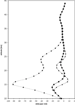
EGU 5.2.4 Sensitivity Study

To check the validity of the underlying assumptions and approximations, two sensitivity tests were carried out with simulated profiles. As reference profile we used a typical tropical H2O profile as shown in Fig.6 and a corresponding HDO profile that had the

isotopic composition of the VSMOW, thus an enrichment of 0 ‰. The corresponding

5

retrieval result is shown in Fig.7, which shows that for this single profile retrieval we obtain a resulting profile with an averageδD value of –4 ‰ (thus very close to 0 ‰)

and moderate oscillations smaller than 20 ‰ in the lower stratosphere.

In the first sensitivity test we then added 3 sharp positive 20 % perturbations at 14, 17 and 25 km (see Fig.6) on the total water vapor profile, i.e., for all isotopologues.

10

The retrieval reproduced the higher total water content due to these spikes, but strongly smoothed out the spikes according to the limited altitude resolution (not shown). The isotopic fractionation, however, changed by less than 10 ‰ (Fig.7). This result confirms that no significant artifacts in the isotopic fractionation profiles due to smoothing error propagation are to be expected and that the strategy to use equally resolved profiles

15

for ratio calculation is sufficiently robust. This is particularly remarkable considering the fact that the 20 % perturbations applied are large compared to natural total water variations and the 10 ‰ response of inferred δD values is much smaller than the

expected and observedδD variations.

In the second sensitivity study we applied the retrieval to perturbations as described

20

above to all water isotopologues except HDO. This implies that the input signal was isotopically strongly depleted at the height levels of the disturbances where 20 % more H16₂ O was artificially added (Fig. 6). The resulting δD profiles (Fig. 7) show a clear response to this perturbation. However, as expected the perturbation is smoothed out according to the actual altitude resolution of the retrieved HDO and H₂O profiles. In

25

fact, the two peaks at 14 and 17 km altitude cannot be resolved with our altitude reso-lution and are retrieved as one broad structure. On averageδD values are decreased

(17)

ACPD

Full Screen / Esc

EGU this broad structure we see the response to the second perturbation at 25 km altitude,

which is clearly resolved by the retrieval. Over the altitude range 10 to 30 km where we observe a response to the perturbation, the average enrichment is ≈ –35 ‰. This integrated response compares well with the input signal, where H16₂ O was disturbed by –200 ‰ at 3 out of 21 altitude levels, which corresponds to an average perturbation of

5

–29 ‰.

5.3 Total Error ofδD-Profiles

Figure 5a shows the representativeδD profile and the associated errors. At first we

note the important contribution of the parameter error: In the HDO and H₂O case the parameter error had a share of ≈ 20 to 30 %. In the δD case this is very similar which is

10

a consequence of the strong influence of the uncorrelated spectroscopic errors of HDO and H₂O. Thus, we obtain a height dependent total parameter error profile with values between 46 and 188 ‰. The noise error has a magnitude of 15 to 112 ‰. Together this leads to a height dependent total error for a singleδD profile in the range between

80 ‰ (11 km) and 195 ‰ (14 km). Most values are between 90 and 145 ‰.

15

6 Averaging

Envisat performs 14 orbits per day. As longitudinal variability in the stratosphere is generally much smaller than latitudinal variability, we have averaged all H₂O and HDO measurements by longitude and calculated dailyδD profiles. At each altitude level i the

random error of the average, i.e., the noise error and random parts of the parameter

er-20

ror, is reduced by a factor of 1/√Ni, whereNi is the number of profile values at altitude

i which were actually used for averaging. The retrieval algorithm identifies problematic

measurements, e.g., measurements affected by clouds, and excludes them from the ongoing calculation. This leads to the altitude dependence ofNi as shown in Table3.

From Figs.2b and1b the estimated reduction of the total error due to averaging is

vis-25

(18)

ACPD

Full Screen / Esc

EGU ible for the representative individual HDO and H₂O profiles. In the lower stratosphere

below 20 km random errors dominate the error budget for both species and averaging leads to a strong improvement in the total error. In the case of H2O, above 20 km the

parameter error components dominate the error profile and averaging leads to marginal improvement of the total error only. For HDO, the random errors are still the most

im-5

portant part of the error in this region, and the total error is strongly reduced by the averaging. After averaging, the total random errors are only dominating below 15 km, thus further averaging will not significantly reduce the errors at higher altitudes. Here the improvement of the spectroscopic uncertainty portion of the parameter error is the key to improving the total error.

10

The theoretically derived errors as estimated above (’estimated errors’) are compared to the actually derived variability of averaged HDO and H2O profiles, quantified in terms

of the standard deviation of the ensemble

σens =

s_P

n=1,Ni(xi,n− ¯xi) 2

N_i _{− 1} . (19)

and standard deviation of the mean

15 σmean= 1 pN_i s_P n=1,Ni(xi ,n− ¯xi) 2 Ni − 1 (20)

i is the height index and N denotes the number of the profile values used for averaging.

If the retrieved variability was much larger than the estimated error, this would either hint at underestimated errors or large natural variability within the ensemble, for exam-ple due to longitudinal variations. The standard deviation and the standard deviation of

20

the mean H2O and HDO profiles are shown in Fig. 1c and 2c. The magnitude of the

standard deviation of the mean is in good agreement with the random component of the estimated total error of the averaged profiles, with the exception of the two lowest altitudes (Figs. 1b and 2b). Using Eq.19 we also calculated the standard deviation

(19)

ACPD

Full Screen / Esc

EGU of the ensemble for δD (Fig. 5c). Again, the good agreement between the

theoreti-cally estimated total error (Fig.5a) and the standard deviation of the ensemble shows that the error estimation is sufficiently conservative and that the ensemble variability is small enough for meaningful averaging.

6.1 Latitudinal and vertical distribution of H2O

5

In the zonal mean, water shows the expected distribution that has been established in numerous studies carried out in the past (e.g. (Randel et al.,2001)): For 13 January 2003 we observe values>100 ppm in the troposphere, which decrease rapidly towards

the tropopause (Fig.8) due to decreasing temperatures. Values between 3 and 5 ppm are observed in the tropopause region and lower stratosphere (Fig.8) and the minimum

10

is located at the tropical tropopause of the winter hemisphere. A secondary minimum at around 23 km in the tropical stratosphere indicates the upward propagation of the seasonal cycle as part of the atmospheric tape recorder effect (Mote et al.,1996). In the stratosphere, H2O levels increase again with increasing altitude and latitude up to

values of about 7.5 ppm at the top of the shown height range. This shows the in situ

15

production of H2O from CH4oxidation, which increases as air ages in the stratospheric

circulation. In the cold Arctic winter vortex, we observe air from higher altitudes with high water content descending into the stratosphere down to 25 km. Deviations of our averaged water profiles retrieved with limited vertical resolution from validated water retrievals of better altitude resolution (Milz et al.,2005) do generally not exceed 1 ppm

20

when looking at annual averages. Occasionally, larger differences (up to 2 ppm) oc-cur at the tropopause. In the present case there is such a feature at 10◦ _{S. However,}

close to the tropopause larger deviations are expected due to strong vertical gradients both in H₂O and HDO there. Also, the artificially reduced height resolution of our H₂O retrievals (to match the altitude resolution of HDO) compared toMilz et al.(2005)

in-25

fluences the quality of the results. Thus, these deviations are intrinsic to our retrieval approach.

For the day of our retrieval, the retrieved profiles suggest a sharp hygropause, particu-948

(20)

ACPD

Full Screen / Esc

EGU larly in the region around 65◦ _{S. Such a sharp hygropause cannot be resolved by}

MI-PAS, and it leads to oscillations above the hygropause which produce an artificial H2O

minimum there. Those oscillations also lead to unusually high variability in this region, and indeed the standard deviation shows a pronounced maximum there. Therefore, this structure is excluded from further examination.

5

6.2 Latitudinal and vertical distribution of HDO

Figure9shows the zonal mean distribution of HDO on 13 January 2003. The general distribution of HDO, i.e., its increase above the tropopause as well as the general latitudinal shape, is similar to that of H2O, which reflects the fact that both species

have a common in situ source in the stratosphere i.e. oxidation of CH4 and H2. The

10

HDO minimum at the northern tropical tropopause corresponds to the H₂O minimum with values of approximately 0.2 ppb. Corresponding to H2O we observe a secondary

minimum in the tropical stratosphere around 23 km also for HDO. The descent of air in the winter vortex is amplified in HDO compared to H₂O, because the descending water is strongly enriched in deuterium. As a general characteristic, the HDO contours

15

are less smooth than those of H2O. As noted for H2O, the HDO minimum at 60–70◦S

and 13 km altitude is caused by the sharp retrieved hygropause and is not statistically significant. The standard deviation of the negative HDO values reach up to 250 % in this region. This negative artifact causes a positive compensating feature in the layer above at 15–17 km altitude.

20

6.3 Latitudinal and vertical distribution ofδD

TheδD value quantifies the ratio of HDO and H2O and it therefore highlights the

differ-ences in the general behavior of the two species. If changes in HDO perfectly mirrored changes in H₂O in the stratosphere, Fig. 10 would show constant values throughout the stratosphere. However, we observe an increase in δD with altitude above the

25

(21)

ACPD

Full Screen / Esc

EGU This shows directly that H₂O derived from the oxidation of CH₄ and H₂ is isotopically

enriched relative to the H2O that is injected from the troposphere, in agreement with

the expectations and with results from earlier measurement and model results (Moyer et al.,1996;Zahn et al., 2006; Johnson et al., 2001a; Stowasser et al., 1999; Rins-land et al.,1991). However, here for the first time we see a full two dimensional plot

5

ofδD in the stratosphere. The data indicate lower near tropopause δD values in the

winter hemisphere compared to the summer hemisphere, from the tropics to the high latitudes (with the exception of the artificial structure at 60-70◦ _{S). A detailed scientific}

interpretation of all those structures will follow in a dedicated publication.

In this paper we have shown that the natural variations in stratosphericδD values can

10

be clearly resolved because they are larger than the total errors derived above. As shown in Fig.5b, the estimated total error of an averagedδD profile reduces to values

between 35 ‰ (11 km) and 110 ‰ (36 km) when the noise part of the total error has been reduced by a factor of 1/pN_i. Most values are around 80 ‰. The estimated total random error for the averagedδD profiles is below 42 ‰ for all heights with a minimum

15

of 16 ‰ (18 km) and a maximum of 41 ‰ (14 km). In comparison, the natural variations recorded in the MIPAS data span several hundred ‰.

The MIPAS measurements thus provide a unique data set that will enable us to study various parts of the stratospheric water cycle in unprecedented detail. Because of the limited vertical resolution we are not able to resolve individual small scale processes

20

(< 4 km) like convective updraft that might also affect the isotopic fractionation of water

in the stratosphere (Webster and Heymsfield, 2003). However, their large scale rel-evance may well be assessed, and for the global stratospheric water cycle, this may even be the more important information.

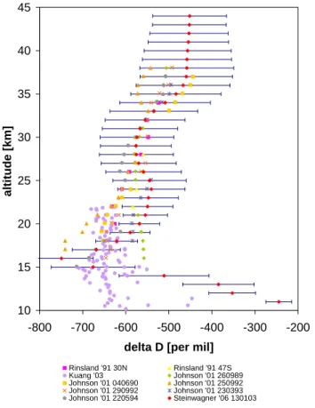
6.3.1 Comparison to other data sets

25

Figure 11 shows a comparison of our MIPAS retrievals to published values from the literature (Rinsland et al.,1991;Kuang et al.,2003;Johnson et al.,2001a). The general trends in the stratosphere from the earlier studies are captured by the MIPAS data.

(22)

ACPD

Full Screen / Esc

EGU Perfect agreement cannot be expected, because

1. our profile was actually taken in the tropics with colder tropopause temperatures compared to theJohnson et al.(2001a) data that were obtained at 33◦_{N and the}

Rinsland et al.(1991) data obtained at 30◦_{N and 47}◦_N;

2. the earlier recorded profiles were obtained at different times of the year and

dif-5

ferences could be due to a possible seasonal effect and

3. near the tropopause both HDO and H2O have strong gradients, which can

poten-tially cause averaging problems when the vertical resolution is limited.

Below the tropopause, ourδ values are more enriched than most of the (Kuang et al., 2003) data. However, large variability in the upper troposphere was recently reported

10

from in situ measurements (Webster and Heymsfield,2003). Overall, the vertical struc-ture, in particular the increase ofδD with altitude above the point of minimum

temper-ature, is in good agreement with the available data.

7 Conclusions

We have shown that MIPAS limb emission spectra can be used to investigate the

iso-15

topic composition of water vapor in the stratosphere on a global scale. HDO and H2O

profiles are retrieved in a multi target retrieval using the microwindow approach. In order to avoid artifacts in the resultingδD profiles both HDO and H₂O are retrieved at the same altitude resolution. A thorough error analysis is carried out to evaluate and distinguish noise and parameter errors. In the HDO/H2O ratio a considerable fraction

20

of the parameter error cancels out, and the resulting δD profiles are dominated by

spectroscopic uncertainties, resulting in a total error for single profiles of the order of 80 ‰ (11 km) to 195 ‰ (14 km) with most values between 90 and 145 ‰. The random component of the estimated total error can strongly be reduced by taking averages over multiple orbits on a single day. Thus, random errors are no longer limiting the

(23)

ACPD

Full Screen / Esc

EGU measurement precision for one day averaging. The estimated total error of the

av-eraged profiles (including spectroscopic uncertainties) is between 35 ‰ (11 km) and 110 ‰ (36 km). The random component of the total error is below 42 ‰ at all heights. The precision and altitude resolution of these zonal mean profiles is sufficient to study fractionation processes on a large scale, e.g. the principle role of different stratospheric

5

dehydration mechanisms, or in situ formation from methane oxidation. Thus the MIPAS measurements will provide unique information about the stratospheric water cycle.

Acknowledgements. This work was carried out as part of the AFO2000 project ISOSTRAT (07ATC01) funded by the German Ministry for Education and Research (BMBF). We thank ESA for access to the data.

10

References

Carlotti, M.: Global–fit approach to the analysis of limb–scanning atmospheric measurements, Appl. Opt., 27, 3250–3254, 1988. 934

Coffey, M. T., Hannigan, J., and Goldman, A.: Observations of upper troposheric/lower strato-spheric water vapor and its isotopes, J. Geophys. Res., 111, doi:10.1029/2005JD006093,

15

2006. 933

Dessler, A. E. and Sherwood, S. C.: A model of HDO in the tropical tropopause layer, Atmos. Chem. Phys., 3, 2173–2181, 2003,

http://www.atmos-chem-phys.net/3/2173/2003/. 933

Echle, G., von Clarmann, T., Dudhia, A., Flaud, J.-M., Funke, B., Glatthor, N., Kerridge, B.,

20

Lopez-Puertas, M., Martn-Torres, F. J., and Stiller, G. P.: Optimized Spectral Microwindows for Data Analysis of the Michelson Interferometer for Passive Atmospheric Sounding on the Environmental Satellite, Applied Optics, 39, Issue 30, 5531–5540, 2000. 935

Fischer, H., Blom, C., Oelhaf, H., Carli, B., Carlotti, M., Delbouille, L., Ehhalt, D., Flaud, J.-M., Isaksen, I., Lopez-Puerta, J.-M., McElroy, C.T., and Zander, R., 2000, Envisat-Mipas, the

25

Michelson Interferometer for Passive Atmospheric Sounding; An instrument for atmospheric chemistry and climate research, ESA SP-1229, C. Readings and R. A. Harris, eds. (Euro-pean Space Agency, Noordwijk, The Netherlands), 2000. 933

(24)

ACPD

Full Screen / Esc

EGU

Fischer, H.: Remote Sensing of Atmospheric Trace Gases, Interdisciplinary Science Reviews, Vol. 18, p. 185–191, 1993.933

Flaud, J.-M., Piccolo, C., Carli, B., Perrin, A., Coudert, L. H., Teffo, J.-L., and Brown, L. R.: Molecular line parameters for the MIPAS (Michelson Interferometer for Passive Atmospheric Sounding) experiment, Atmos. Oceanic Opt., 16, 172–182, 2003. 934

5

Franz, P. and R ¨ockmann, T.: High-precision isotope measurements of H16₂ O, H17₂ O, H18₂ O, and the D17O-anomaly of water vapor in the southern lowermost stratosphere, Atmos. Chem. Phys. Discuss., pp. 5373–5403, 2005. 933

F ¨uglistaler, S. and Haynes, P. H.: Control of interannual and longer-term variability of strato-spheric water vapor, J. Geophys. Res., 110, doi:10.1029/2005JD006019, 2005. 932

10

Holton, J. R. and Gettelmann, A.: Horizontal transport and the dehydration of the stratosphere, Geophys. Res. Lett., 28(14), 2799–2802, 2001. 932

Irion, F. W., Moyer, E. J., Gunson, M. R., Rinsland, C. P., Michelson, H. A., Salawitch, R. J., Yung, Y. L., Chang, A. Y., Newchurch, M. J., Abbas, M. M., Abrams, M. C., and Zander, R.: Stratospheric observations of CH₃D and HDO from ATMOS infrared solar spectra:

Enrich-15

ments of deuterium in methane and implications for HD, Geophys. Res. Lett., 23, 2381–2384, 1996. 933

Johnson, D. G., Jucks, K. W., Traub, W. A., and Chance, K. V.: Isotopic composition of strato-spheric water vapor: Implications for transport, J. Geophys. Res., 106(D11), 12 219–12 226, 2001a.933,950,951,970

20

Johnson, D. G., Jucks, K. W., Traub, W. A., and Chance, K. V.: Isotopic composition of stratospheric water vapor: Measurements and photochemistry, J. Geophys. Res., 106(D11), 12 211–12 217, 2001b.933

Kuang, Z., G. C, T., Wenneberg, P. O., and Yung, Y. L.: Measured HDO/H₂O ratios across the tropical tropopause, Geophys. Res. Lett., 30(7), 1372, doi:10.1029/2003GL017023, 2003.

25

950,951,970

Lautie, N., Urban, J., and Group, O. R.: Odin/SMR limb observations of stratospheric water vapor and its isotopes., EGS - AGU - EUG Joint Assembly, Abstracts from the meeting held in Nice, France, 6 - 11 April 2003, abstract #7320, pp. 7320–+, 2003. 933

Milz, M., von Clarmann, T., Fischer, H., Glatthor, N., Grabowski, U., H ¨opfner, M., Kellmann,

30

S., Kiefer, M., Linden, A., Mengistu Tsidu, G., Steck, T., Stiller, G. P., Funke, B., L ´opez-Puertas, M., and Koukouli, M. E.: Water Vapor Distributions Measured with the Michelson Interferometer for Passive Atmospheric Sounding on board Envisat (MIPAS/Envisat), 2005.

(25)

ACPD

Full Screen / Esc

EGU

935,940,948

Mote, P. W., Rosenlof, K., McIntyre, M., Carr, E. S., Gille, J. C., Holton, J. R., Kinnersley, J. S., Pumphrey, H. C., III, J. M. R., and Waters, J. W.: An atmospheric tape recorder: The imprint of tropical tropopause temperatures on stratospheric water vapor, Journal of Geophysical Research, 101, 2989–4006, 1996. 948

5

Moyer, E. J., Irion, F. W., Yung, Y. L., and Gunson, M. R.: ATMOS stratospheric deuterated water and implications for troposhere-stratosphere transport, Geophys. Res. Lett., 23, 2385–2388, 1996. 933,942,950

Payne, V., Dudhia, A., and Piccolo, C.: Isotopic Measurements of Water Vapour and Methane from the MIPAS Satellite Instrument, AGU Fall Meeting Abstracts, pp. B733+, 2004. 944

10

Pollock, W., Heidt, L., Lueb, R., and Ehhalt, D.: High-precision isotope measurements of H216O, H217O, H218O, and the D17O-anomaly of water vapor in the southern lowermost stratosphere, J. Geophys. Res., pp. 5555–5568, 1980. 933

Randel, W. J., Wu, F., Gettelman, A., III, J. R., Zawodny, J. M., and Oltmans., S. J.: Seasonal variation of water vapor in the lower stratosphere observed in Halogen Occultation

Experi-15

ment data, J. Geophys. Res., 106(D13), 14 313–14 325, 2001. 948

Remedios, J.: Extreme atmospheric constituent profiles for MIPAS, 1999. Proceedings of ESAMS ’99 - European Symposium on Atmospheric Measurements from Space, pages 779-782, 1999.935

Rinsland, C. P., Gunson, M. R., Foster, J. C., Toth, R. A., Farmer, C. B., and Zander, R.:

20

Stratospheric profiles of heavy water vapor isotopes and CH₃D from analysis of the ATMOS Spacelab-3 infrared solar spectra, Geophys. Res. Lett., 96(D1), 1057–1068, 1991.933,950, 951,970

Rodgers, C. D.: Inverse Methods for Atmospheric Sounding: Theory and Practice, World Sci-entific, ISBN 981022740X, 256 pages, Oxford, 2000. 935,937

25

Rosenlof, K. H., Chiou, E.-W., Chu, W. P., Johnson, D. G., Kelly, K. K., Michelsen, H. A., Nedoluha, G. E., Remsberg, E. E., Toon, G. C., and McCormick, M. P.: Stratospheric water vapor increases over the past half-century, Geophys. Res. Lett., 28, 1195–1198, doi:10. 1029/2000GL012502, 2001. 932

Rothman, L. S., Barbe, A., Benner, D. C., Brown, L. R., Camy-Peyret, C., Carleer, M. R.,

30

Chance, K., Clerbaux, C., Dana, V., Devi, V. M., Fayt, A., Flaud, J.-M., Gamche, R. R., Goldman, A., Jacquemart, D., Jucks, K. W., Lafferty, W. J., Mandin, J.-Y., Massie, S. T., Nemtchinov, V., Newnham, D. A., Perrin, A., Rinsland, C. P., Schroeder, J., Smith, K. M.,

(26)

ACPD

Full Screen / Esc

EGU

Smith, M. A. H., Tang, K., Toth, R. A., Vander Auwera, J., Varanasi, P., and Yoshino, K.: The HITRAN molecular spectroscopic database: edition of 2000 including updates through 2001, J. Quant. Spectrosc. Radiat. Transfer, 82, 5–44, doi:10.1016/S0022-4073(03)00146-8, 2003. 934,935

Schneider, M., Hase, F., and Blumenstock, T.: Ground-based remote sensing of HDO/H₂O ratio

5

profiles: Introduction and validation of an innovative retrieval approach, Atmos. Chem. Phys. Discuss., 06, 5269–5327, 2006,

http://www.atmos-chem-phys-discuss.net/06/5269/2006/. 944

Sherwood, S. C. and Dessler, A. E.: On the control of stratospheric humidity, Geophys. Res. Lett., 27(16), 2513–2516, 2000. 932

10

Smith, J. A., Ackerman, A. S., Jensen, E. J., and Toon, O. B.: Role of deep convection in establishing the isotopic compsition of water vapor in the tropical transition layer, Geophys. Res. Lett., 33, 2006. 933

Stiller, G. P.: The Karlsruhe optimized and precise radiative transfer algorithm (KOPRA), Wis-senschaftliche Berichte, FZKA 6487, 2000. 934

15

Stowasser, M., Oelhaf, H., Wetzel, G., Friedl-Vallon, F., Maucher, G., Seefeldner, N., Tri-eschmann, O., von Clarmann, T., and Fischer, H.: Simultaneous measurements of HDO, H₂O and CH₄with MIPAS-B: Hydrogen budget and indication of dehydration inside the polar vortex, J. Geophys. Res., 104(D16),19, 19 213–19 225, 1999.933,950

Tikhonov, A.: On the solution of incorrectly stated problems and a method of regularization,

20

Dokl. Acad. Nauk SSSR, 151, 501–504, 1963.934

von Clarmann, T., Glatthor, N., Grabowski, U., H ¨opfner, M., Kellmann, S., Kiefer, M., Linden, A., Tsidu, G. M., Milz, M., Steck, T., Stiller, G. P., Wang, D. Y., Fischer, H., Funke, B., Gil-Lpez, S., and Lpez-Puertas, M.: Retrieval of temperature and tangent altitude pointing from limb emis-sion spectra recorded from space by the Michelson Interferometer for Passive Atmospheric

25

Sounding (MIPAS), J. Geophys. Res., 108, No. D23, 4736, doi:10.1029/2003JD003602, 2003. 934,936

Webster, C. R. and Heymsfield, A. J.: water isotope ratios D/H, O-18/O-16, O-17/O-16 in and out of cloudsmap dehydration pathways, Science, 302(5651), 1742–1745, 2003. 933,950, 951

30

Worden, J. R., Bowman, K., and Noone, D.: TES Observations of the Isotopic composition of Tropospheric Water Vapor, AGU Fall Meeting Abstracts, pp. C3+, 2005. 944

(27)

strato-ACPD

Full Screen / Esc

EGU

spheric tracer (SF6) ages, and water vapor isotope (D, T) tracers, J. Atmos. Chem, 39, 2001. 933

Zahn, A., Barth, V., Pfeilsticker, K., and Platt, U.: Deuterium, oxygen-18, and tritium as tracers for water vapour transport in the lower stratosphere and tropopause region, J. Atmos. Chem, 30, 1998. 933

5

Zahn, A., Franz, P., Bechtel, C., Grooss, J.-U., and R ¨ockmann, T.: Modelling the budget of mid-dle atmospheric water vapour isotopes, Atmos. Chem. Phys. Discuss., 1680–7324/acp/2006-6-2073, 2073–2090, 2006. 933,950

(28)

ACPD

Full Screen / Esc

EGU

Table 1. Microwindows used in the HDO measurements of MIPAS.

Microwindow Left border [cm−1_] _{Right border [cm}−1_]

1 1250.2000 1253.1750 2 1272.9000 1273.7000 3 1286.5000 1288.1750 4 1358.2250 1361.0500 5 1364.5750 1365.9250 6 1370.7500 1373.1500 7 1410.4250 1413.4000 8 1421.0500 1424.0250 9 1424.1750 1427.1500 10 1432.9500 1435.9250 11 1449.6250 1452.6000 12 1452.8500 1455.2500 13 1467.6750 1470.6250 14 1479.4750 1482.4500

(29)

ACPD

Full Screen / Esc

EGU

Table 2. Assumed 1σ parameter uncertainties used in the error calculation.

perturbed quantity value and unit

SO₂ 10–37 km: 10−3_{ppm, above 37 km 10}−5_ppm

T 2 K (constant over height) Hor. T gradient (lat) 0.01 K/km (constant over height) ils 3% at 600 and 1600 cm−1

los 0.15 km

spectral shift 0.0005 cm−1

gain 1 %

(30)

ACPD

Full Screen / Esc

EGU

Table 3. Number of measurements per height step taken into account for averaging, for the measurements on 13 January 2003 between 7.5◦_{N and 12.5}◦_N.

Altitude(s) [km] Number of measurements

11 9 12 9 13 15 14 16 15 16 16 18 17 22 18 23 19 26 20–44 28

(31)

ACPD

Full Screen / Esc

Printer-friendly Version Interactive Discussion EGU 10 15 20 25 30 35 40 45 0 1 2 3 4 5 6 7 8 c) b) a)

H2O profile with total error

total error noise error parameter error total random error

a lt it u d e ( k m ) 10 15 20 25 30 35 40 45

av. H2O profile with total error

total error of av. profile noise error of av. profile param. error of av. profile tot. rand. error of av. profile

a lti tu d e ( k m ) 0 1 2 3 4 5 6 7 8 10 15 20 25 30 35 40 45 av. H2O profile

stdev of averaged profiles sterr of av. profile total random error of av. profile

a lt it u d e ( k m ) [H₂O] (ppm)

Fig. 1. (a) (top) H₂O profile retrieved from MIPAS spectra measured on 13 January 2003 at

12◦_{N and 28}◦_{W together with total error bars, noise errors, parameter errors and total random}

errors. (b) (middle) Zonal mean (7.5◦_N–12_.5◦_{N) H}

2O profile on 13 January 2003 with estimated

errors. (c) (bottom) Standard deviation for the H₂O profile (“standard deviation of averaged profiles”) and and standard deviation of the zonal mean H₂O profiles (“sterr of av. profile”).

(32)

ACPD

Full Screen / Esc

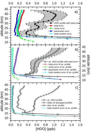
Printer-friendly Version Interactive Discussion EGU 10 15 20 25 30 35 40 45 0.0 0.2 0.4 0.6 0.8 1.0 1.2 1.4 1.6 c) a)

HDO profile with total error total error

noise error parameter error total random error

a lt it u d e ( k m ) 10 15 20 25 30 35 40 45

av. HDO profile with total error total error of av. profile noise error of av. profile parameter error of av. profile total random error of av. profile

a lti tu d e ( k m ) 0.0 0.2 0.4 0.6 0.8 1.0 1.2 1.4 1.6 10 15 20 25 30 35 40 45 b)

av. HDO profile stdev of averaged profiles sterr of av. profile total random error of av. profile

a lt it u d e ( k m ) [HDO] (ppb)

Fig. 2. (a) (top) HDO profile retrieved from MIPAS spectra measured on 13 January 2003 at 12◦_{N and 28}◦_{W together with total error bars, noise errors, parameter errors and total random}

errors. (b) (middle) Zonal mean (7.5◦_N–12_.5◦_{N) HDO profile on 13 January 2003 with}

esti-mated errors. (c) (bottom) Standard deviation for the HDO profile and and standard deviation of the zonal mean HDO profiles.

(33)

ACPD

Full Screen / Esc

Printer-friendly Version Interactive Discussion EGU -0.2 0.0 0.2 0.4 0.6 Averaging kernel 0 20 40 60 80 A l t i t u d e [ k m ] -0.2 0.0 0.2 0.4 0.6 Averaging kernel 0 20 40 60 80 A l t i t u d e [ k m ]

Fig. 3. (a) Columns of the averaging kernel of H₂O (left) and (b) HDO (right).

(34)

ACPD

Full Screen / Esc

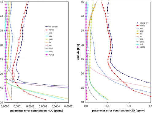
Printer-friendly Version Interactive Discussion EGU 10 15 20 25 30 35 40 45 0,0000 0,0001 0,0002 0,0003 0,0004 0,0005

parameter error contribution HDO [ppmv]

a lt it u d e [ k m ]

tot par err hitmid tem tgra gain ils los SO2 shift N2O5 45 10 15 20 25 30 35 40 45 0,0 0,5 1,0 1,5

parameter error contribution H2O [ppmv]

a lt it u d e [ k m]

tot par err hitmid tem gain ils los tgra SO2 shift N2O5

Fig. 4. Contributions of the single parameter errors to the total parameter error for (a) (left) HDO and (b) (right) H₂O.

(35)

ACPD

Full Screen / Esc

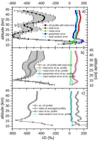
Printer-friendly Version Interactive Discussion EGU 10 15 20 25 30 35 40 45 -800 -600 -400 -200 0 200 a)

D profile with total error total error

noise error parameter error total random error

a lt it u d e ( k m ) 10 15 20 25 30 35 40 45 b)

av. D profile with total error total error of av. profile noise error of av. profile parameter error of av. profile total random error of av. profile

a lti tu d e ( k m ) -800 -600 -400 -200 0 200 10 15 20 25 30 35 40 45 c) av. D profile stdev of averaged profiles sterr of av. profile total random error of av. profile

a lt it u d e ( k m ) D (‰)

Fig. 5. (a) (top)δD profile retrieved from MIPAS spectra measured on 13 January 2003 at 12◦_N

and 28◦_{W together with total error bars, noise errors, parameter errors and total random errors.}

(b) (middle) Zonal mean (7.5◦_N–12_.5◦_N)_{δD profile on 13 January 2003 with estimated errors.}

(c) (bottom) Standard deviation for theδD profile and and standard deviation of the zonal mean

(36)

ACPD

Full Screen / Esc

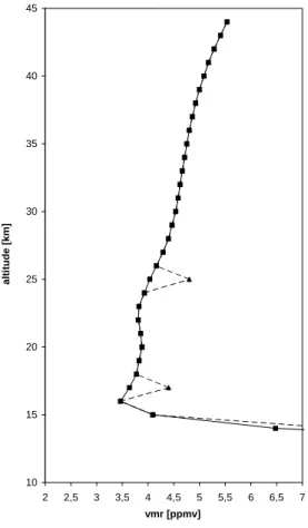
Printer-friendly Version Interactive Discussion EGU 10 15 20 25 30 35 40 45 2 2,5 3 3,5 4 4,5 5 5,5 6 6,5 7 vmr [ppmv] a lt it u d e [ k m ]

Fig. 6. H₂O input profile for sensitivity study. We introduced artificial spikes of +20% at 14,

17 and 25 km altitude either only to the total water profile (all isotopologues) or to all water isotopologues but HDO

(37)

ACPD

Full Screen / Esc

Printer-friendly Version Interactive Discussion EGU 10 15 20 25 30 35 40 45 -100 -90 -80 -70 -60 -50 -40 -30 -20 -10 0 10 20

delta [per mil]

a lt it u d e [ k m ]

Fig. 7. Inferred δD profiles from the sensitivity study. Sqares, solid line: no perturbation

(reference); triangles, dashed line: total water perturbed (+20 % at 14, 17 and 25 km); dots, dotted line: all water isotopes but HDO perturbed (+20 % at 14, 17 and 25 km). When total water is perturbed, the profiles do not deviate substantially. When HDO is perturbed, the total shift in the isotope ratio in the input profile is well recovered by a shift in theδ value that varies with height. Perturbation spikes are smeared out due to the limited vertical resolution.

(38)

ACPD

Full Screen / Esc

EGU

Fig. 8. Zonal mean distribution of H₂O 13 January 2003, measured by MIPAS. 9 to 28

mea-surements were taken into account for averaging at each altitude and latitude level (see Table3 for details).

(39)

ACPD

Full Screen / Esc

EGU

Fig. 9. Zonal mean distribution of HDO for 13 January 2003, measured by MIPAS, 9 to 28 measurements were taken into account for averaging at each altitude and latitude level (see Table3for details).

(40)

ACPD

Full Screen / Esc

EGU

Fig. 10. Zonal mean distribution ofδD, 13 January 2003, inferred from averaged HDO and