HAL Id: cea-03174102
https://hal-cea.archives-ouvertes.fr/cea-03174102
Submitted on 18 Mar 2021
HAL is a multi-disciplinary open access
archive for the deposit and dissemination of
sci-entific research documents, whether they are
pub-lished or not. The documents may come from
teaching and research institutions in France or
abroad, or from public or private research centers.
L’archive ouverte pluridisciplinaire HAL, est
destinée au dépôt et à la diffusion de documents
scientifiques de niveau recherche, publiés ou non,
émanant des établissements d’enseignement et de
recherche français ou étrangers, des laboratoires
publics ou privés.
The infrared-radio correlation of star-forming galaxies is
strongly M⋆-dependent but nearly redshift-invariant
since z
∼ 4
I. Delvecchio, E. Daddi, M. T. Sargent, M. J. Jarvis, D. Elbaz, S. Jin, D. Liu,
I. H. Whittam, H. Algera, R. Carraro, et al.
To cite this version:
I. Delvecchio, E. Daddi, M. T. Sargent, M. J. Jarvis, D. Elbaz, et al.. The infrared-radio correlation of
star-forming galaxies is strongly M⋆-dependent but nearly redshift-invariant since z
∼ 4. Astronomy
and Astrophysics - A&A, EDP Sciences, 2021, 647, pp.A123. �10.1051/0004-6361/202039647�.
�cea-03174102�
https://doi.org/10.1051/0004-6361/202039647 c I. Delvecchio et al. 2021
Astronomy
&
Astrophysics
The infrared-radio correlation of star-forming galaxies is strongly
M
?
-dependent but nearly redshift-invariant since z
∼
4
I. Delvecchio
1,2, E. Daddi
1, M. T. Sargent
3, M. J. Jarvis
4,5, D. Elbaz
1, S. Jin
6,7, D. Liu
8, I. H. Whittam
4,5, H. Algera
9,
R. Carraro
10, C. D’Eugenio
1, J. Delhaize
11, B. S. Kalita
1, S. Leslie
9, D. Cs. Molnár
12, M. Novak
8, I. Prandoni
13,
V. Smolˇci´c
14, Y. Ao
15,16, M. Aravena
17, F. Bournaud
1, J. D. Collier
18,19, S. M. Randriamampandry
20,21,
Z. Randriamanakoto
20, G. Rodighiero
22, J. Schober
23, S. V. White
24, and G. Zamorani
25(Affiliations can be found after the references) Received 11 October 2020/ Accepted 22 January 2021
ABSTRACT
Over the past decade, several works have used the ratio between total (rest 8−1000 µm) infrared and radio (rest 1.4 GHz) luminosity in star-forming galaxies (qIR), often referred to as the infrared-radio correlation (IRRC), to calibrate the radio emission as a star formation rate (SFR) indicator.
Previous studies constrained the evolution of qIRwith redshift, finding a mild but significant decline that is yet to be understood. Here, for the first
time, we calibrate qIRas a function of both stellar mass (M?) and redshift, starting from an M?-selected sample of >400 000 star-forming galaxies
in the COSMOS field, identified via (NUV − r)/(r − J) colours, at redshifts of 0.1 < z < 4.5. Within each (M?,z) bin, we stacked the deepest available infrared/sub-mm and radio images. We fit the stacked IR spectral energy distributions with typical star-forming galaxy and IR-AGN templates. We then carefully removed the radio AGN candidates via a recursive approach. We find that the IRRC evolves primarily with M?, with more massive galaxies displaying a systematically lower qIR. A secondary, weaker dependence on redshift is also observed. The best-fit analytical
expression is the following: qIR(M?, z) = (2.646 ± 0.024) × (1+z)(−0.023±0.008)–(0.148 ± 0.013) × (log M?/M −10). Adding the UV dust-uncorrected
contribution to the IR as a proxy for the total SFR would further steepen the qIRdependence on M?. We interpret the apparent redshift decline
reported in previous works as due to low-M?galaxies being progressively under-represented at high redshift, as a consequence of binning only in
redshift and using either infrared or radio-detected samples. The lower IR/radio ratios seen in more massive galaxies are well described by their higher observed SFR surface densities. Our findings highlight the fact that using radio-synchrotron emission as a proxy for SFR requires novel M?-dependent recipes that will enable us to convert detections from future ultra-deep radio surveys into accurate SFR measurements down to
low-M?galaxies with low SFR.
Key words. galaxies: star formation – radio continuum: galaxies – infrared: galaxies – galaxies: active – galaxies: evolution
1. Introduction
For nearly fifty years, astronomers have studied the observed correlation between total infrared (IR; rest-frame 8−1000 µm, i.e. LIR) and radio (e.g., rest-frame 1.4 GHz, i.e. L1.4 GHz)
spec-tral luminosity arising from star formation, typically referred to as the ‘infrared-radio correlation’ (IRRC, e.g.,Helou et al. 1985;
de Jong et al. 1985). This tight (1σ ∼ 0.16 dex, e.g.,Molnár et al. 2021) correlation is often parametrised via the IR-to-radio lumi-nosity ratio qIR, defined as (e.g.,Helou et al. 1985; Yun et al. 2001): qIR= log LIR[W] 3.75 × 10¹²[Hz] ! − log(L1.4 GHz[W Hz−1]), (1)
where 3.75 × 10¹²Hz represents the central frequency over
the far-infrared (FIR, rest-frame 42−122 µm) domain, usually scaled to IR in the recent literature. In the Local Universe, the IRRC (or its parametrisation qIR) appears to hold over at
least three orders of magnitude in both LIR and L1.4 GHz (e.g.,
Helou et al. 1985; Condon 1992; Yun et al. 2001). Broadly
speaking, this is because the infrared emission comes from dust heated by fairly massive (&5 M ) OB stars, while radio emission
arises from relativistic cosmic ray electrons (CRe) accelerated by shock waves produced when massive stars (&8 M ) explode as
supernovae. Nevertheless, CRe are also subject to different cool-ing processes as they propagate throughout the galaxy, which are
mainly caused by inverse Compton, bremsstrahlung, and ionisa-tion losses (e.g.,Murphy 2009).
Surprisingly enough, despite all such processes at play, infrared and radio emission are observed to be correlated, both in local star-forming late-type galaxies and even in merging galax-ies (e.g.,Condon et al. 1993,2002;Murphy 2013). This has been a strong motivator for the use of radio-continuum emission as a dust-unbiased star formation rate (SFR) tracer also in the faint radio sky (e.g., Condon 1992; Bell 2003;Murphy et al. 2011,
2012). Moreover, measuring the offset from the IRRC has been widely used to indirectly identify radio-excess active galactic nuclei (AGN; e.g., Donley et al. 2005; Del Moro et al. 2013;
Bonzini et al. 2015;Delvecchio et al. 2017).
These applications, however, significantly rely on a proper understanding of whether and how the IRRC evolves over cos-mic time and across different types of galaxies. Despite its extensive application in extragalactic astronomy, the detailed physical origins of the IRRC and the nature of its cosmic evo-lution have long been debated (e.g., Harwit & Pacini 1975;
Rickard & Harvey 1984;de Jong et al. 1985;Helou et al. 1985;
Hummel et al. 1988;Condon 1992;Garrett 2002;Appleton et al. 2004;Murphy et al. 2008;Jarvis et al. 2010;Sargent et al. 2010;
Ivison et al. 2010a,b; Bourne et al. 2011; Smith et al. 2014;
Magnelli et al. 2015;Calistro Rivera et al. 2017;Delhaize et al.
2017; Gürkan et al. 2018; Molnár et al. 2018; Algera et al.
2020a).
Open Access article,published by EDP Sciences, under the terms of the Creative Commons Attribution License (https://creativecommons.org/licenses/by/4.0),
For example, some studies of local star-forming galaxies (SFGs), ranging from dwarf (e.g., Wu et al. 2008) to ultra-luminous infrared galaxies (ULIRGs; LIR > 1012L ; e.g., Yun et al. 2001) have concluded that the IRRC remains linear across a wide range of LIR. Conversely, other studies have argued that at
low luminosities the IRRC may break down, which is consistent with a non-linear trend of the form LIR ∝ L0.75−0.901.4 GHz (e.g.,Bell 2003;Hodge et al. 2008;Davies et al. 2017;Gürkan et al. 2018), which might be partly induced by dust heating from old stellar populations (Bell 2003).
Several models have attempted to explain this non linearity. On the one hand, calorimetric models assume that galaxies are optically thick in the ultraviolet (UV), so that UV emission is fully re-emitted in the IR; likewise, CRe radiate away their total energy through synchrotron emission before escaping the galaxy (e.g., Voelk 1989). These conditions might hold in the most massive (stellar mass M? & 1010M ) SFGs because of their
increasing compactness (i.e. the size-mass relation Re ∝ M0.22? ,
van der Wel et al. 2014), which might enhance their ability
to retain the gas ejected by stars. However, this is likely to break down towards lower M?galaxies due to smaller sizes and
lower obscuration (e.g.,Bourne et al. 2012). On the other hand, non-calorimetric models or the optically thin scenario (Helou & Bicay 1993; Niklas & Beck 1997; Bell 2003; Lacki et al. 2010) support the argument that several physical mechanisms cancel each other out, creating a sort of ‘conspiracy’ that keeps the IRRC unexpectedly tight and linear. Indeed, both IR and radio luminosities are expected to underestimate the total SFR in low M? and low-SFR surface density galaxies (Bell 2003), inducing a departure of the IRRC from linearity. This was not, however, observed in our study. Radio synchrotron models pos-tulate that such small galaxies are not able to prevent CRe from escaping, causing a global deficit of radio emission at a fixed SFR. Similarly, the IR domain becomes less sensitive to SFR in low-M?galaxies (e.g.,Madau & Dickinson 2014), generating an IR deficit of a similar amount, which might counterbalance the radio emission and keep the IRRC linear. Understanding the dis-crepancy between model predictions and observations is crucial, since the linearity (or not) of the IRRC has direct implications for using radio emission as a SFR tracer.
From an observational perspective, it is widely recognised that there is a tight relation linking SFR and M? in nearly all SFGs, namely, namely the ‘main sequence’ of star formation (MS, scatter ∼0.2−0.3 dex). This relation holds from z ∼ 5 down to the Local Universe (e.g.,Brinchmann et al. 2004;Noeske et al. 2007; Elbaz et al. 2011; Whitaker et al. 2012; Speagle et al. 2014; Schreiber et al. 2015; Lee et al. 2015), showing a flat-tening at high M?and an evolving normalisation with redshift.
Because the SFR is directly linked to LIR, especially in massive
SFGs (Kennicutt 1998), the existence of the MS gives an addi-tional argument that studying qIR as a function of M?could be
of the utmost importance for our understanding of what drives the IRRC in galaxies.
Recent studies have corroborated the idea that the IRRC slightly, but significantly, declines with redshift (Ivison et al.
2010b; Magnelli et al. 2015; Calistro Rivera et al. 2017;
Delhaize et al. 2017) in the form of qIR ∝ (1+ z)[−0.2:−0.1],
although the physical explanation for such an evolution is still uncertain. Somewhat different conclusions were reached by other works (e.g.,Garrett 2002;Appleton et al. 2004;Ibar et al. 2008; Jarvis et al. 2010; Sargent et al. 2010; Bourne et al. 2011) that ascribe this apparent evolution to selection effects; for instance, comparing flux-limited samples, each with a different selection function.
In this regard, we note that any selection method is sensitive to brighter, that is, more massive galaxies towards higher red-shifts. By binning in redshift, only a restricted range in galaxy M? becomes detectable at each redshift for any flux limited sample, thus inducing a bias as a function of z. Therefore, it is time to simultaneously examine the evolution of the IRRC as a function of M?and redshift. We emphasise that our approach is
fully empirical. However, a possible dependence of the IRRC on M? is expected from some synchrotron emission models (e.g., Lacki & Thompson 2010;Schober et al. 2017) and this might reflect some combination of the underlying physics originating the IRRC (see Sect.5).
The main goal of the present paper is to calibrate the IRRC, for the first time, as a function of both M? and redshift over a
broad range. To this end, we start from an M?-selected sample of >400 000 galaxies at 0.1 < z < 4.5 collected from deep Ultra-VISTA images in the Cosmic Evolution Survey (Scoville et al. 2007; centered at RA= +150.11916667; Dec = +2.20583333 (J2000)). Then we leverage the new de-blended far-IR/sub-mm data (Jin et al. 2018) recently compiled in COSMOS, which allow us to circumvent blending issues due to poor angular res-olution and measure LIR for typical MS galaxies out to z ∼ 4.
In addition, we exploit the deepest radio-continuum data taken from the VLA-COSMOS 3 GHz Large Project (Smolˇci´c et al.
2017a). Individual detections are combined with stacked flux
densities of non-detections, at both IR and radio frequencies to assess the average qIRas a function of M?and redshift.
The layout of this paper is as follows. A description of the sample selection and multi-wavelength ancillary data is given in Sect.2. We describe the stacking analysis in Sect.3, includ-ing measurements of LIR(Sect.3.1) and L1.4 GHz(Sect.3.4). The
average qIR as a function of M? and redshift is presented in
Sect.4, where we perform a careful subtraction of radio AGN at different M? via a recursive approach. Our main results are
discussed and interpreted in Sect. 5 within the framework of previous observational studies and theoretical models. The main conclusions are summarised in Sect.6. In addition, we test our total 3 GHz flux densities in AppendixA. A detailed compari-son between radio stacking results is presented in AppendixB. In AppendixC, we discuss how the final IRRC is sensitive to our AGN subtraction method. Finally, in AppendixDwe quan-tify how different assumptions from the literature would change our main results. Throughout this paper, magnitudes are given in the AB system (Oke 1974). We assume aChabrier(2003) initial mass function (IMF) and aΛCDM cosmology with Ωm= 0.30,
ΩΛ= 0.70, and H0= 70 km s−1Mpc−1(Spergel et al. 2003). 2. Multi-wavelength data and sample selection In this section, we describe the creation of a Ksprior catalogue,
which we used to select our parent sample in the COSMOS field. The COSMOS field (2 deg2) boasts an exquisite
photomet-ric data set, spanning from the X-rays to the radio domain1. The most recent collection of multiwavelength photometry comes from the COSMOS2015 catalogue (Laigle et al. 2016), which contains 1 182 108 sources extracted from a stacked Y JHKs
image (blue dots in Fig. 1). In particular, this catalogue joins optical photometry from Subaru Hyper-Suprime Cam (2 deg2;
Capak et al. 2007) and from the Canada-France-Hawaii
Tele-scope Legacy Survey (CFHT-LS, central 1 deg2; McCracken et al. 2001); the near-infrared (NIR) bands Y, J, H, and Ksfrom 1 An exhaustive overview of the COSMOS field is available at:http:
UltraVISTA DR2 (down to Ks <24.5 in the central 1.5 deg2, of
which 0.6 deg2 are covered by ultra-deep stripes with limiting
Ks < 25.2; McCracken et al. 2012), and from CFHT H and
Ks observations obtained with the WIRCam (Ks < 23.9
out-side the UltraVISTA area; McCracken et al. 2001). Over the full 2 deg2 area, mid-infrared (MIR) photometry was obtained from the Spitzer Large Area Survey with Hyper-Suprime-Cam (SPLASH;Steinhardt et al. 2014; Capak et al., in prep.) using 3.6−8 µm data from the Infrared Array Camera (IRAC). We refer the reader toLaigle et al.(2016) for more details.
In order to obtain a homogeneous galaxy selection function, we limited our study to the inner UltraVISTA DR2 area, while also excluding stars and masked regions from the COSMOS2015 catalogue with less accurate photometry, which reduces the ini-tial sample to 45% of its size (524 061 sources). Following Jin et al. (2018), we partly fill up these blank regions by adding 22 838 unmasked Ks–selected sources from the UltraVISTA
cat-alogue of Muzzin et al.(2013) (3σ limit of Ks < 24.35 with
200aperture). This ensures a more complete coverage within the UltraVISTA area, with fluctuations in the prior source density of only 2.5%. This builds on our Ks prior sample of 546 899
galaxies. Given the similar selection, we confirm that exclud-ing the slightly shallower ∼4% subsample from Muzzin et al.
(2013) leaves our results unchanged. Thus, we maintained them throughout this work.
Photometric redshifts and M?estimates were retrieved from the corresponding catalogues by fitting the optical-MIR photom-etry using the stellar population synthesis models of Bruzual & Charlot (2003). Both redshift and M? values represent the median of the corresponding likelihood distribution. Laigle et al.(2016) report an average photometric redshift accuracy of h|∆z/(1 + z)|i = 0.007 at z < 3, and 0.021 at 3 < z < 6. A similar accuracy of 0.013 is reached in the catalogue fromMuzzin et al.
(2013) at z < 4. We further inspected a subset of 5400 sources showing a skewed redshift probability distribution function (with &5% chance to be offset from the median by >0.5 × [1 + zp]).
However, we verified that removing such potential redshift inter-lopers does not have any impact on our results. As inJin et al.
(2018), publicly available spectroscopic redshifts were collected from the new COSMOS master spectroscopic catalogue (cour-tesy of M. Salvato, within the COSMOS team), and were pri-oritised over photometric measurements if deemed reliable (zs
quality flag >3 ∧ |zs− zp|< 0.1 × (1 + zp)). Infrared/sub-mm flux
densities were de-blended and re-extracted via the prior-based fitting algorithm presented inJin et al.(2018), which we briefly describe in Sect.2.2.
2.1. Selecting star-forming galaxies via (NUV–r)/(r–J) colours
We aim to study the infrared-radio correlation within an M? -selected sample of star-forming galaxies. To this end, we make use of the rest-frame, dust-corrected (NUV − r) and (r − J) colours available in the parent catalogues (hereafter NUVrJ). As opposed to the widely used UVJ criterion, the (NUV − r) colour is more sensitive to recent star formation (106−108yr
scales, Salim et al. 2005; Arnouts et al. 2007; Davidzon et al. 2017). Therefore, this criterion enables us to better dis-tinguish among weakly star-forming galaxies (with specific-SFR, sSFR= SFR/M? ∼ 10−10yr−1) and fully passive systems (sSFR < 10−11yr−1).
We further selected galaxies with redshift 0.1 < z < 4.5 and 108 < M
?/M < 1012. This leaves us with a final sample of
413 678 star-forming galaxies (red dots in Fig.1), out of which
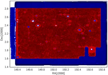
149:4 149:6 149:8 150:0 150:2 150:4 150:6 150:8 RA[J2000] 1:4 1:6 1:8 2:0 2:2 2:4 2:6 2:8 D ec [J 20 00 ]
Fig. 1.Distribution of the full COSMOS2015 (Laigle et al. 2016) source list over the COSMOS area (blue dots). The subset of 413 678 NUVrJ– based star-forming galaxies analysed in this work (red dots) includes sources fromLaigle et al.(2016) andMuzzin et al.(2013) within the UltraVISTA area, with the exception of masked regions due to saturated or contaminated photometry. See Sect.2for details.
22 38 (5.4%) are spectroscopically confirmed. The fraction of catastrophic failures (|zs− zp|> 0.15 × (1 + zs)) is only 3.4%.
Such a sizable sample enables us to bin galaxies as a func-tion of both M?and redshift, while maintaining good statistical
power. Figure2shows our sample in the M?–redshift diagram, highlighting the chosen grid. We note that the M?uncertainties taken from the parent catalogues incorporate the covariant errors on stellar population ages and dust reddening. These average M?
uncertainties are 0.2 dex at 108 < M
?/M < 109 and 0.1 dex
above, which is far smaller than the corresponding M? bin width, thus not impacting our results. The 90% M?
complete-ness limit (orange solid line, Laigle et al. 2016) indicates that our sample of SFGs is mostly complete down to 1010M
out to
z ∼4. Although we acknowledge the increasing incompleteness towards less massive galaxies in the early Universe, we believe that including them brings a valuable addition for constraining the infrared and radio properties of galaxies down to a poorly explored regime of M?. This will become particularly relevant
for the next generation of telescopes, such as JWST and SKA, which will routinely observe such faint sources. In addition, as we will discuss in Sect.3.3, a very good agreement is observed between our stacked LIR and those extrapolated from the MS
relation (Schreiber et al. 2015) also at M?< 109.5M ,
suggest-ing that even in this incomplete, low-M?regime our galaxies are still representative of an M?-selected sample. We emphasise that
the overall conclusions of this work remain unchanged when we limit ourselves to z < 3 and M?> 109.5M , where our sample is
largely complete. Moreover, in light of our main result, namely, that qIR decreases with M?, we anticipate that including
galax-ies within an incomplete M?regime would, at most, amplify the final M?dependence, thereby reinforcing our findings.
2.2. Infrared and sub-mm de-blended data
We complemented the existing COSMOS optical-to-IRAC pho-tometry with cutting-edge de-blended phopho-tometry fromJin et al.
(2018), which is based on the de-blending algorithm developed inLiu et al.(2018) for the GOODS-North field.
The dataset includes Spitzer-MIPS 24 µm data (PI: D. Sanders; Le Floc’h et al. 2009); Herschel imaging from the
PACS (100−160 µm,Poglitsch et al. 2010) and the SPIRE (250, 350, and 500 µm,Griffin et al. 2010) instruments, as part of the PEP (Lutz et al. 2011) and HerMES (Oliver et al. 2012) pro-grammes, respectively. In addition, JCMT/SCUBA2 (850 µm) images are taken from the S2CLS programme (Cowie et al.
2017;Geach et al. 2017), the ASTE/AzTEC (1.1 mm) data are
nested maps from Aretxaga et al. (2011) over a sub-area of 0.72 deg2. Finally,Jin et al.(2018) also included MAMBO data
(Bertoldi et al. 2007) at 1.2 mm over an area of 0.11 deg2. Briefly,Jin et al.(2018) used Ks-selected sources from the
UltraVISTA survey (Sect.2) as priors to perform a point square function (PSF) fitting of MIPS 24 µm, VLA-3 GHz (Smolˇci´c et al. 2017a), and VLA-1.4 GHz (Schinnerer et al. 2010) images down to the 3σ level in each band. Within our final sample, this procedure identifies 67 114 MIPS 24 µm+VLA priors. Never-theless, adopting a similar approach for extracting FIR/sub-mm flux densities of all M?-selected galaxies, that is, using the full list of Ks priors, would identify up to 50 sources per beam at
the resolution of the FIR/sub-mm wavelengths, leading to heavy confusion. Therefore, following Jin et al.(2018), only an M?
-complete subset of Ks priors was added, which ultimately
pri-oritises IR brighter sources. This leads to a total of 136 584 Ks+MIPS 24 µm+VLA priors, that were used to de-blend and
extract the Herschel, SCUBA2, and AzTEC flux densities (see Table1). Within our final sample of 413 678 star-forming galax-ies, 20 777 (5%) have a combined S /N > 3 over all FIR /sub-mm bands (10 285 at S /N > 5). These are displayed as red his-tograms in Fig.2. The rest of the Kssources are assumed to have
negligible FIR/sub-mm flux densities, consistent with the back-ground level in those bands. This is confirmed by the Gaussian-like behaviour of the noise (centered at zero) in the residual maps, after subtracting all S /N > 3 sources in each band (Jin et al. 2018). Throughout the rest of this paper, we interpret indi-vidual S /N > 3 sources as detections, while S /N < 3 sources will be stacked, as described in Sect.3.1.
2.3. Radio data in the COSMOS field
For our analysis, we exploited data from the VLA-COSMOS 3 GHz Large Project (Smolˇci´c et al. 2017a), one of the largest and deepest radio survey ever conducted over a medium sky area like COSMOS. With 384 h of observations, the final mosaic reaches a median root mean square (rms) of 2.3 µJy beam−1over 2.6 deg2 at an angular resolution of 0.7500, the highest among
radio surveys in COSMOS. A total of 10 830 sources were blindly extracted down to S /N > 5.
In addition, the COSMOS field boasts the current deepest radio-continuum data at 1.28 GHz from the MeerKAT Interna-tional GHz Tiered Extragalactic Exploration (MIGHTEE,Jarvis
et al. 2016) survey. With only 17 h of on-source observations
over the central 1 deg2of COSMOS, the early science release of
MIGHTEE reaches a thermal noise of 2.2 µJy beam−1, although the effective noise is limited by confusion. This provides an excellent sensitivity to large-scale radio emission. Neverthe-less, given the relatively large beam size (8.400× 6.800 FWHM),
MIGHTEE flux densities were de-blended using the same list of Ks+ MIPS 24 µm + VLA priors applied on FIR/sub-mm images
(Sect.2.2). Similarly, VLA radio flux densities were re-extracted based on the same PSF fitting technique down to S /N > 3. How-ever, for the sake of consistency with publicly available VLA catalogues, we take the 1.4 and 3 GHz radio flux densities of S/N > 5 sources fromSchinnerer et al.(2010) andSmolˇci´c et al.
(2017a), respectively. As a sanity check, we show in AppendixA
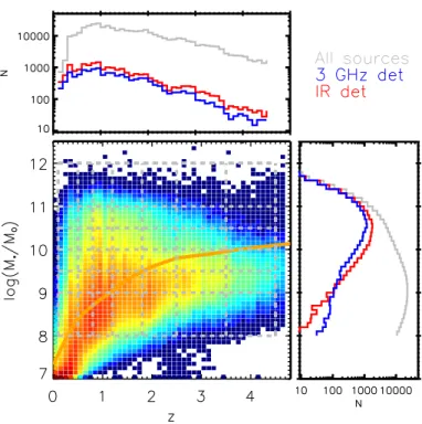
Fig. 2. Distribution of NUVrJ star-forming galaxies as a function of M? and redshift. The colour scale in the central panel indicates the underlying sample size, increasing from blue to red. The grey-dashed grid encloses the 42 M?−z bins into which we split our
sam-ple (413 678 objects). Galaxies within that grid are projected on the upper-leftand bottom right histograms with redshift and M?,
respec-tively (grey lines). The blue and red histograms represent the subsam-ple with a signal-to-noise ratio (S/N) that is greater than 3 at 3 GHz and across all IR bands, respectively (see Sects.2.2and2.3). The orange solid line marks the 90% M?completeness limit ofLaigle et al.(2016)
for comparison.
that our procedure leads to fully consistent total 3 GHz flux den-sities.
Given its unparalleled depth and resolution over the full COSMOS area, we primarily use the VLA 3 GHz dataset for our radio analysis, which counts 13 808 sources with S /N > 3 out of 413 678 M?-selected star-forming galaxies (∼3%). These radio detections are shown as blue histograms in Fig.2. Fainter sources will be accounted for via stacking, as described in Sect. 3.4. Nevertheless, repeating the same stacking analy-sis with ancillary radio datasets at 1.3 GHz (MIGHTEE) and 1.4 GHz (VLA) is essential to validating our procedure in the face of any potential variations of radio spectral index or di ffer-ent angular resolutions. We refer the reader to AppendixBfor an extensive comparison between stacking at 3 GHz and with ancil-lary radio datasets, whereas throughout this paper, we use radio data only at 3 GHz.
3. Stacking analysis
The aim of this paper is to investigate how the IRRC evolves with M? and redshift simultaneously. Contrary to studies in which galaxies were individually detected at IR or radio wavelengths, leading to complex selection functions and biased samples (see discussion inSargent et al. 2010), we start from a well-defined M?-selected sample. As a consequence, our analysis makes use of IR (Sect.3.1) and radio (Sect.3.4) stacking. This includes a careful treatment of some common caveats concerning IR galaxy samples, such as ‘clustering bias’ (Sect.3.2) and spectral energy distribution (SED) fitting including AGN templates (Sect.3.3).
Table 1. Main numbers of priors and detections that characterise our final sample of 413 678 star-forming galaxies.
Definition Number of sources
Final sample (this work) 413 678(∗∗)
– MIPS 24 µm+ VLA priors 67 114
– MIPS 24 µm+ VLA + Kspriors 136 584
– S /NIR> 3 20 777(∗∗)
– S /N3 GHz> 3 13 808(∗∗)
Notes. We note that subsets do not add up to make the final sample.
(∗∗)Numbers reported also in Fig.3.
8.0
9.0
9.5
10.0
10.5
11.0
12.0
log (M
*/ M
O •)
0.1
0.5
0.8
1.2
1.8
2.5
3.5
4.5
redshift
13494 0.6% 0.5% 3869 5.3% 3.4% 2408 29.1% 16.5% 1625 67.9% 39.9% 811 83.6% 54.7% 134 93.3% 56.0% 31233 0.2% 0.4% 9662 2.0% 1.2% 5597 10.4% 6.2% 3153 42.8% 25.3% 1499 64.3% 46.4% 220 73.2% 53.6% 47299 0.1% 0.4% 18521 1.4% 0.7% 11488 6.1% 3.0% 6260 28.5% 16.7% 2959 54.1% 37.8% 458 65.3% 60.5% 37632 0.1% 0.3% 22734 0.4% 0.6% 15912 4.5% 1.6% 9351 16.9% 9.2% 4592 38.0% 29.3% 838 47.9% 48.4% 28707 0.1% 0.4% 23777 0.2% 0.4% 14157 2.0% 1.1% 7088 10.8% 6.3% 3719 33.1% 24.8% 786 60.2% 52.5% 14187 0.2% 0.4% 21351 0.2% 0.4% 16035 1.0% 0.6% 7072 10.1% 3.7% 2389 30.3% 19.8% 456 63.2% 50.4% 4305 0.2% 0.3% 8398 0.4% 0.4% 6525 0.6% 0.7% 2289 7.8% 3.0% 520 29.2% 12.5% 168 56.5% 37.5%Fig. 3.Number of NUVrJ–based star-forming galaxies analysed in this work, as a function of M?and redshift (black). For convenience, in each bin we report the fraction of sources with combined S /NIR> 3 over all
FIR/sub-mm bands (red) and with S/N3 GHz> 3 (blue).
As for stacking radio data, special care is devoted to statistically removing radio AGN from our sample (Sect.4.2).
In addition, our notably large star-forming galaxy sample allows us to bin as a function of both M?and redshift, as shown in Fig.3. For each bin, we also report the total number of M?
-selected SFGs (black), as well as the corresponding fractions having combined S /NIR > 3 (red) and S/N3 GHz > 3 (blue).
As we can see, both fractions are a strong function of both M?
and redshift. Therefore, binning along both parameters enables us to account for the fact that galaxies of distinct M? are detectable at IR and radio wavelengths over different redshift ranges. These aspects will be extensively discussed when com-paring our results with previous literature (AppendixD). 3.1. Infrared and sub-mm stacking
In this section, we estimate the average flux densities across eight infrared and sub-mm bands, namely MIPS 24 µm, PACS 100−160 µm, SPIRE 250−350−500 µm, SCUBA 850 µm, and AzTEC 1100 µm. Similarly to other studies, we perform a median stacking on the residual maps fromJin et al.(2018), that is, after subtracting all detected sources with S /N > 3 in each band (see alsoMagnelli et al. 2009). Individual S /N > 3 detec-tions will be added to stacked flux densities a posteriori through a weighted average (Eq. (3)). Median stacking strongly mitigates contamination from bright neighbors and catastrophic outliers, and thus reduces the confusion noise for the faint sources. We
stress that our procedure yields very consistent results with either median or mean stacking of detections and non-detections com-bined (e.g.,Magnelli et al. 2015;Schreiber et al. 2015), as shown in Sect.3.3.
To produce stacked and rms images in each band, we used the publicly available IAS stacking library2 (Bavouzet et al. 2008;Béthermin et al. 2010). For each band, M? bin, and red-shift bin, we stack N × N pixel cutouts from the residual images, each centred on the NIR position of the M?-selected priors
(Sect.2). We chose the cutout size as eight times the full-width at half maximum (FWHM) of the PSF, while for Spitzer-MIPS, we chose 13 × FWHM, since a substantial fraction of the 24 µm flux is located in the first Airy ring. Since the AzTEC map covers only a central sub-area of 0.72 deg2, at 1.1 mm we only stacked
within that region. We emphasise that the M?, z, and SFR distri-bution of the SFG population within the AzTEC region is fully consistent with that derived in the rest of the COSMOS field, effectively not biasing the resulting stacked flux densities. To measure total flux densities, we followed different techniques depending on the input map. For MIPS and PACS images, we used a PSF fitting technique (e.g., Magnelli et al. 2014). A correction of 12% is further applied to account for flux losses from the high-pass-filtering processing of PACS images (e.g.,
Popesso et al. 2012;Magnelli et al. 2013). For SPIRE images, the photometric uncertainties are not dominated by instrumental noise but by the confusion noise caused by neighboring sources
(Dole et al. 2003; Nguyen et al. 2010). Since SPIRE images,
as well as those from SCUBA and AzTEC, are already bright-ness maps (in units of Jy beam−1 or equivalent), we read the
total flux from the peak brightness pixel. The total flux den-sity was taken as the median of the input cube at the central pixel.
The uncertainties on the stacked flux densities were mea-sured using a bootstrap technique (e.g.,Béthermin et al. 2015). Within each M?−z bin, we ran our stacking procedure 100 times, in all bands. For m non-detections at a given band, in each random realisation we re-shuffle the input sample, preserving the same total m by allowing source duplication. We take the median of the resulting flux distribution as our formal stacked flux. The 1σ dispersion around this value is interpreted as the flux error. We propagate this uncertainty in quadrature with the standard deviation of the stacked map across 100 random posi-tions within the cutout (after masking the central PSF). Although the latter component is typically sub-dominant relative to a boot-strapping dispersion, this conservative approach accounts for the strong fluctuations seen in low S/N stacked images, especially at low M?.
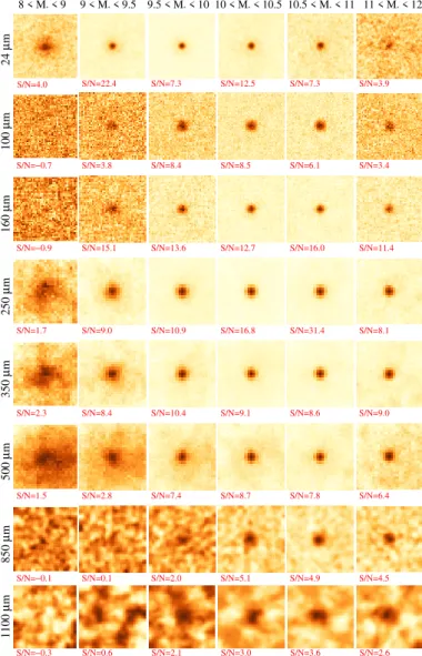
As an example, Fig.4shows stacked cutouts in all IR /sub-mm bands at 0.8 < z < 1.2 (i.e. close to the median redshift of our sample) as a function of M?. As expected from the tight MS
relation that links M?and SFR in star-forming galaxies, stacks at low M?display lower S/N, despite having larger numbers of
input sources.
3.2. Correcting for clustering bias
The stacked flux densities calculated above can be biased high if the input sources are strongly clustered or very faint. This bias is caused by the greater probability of finding a source close to another one in the stacked sample compared to a random position. This generates an additional signal, as has extensively 2 https://www.ias.u-psud.fr/irgalaxies/downloads.php
S/N=4.0 S/N=22.4 8 < M* < 9 9 < M* < 9.5 9.5 < M* < 10 10 < M* < 10.5 10.5 < M* < 11 11 < M* < 12 S/N=7.3 S/N=12.5 S/N=7.3 S/N=3.9 S/N=−0.7 100 µ m 24 µ m S/N=3.8 S/N=8.4 S/N=8.5 S/N=6.1 S/N=3.4 S/N=−0.9 160 µ m S/N=15.1 S/N=13.6 S/N=12.7 S/N=16.0 S/N=11.4 S/N=1.7 250 µ m S/N=9.0 S/N=10.9 S/N=16.8 S/N=31.4 S/N=8.1 S/N=2.3 350 µ m S/N=8.4 S/N=10.4 S/N=9.1 S/N=8.6 S/N=9.0 S/N=1.5 500 µ m S/N=2.8 S/N=7.4 S/N=8.7 S/N=7.8 S/N=6.4 S/N=−0.1 850 µ m S/N=0.1 S/N=2.0 S/N=5.1 S/N=4.9 S/N=4.5 S/N=−0.3 1100 µ m S/N=0.6 S/N=2.1 S/N=3.0 S/N=3.6 S/N=2.6
Fig. 4.Stacked cutouts of NUVrJ–based SFGs at 0.8 < z < 1.2, as a function of M?(left to right, expressed in log M ). Within each bin,
we stacked only those sources with S /N < 3 at a given band. SCUBA 850 µm and AzTEC 1100 µm images are smoothed with a Gaussian ker-nel to ease the visualisation. Each cutout size is 8 × FWHM of the PSF, while for Spitzer-MIPS, we chose 13 × FWHM. Below each cutout, we report the corresponding S/N.
been discussed in the literature (e.g., Bavouzet et al. 2008;
Béthermin et al. 2010,2012,2015;Kurczynski & Gawiser 2010;
Bourne et al. 2012; Viero et al. 2013; Schreiber et al. 2015). Given the large number of stacked sources in each bin, the S/N is typically good enough to be able to correct for this effect, which becomes more prominent with increasing beam size (e.g., up to 50% for SPIRE images, see Béthermin et al. 2015). Here, we briefly describe our approach, referring the reader to Appendix A.2 ofBéthermin et al.(2015) for a detailed explanation.
We model the signal from stacking as the sum of three com-ponents: a central point source with the median flux of the underlying population, a clustering component convolved with the PSF, and a residual background term (Eq. (2)). Following
Béthermin et al. (2015), we attempt to separate these
compo-nents via a simultaneous fit in the stacked images (Béthermin et al. 2012;Heinis et al. 2013,2014;Welikala et al. 2016). S(x, y)= ϕ × PSF(x, y) + ψ × (PSF ⊗ w)(x, y) + ε, (2)
Table 2. Average fraction of clustering signal at each FIR/sub-mm band.
Wavelength % Clustering signal
PACS 100 µm 11.3 ± 7.4 PACS 160 µm 10.2 ± 16.5 SPIRE 250 µm 25.9 ± 18.9 SPIRE 350 µm 31.3 ± 20.8 SPIRE 500 µm 42.7 ± 24.2 SCUBA 850 µm 19.2 ± 10.7 AzTEC 1100 µm 20.1 ± 12.9
Notes. Uncertainties indicate the 1σ dispersion among all S /N > 3 stacks at a given band.
where S (x, y) is the stacked image, PSF the point spread function, and w the auto-correlation function. The symbol ⊗ rep-resents the convolution. The parameters ϕ, ψ, and ε are free nor-malisations of the source flux, clustering signal, and background term, respectively.
We parametrise the ‘clustering bias’ as bias= ψ/(ϕ + ψ), once we have verified that residuals (i.e. ε) are always consistent with zero within the uncertainties. We do not see any obvious M?or redshift dependence of the clustering bias. However, at a
fixed wavelength, this can fluctuate significantly depending on the S/N of the input stacked image. For these reasons, we pre-fer to use an average clustering correction h1 − biasi for each band (see Table2), drawn only from stacks with S /N > 3. For those images, we multiply the stacked flux by h1 − biasi at the corresponding wavelength. Only the MIPS 24 µm data are not shown, since their flux densities are not used for SED fitting in Sect. 3.3. Uncertainties on the clustering corrections were propagated quadratically with the stacked flux errors obtained in Sect.3.1.
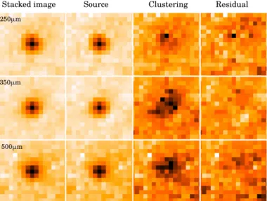
We stress that this method is suitable if the intrinsic source size is negligible compared to the PSF. This is especially true in SPIRE images, of which we show an example in Fig.5. This refers to a specific bin at 0.8 < z < 1.2 and 11 < log(M?/M ) <
12, for which all stacks give good enough S/N. Particularly for SPIRE images, the clustering bias can make up to 40% of the total flux, and it can be recognised as a more extended and dif-fuse emission. However, for consistency, we extend this analysis to the full set of FIR/sub-mm data.
Lastly, the clustering-corrected source flux densities (Sstack)
are combined with those of individual detections (Si) with
S/N > 3 in each band. If (m, n) is the number of stacked and detected sources, respectively, the weighted-average flux Sbinin
a given bin is derived as follows: Sbin=
m × Sstack+ Pni=1Si
n+ m · (3)
Flux uncertainties were propagated in quadrature. For stacks with S /N < 3 in which we could not constrain the clustering correction, Sstack was set to the noise level of the stacked map
(i.e. equal to its uncertainty). This way the weighted-average flux Sbinand its error are mainly driven by individual detections,
for which the flux could be measured more accurately (Jin et al. 2018). If the combined flux Sbinhas a S /N < 3, then it is set to
three times the noise and interpreted as a 3σ upper limit. 3.3. Conversion to LIRand SFR
This section illustrates how we fit the observed FIR /sub-mm SEDs to determine the total (8−1000 µm rest-frame) IR
Stacked image 250μmm
350μmm
500μmm
Source Clustering Residual
Fig. 5.Image decomposition of median stacks at 250, 350, and 500 µm, for a specific bin at 0.8 < z < 1.2 and 11 < log(M?/M ) < 12. From
left to right: the stacked image is separated among a point source PSF, the clustering signal, and a residual background term, respectively. The colour scale is normalised to the maximum in each cutout for visual purposes. See Sect.3.2for details.
luminosity within each M?−z bin. To this end, we use the two-component SED-fitting code developed byJin et al.(2018) (see also Liu et al. 2018). Briefly, this includes: three mid-infrared AGN torus templates fromMullaney et al.(2011); 15 dust con-tinuum emission models by Magdis et al. (2012) that were extracted fromDraine & Li(2007) to best reproduce the aver-age SEDs of MS (14) or SB (1) galaxies at various redshifts. While the Draine & Li(2007) models were based on a num-ber of physical parameters, the library ofMagdis et al. (2012) depends exclusively on the mean radiation field hUi= LIR per
unit dust mass (Md) and on whether the galaxy is on or above the
MS. However, on the MS the average dust temperature strongly evolves with redshift (e.g., Magnelli et al. 2014) and directly enters Md. Therefore, hUi and the SED shape both vary as a
function of redshift, for which Magdis et al. (2012) empiri-cally found as hUi ∝ (1+ z)1.15 up to z ∼ 2. More recently,
Béthermin et al.(2015) revised the evolution of hUi with red-shift out to z ∼ 4, using IR/sub-mm data in the COSMOS field, retrieving hUi ∝ (1+ z)1.8. Here, we adopt the set of 14 MS
templates fromMagdis et al.(2012), fit them to our data, and compare the hUi−z trend withBéthermin et al.(2015).
The SED-fitting routine performs a simultaneous fitting using AGN and dust emission models, looking for the best-fit solution via χ2 minimisation. In order to account for the
typi-cal photo-z uncertainty of the underlying galaxy population (at fixed M?,z), each template is fitted to the data across a range of ±0.05 × (1+ hzi) around the median redshift hzi. The code keeps track of each SED solution and corresponding normali-sation, generating likelihood distributions and uncertainties on for instance, LIR, hUi and AGN luminosity, if any. We note that
only FIR and sub-mm photometry (i.e. ignoring the MIPS 24 µm data-point) were used in the fitting procedure. This is done to avoid internal variations of the MIR dust features that cannot be captured by our limited set of templates (e.g., IR to rest-frame 8 µm ratio, IR8,Elbaz et al. 2011), which might affect the global FIR/sub-mm SED fitting. This optimisation clearly prioritises the FIR/sub-mm part of the SED, while not impacting the final LIRestimates (e.g.,Liu et al. 2018).
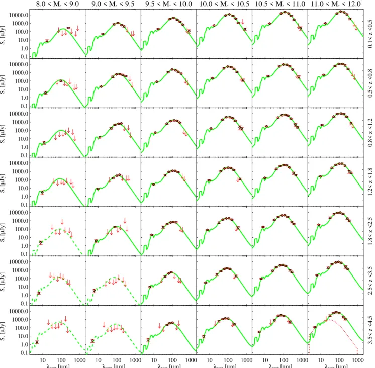
Figure 6 shows the best-fit star-forming galaxy template from theMagdis et al.(2012) library (green lines), as a function of M? (left to right, expressed in log M ) and redshift (top to
bottom). Red circles indicate the IR/sub-mm photometry, while downward arrows mark 3σ upper limits. The red dotted line is the best-fit AGN template fromMullaney et al.(2011), shown if significantly above 3σ. This is only found in the highest M?
and redshift bin. Green dashed lines represent SEDs without FIR measurements and at z & 1.5, for which the integrated LIR is
interpreted as 3σ upper limit (5/42 bins). Even though 24 µm has long been used as a proxy for LIR, this is only accurate at
z . 1.5 (e.g., Elbaz et al. 2011; Lutz 2014). For this reason we still interpret as measurements the LIR obtained from SEDs
without FIR data, but only at z . 1.5. That is the case for a few bins at the lowest M?, in which the SED reproduces a-posteriori the 24 µm data-point. Globally, our stacking analysis yields robust LIRestimates in 37/42 bins.
We find hUi ∝ (1+ z)1.74±0.18, which is fully consistent with
the revised hUi−z trend ofBéthermin et al.(2015): hUi ∝ (1+ z)1.8±0.4. This test is reassuring since it confirms that one single
z-dependent (or hUi–z-dependent) MS galaxy template is fully able to reproduce the observed SED across a wide M?interval.
Given the tight correlation between LIRand SFR, the IR data
have been extensively used as proxy for SFR, assuming that most of galaxy star formation is obscured by dust (Kennicutt 1998;
Kennicutt & Evans 2012). This is probably true inside the most massive star-forming galaxies (seeMadau & Dickinson 2014for a review). However, at decreasing M?, galaxies become more
metal-poor (e.g.,Mannucci et al. 2010) and, thus, less dusty and obscured. In these systems the ultraviolet (UV) domain provides a key complementary view on the unobscured star formation (Buat et al. 2012;Cucciati et al. 2012;Burgarella et al. 2013).
On this basis, the comprehensive work by Schreiber et al.
(2015) exploited IR-based SFRs (i.e. SFRIR) and
UV-uncorrected SFRs, in the deepest CANDELS fields, to cali-brate the star-forming MS over an unprecedented M? (down to M?= 109.5M ) and redshift range (z. 4). Since we carried out a
similar analysis, it is worth checking whether the SFR estimates based on our IR stacking reproduce or not the MS ofSchreiber et al.(2015).
For consistency, we need to collect the UV-uncorrected SFRs for our input sample. Hence, for each source we take the rest-frame NUV luminosity, LNUV (2800 Å), given in the
corre-sponding parent catalogue (Laigle et al. 2016orMuzzin et al. 2013) to estimate the UV-uncorrected SFR followingKennicutt
(1998): SFRUV[M yr−1]= 3.04 × 10⁻¹⁰L2800/L , already scaled
to aChabrier(2003) IMF. We verified that this conversion agrees well with more recent SFRUVprescriptions (e.g.,Hao et al. 2011; Murphy et al. 2011; see alsoKennicutt & Evans 2012).
Within each M?−z bin, we simply take the median SFRUV,
and we add it to the SFRIR corresponding to the stacked LIR,
calculated as SFRIR= 10−10LIR/L (Kennicutt 1998, scaled to
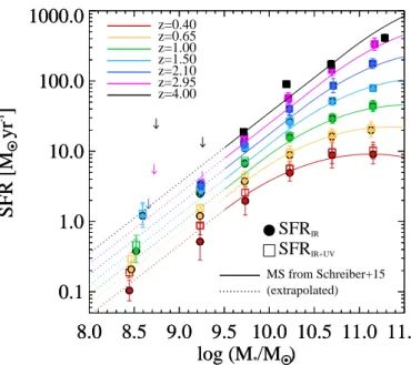
aChabrier 2003IMF). Figure7displays our data in the SFR–
M? plane, colour-coded by redshift over 0.1 < z < 4.5. At fixed M? and redshift, we show SFRIR (circles) and the total
SFRIR+UV(open squares) for comparison. Downward arrows are
3σ upper limits scaled from LIR. As can be seen, our data are
in excellent agreement with the evolving MS relation at all red-shifts (solid lines,Schreiber et al. 2015). While SFRUVappears
generally negligible compared to the total SFR, it becomes as high as SFRIRtowards low M?and low redshift (e.g.,Whitaker et al. 2012,2017). Our median values agree withSchreiber et al.
(2015), even below M? ∼ 109.5M , at which we extrapolate
8.0 < M* < 9.0 0.1 1.0 10.0 100.0 1000.0 10000.0 Sν [ µ Jy] 9.0 < M* < 9.5 9.5 < M* < 10.0 10.0 < M* < 10.5 10.5 < M* < 11.0 11.0 < M* < 12.0 0.1< z <0.5 0.1 1.0 10.0 100.0 1000.0 10000.0 Sν [ µ Jy] 0.5< z <0.8 0.1 1.0 10.0 100.0 1000.0 10000.0 Sν [ µ Jy] 0.8< z <1.2 0.1 1.0 10.0 100.0 1000.0 10000.0 Sν [ µ Jy] 1.2< z <1.8 0.1 1.0 10.0 100.0 1000.0 10000.0 Sν [ µ Jy] 1.8< z <2.5 0.1 1.0 10.0 100.0 1000.0 10000.0 Sν [ µ Jy] 2.5< z <3.5 10 100 1000 λREST [µm] 0.1 1.0 10.0 100.0 1000.0 10000.0 Sν [ µ Jy] 10 100 1000 λREST [µm] 10 100 1000 λREST [µm] 10 100 1000 λREST [µm] 10 100 1000 λREST [µm] 10 100 1000 λREST [µm] 3.5< z <4.5
Fig. 6.Best-fit template obtained from a SED-fitting decomposition (green lines), as a function of M?(left to right, expressed in log M ) and
redshift (top to bottom). Red circles indicate the IR/sub-mm photometry (MIPS 24 µm, PACS 100−160 µm, SPIRE 250−350−500 µm, SCUBA 850 µm, and AzTEC 1.1 mm), while downward arrows mark the corresponding 3σ upper limits. The red dotted line is the best-fit AGN template, shown in the only bin where its significance is above 3σ. Green dashed lines represent SEDs without FIR measurements and at z& 1.5, for which the integrated LIRis interpreted as 3σ upper limit (5/42 bins). MIPS 24 µm flux densities are not used in the fitting.
This test compellingly demonstrates that our LIRcan be deemed
robust over the full M? and redshift interval explored in this work.
3.4. Radio stacking at 3 GHz
In this section, we describe the equivalent stacking analysis done with radio 3 GHz (Smolˇci´c et al. 2017a) data, in order to derive average rest-frame 1.4 GHz spectral luminosities (L1.4 GHz) in
each M?−z bin. As is done for IR stacking (Sect.3.1), we treat detections and non-detections separately.
The total flux densities of radio sources with 3 < S /N < 5 were taken from Jin et al. (2018) (see Sect. 2.3), while for brighter sources we matched their flux densities to those of the corresponding catalogues. The purpose of this approach is twofold: using the same published flux densities for S /N > 5 detections for consistency and avoiding to deal with the effect of side-lobes from bright sources in stacked images, which might complicate total flux measurements (see Appendix A ofLeslie et al. 2020for a discussion). In addition, radio detections might contain a substantial fraction of AGN, which is expected to increase at higher M? (e.g.,Heckman & Best 2014). We will carefully deal with this issue in Sect.4.2. At relatively faint flux
8.0
8.5
9.0
9.5 10.0 10.5 11.0 11.5
log (M
*/M
O •)
0.1
1.0
10.0
100.0
1000.0
SFR [M
O •yr
-1]
8.0
8.5
9.0
9.5 10.0 10.5 11.0 11.5
log (M
*/M
O •)
0.1
1.0
10.0
100.0
1000.0
SFR [M
O •yr
-1]
SFR
IRSFR
IR+UV z=0.40 z=0.65 z=1.00 z=1.50 z=2.10 z=2.95 z=4.00 MS from Schreiber+15 (extrapolated)Fig. 7.SFR–M?relation of the NUVrJ star-forming galaxies selected in this work, colour-coded by redshift over 0.1 < z < 4.5. At fixed M?
and redshift, SFRIRmeasurements are converted from the LIRobtained
from IR/sub-mm SED-fitting (circles). Downward arrows indicate 3σ upper limits. For completeness, we also show the SFRIR+UVestimates by combining SFRIRwith UV-uncorrected SFRs (open squares). Solid
lines mark the evolving MS relation between SFRIR+UVand M?at di
ffer-ent redshifts (Schreiber et al. 2015). We observe an excellent agreement with the MS, even below M?∼ 109.5M that relies upon a linear
extrap-olation fromSchreiber et al.(2015) that is not constrained by previous data.
densities (<100 µJy), most of radio emission is thought to arise from star formation (Bonzini et al. 2015;Padovani et al. 2015;
Novak et al. 2017; Smolˇci´c et al. 2017a), though some
AGN-related radio emission might still be contributing (e.g., White et al. 2015;Jarvis et al. 2016). It is for this reason that median stacking of both detections and non-detections (e.g.,Karim et al.
2011; Magnelli et al. 2015) in deep VLA-COSMOS 1.4 GHz
images ought to result in minimal radio AGN contamination. This alternative approach will be tested in AppendixD.
Within the UltraVISTA area analysed in this work, the 3 GHz rms (2.3 µJy beam−1) fluctuates by less than 2% (Smolˇci´c et al. 2017b). Indeed, we anticipate that no difference between median or rms-weighted mean stacking of non-detections is observed (see AppendixAandLeslie et al. 2020), as detailed below. It is for these reasons that we chose to perform a median stacking of non-detections. Individual detections will be added a posteriori via a simple mean weighted average, as done in Eq. (3).
Our stacking routine generates cutouts with size of 8 × FW H M3 GHz (i.e. 600 at 3 GHz), centered on the NIR
posi-tion of each input galaxy. We acknowledge that an average o ff-set of 0.100 was found between 3 GHz (Smolˇci´c et al. 2017b) and UltraVISTA positions (Laigle et al. 2016), which is half the size of a pixel. To account for this systematic offset, our routine performs sub-pixel interpolation and searches for the peak flux (Speak) within ±1 pixel from the center of the stacked image. The
peak flux uncertainty is estimated via bootstrapping 100 times, as done in Sect.3.1. We take the median of the resulting flux distribution as our formal peak brightness. The 1σ dispersion around this value is interpreted as the corresponding error. We also measured the standard deviation across 100 random posi-tions in the stack (masking the central beam of 0.7500). This gives
less conservative errors compared to a bootstrap, but it is used to derive the formal rms of the stacked map.
Total flux densities (Stot) are calculated by fitting a 2D
ellip-tical Gaussian function to the median stacked image, using the IDL routine
mpfit
2dfun
3. Given the typically high S/N (∼10 on average) reached in the central pixel, we leave size, position angle, and normalisation of the 2D Gaussian as free parameters. We verified that adopting a circular Gaussian or forcing the nor-malisation to the peak flux does not significantly affect any of our stacks. The total flux was calculated by integrating over the 2D Gaussian area Agauss. The integrated flux error was computed bymultiplying the peak flux error by pAgauss/Abeam, where Abeam
is the known beam area, and adding a known 5% flux calibra-tion error in quadrature (Smolˇci´c et al. 2017a). We recall that the peak flux error already incorporates the variance of the stacked sample via bootstrapping.
In order to assess whether our sources are clearly resolved, we follow the same criterion applied to VLA 3 GHz detections (Smolˇci´c et al. 2017a) to identify resolved sources:
Stot
Speak
> 1 + (6 × S/Npeak)−1.44, (4)
where S /Npeak is simply the peak flux divided by the rms of
the image. This expression was obtained empirically to define an envelope containing 95% of unresolved sources, below such threshold. We find that 31 stacks out of 42 are resolved, accord-ing to Eq. (4). For these, total flux densities are on average 1.8× higher than peak flux densities. Similarly, Bondi et al. (2018) found 77% of VLA 3 GHz detected SFGs are resolved, and this fraction does not change significantly with M? ( Jiménez-Andrade et al. 2019). Of the 11 bins with unresolved emission, 3 have S /Npeak < 3; these are all among the 5 bins without LIR
estimates from IR stacking (Sect.3.3). Analogously to our treat-ment of the IR measuretreat-ments, we discard all those 5 bins from the rest of our analysis.
For the stacks with resolved emission, we prefer to use their integrated flux from 2D Gaussian fitting as the most accurate estimate. Instead, for unresolved stacks we use the peak flux, consistent with the treatment of 3 GHz detections (Smolˇci´c et al. 2017a). Fitting residuals are on average 3% of the total flux and always consistent with zero within the uncertainties. We validate this approach by reproducing the total flux densities of 3 GHz detections presented inSmolˇci´c et al.(2017a) at S /N > 5 and in
Jin et al.(2018) at 3 < S /N < 5, respectively (AppendixA). Finally, we combined the radio stacked flux densities within each M?−z bin together with individual detections,
follow-ing Eq. (3). The combined 3 GHz flux densities were first scaled to 1.4 GHz assuming of Sν ∝ να, with spectral index
α = −0.75 ± 0.1 (e.g.,Condon 1992;Ibar et al. 2009,2010). This assumption is discussed in Appendix B. Lastly, 1.4 GHz flux densities were converted to rest-frame 1.4 GHz spectral lumi-nosities (L1.4 GHz), again assuming α= −0.75. Formal L1.4 GHz
errors were calculated by propagating the uncertainties on both combined flux and spectral index.
The various checks described in Appendix B prove our
L1.4 GHzrobust across the full range of M?and redshift analyzed
in this work. We note that our L1.4 GHzestimates do not
necessar-ily trace radio emission from star formation. Indeed, radio AGN are not yet removed at this stage, and they might be potentially boosting the L1.4 GHz. This issue is addressed in Sect.4.2. 3 https://pages.physics.wisc.edu/~craigm/idl/fitqa.
4. The IRRC and the contribution of radio AGN Using the median LIR and L1.4 GHz obtained from stacking, we
study the evolution of the IRRC as a function of M?and redshift.
Logarithmic uncertainties on each luminosity were propagated quadratically to get qIR errors. Among the 42 M?−z bins
ana-lyzed in this work, 37 yield robust estimates of LIR and L1.4 GHz,
while the remainder are discarded from the following analysis. Unsurprisingly, these latter 5 bins (three at 108< M
?/M < 109
and 1.8 < z < 4.5; two at 109< M?/M < 109.5and 2.5 < z < 4.5)
are among the least complete in M?, as highlighted in Figs.2
and6. Therefore their exclusion partly mitigates the M? incom-pleteness of the remaining sample.
4.1. qIRbefore removing radio AGN
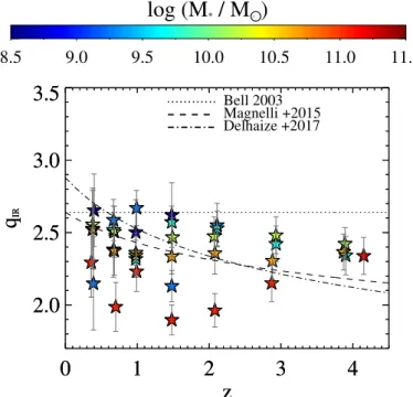
Figure 8 shows the average qIR as a function of redshift,
colour-coded in M? (stars). For comparison, other prescrip-tions of the evolution of the IRRC are overplotted (black lines).
Bell (2003) inferred the average IRRC in local SFGs, find-ing qIR= 2.64 ± 0.02 (dotted line), with a scatter of 0.26 dex. Magnelli et al. (2015) studied an M?-selected sample at z .
2, and constrained the evolution of the far-infrared radio cor-relation (FIRC, parametrised via qFIR4) across the SFR–M?
plane at M? > 1010M . From stacking IR and radio images,
they parametrised the evolution with redshift of the FIRC as: qFIR= (2.35 ± 0.08) × (1 + z)−0.12±0.04, where the normalisation
is scaled to 2.63 in the qIR space. More recently, Delhaize et al. (2017) exploited a jointly-selected sample of IR (from Herschel PACS/SPIRE) or radio (from the VLA-COSMOS 3 GHz Large Project,Smolˇci´c et al. 2017a) detected sources (at ≥5σ) in the COSMOS field. Through a survival analysis that accounts for non-detections in either IR or radio, they inferred the evolution of the IRRC with redshift out to z ∼ 4 as: qIR= (2.88 ± 0.03) × (1 + z)−0.19±0.01. While this trend appears
somewhat steeper than that ofMagnelli et al. (2015), we note thatDelhaize et al.(2017) did not formally remove objects with significant radio excess, whileMagnelli et al.(2015) performed median radio stacking to mitigate the impact of potential outliers such as radio AGN. Nevertheless, Delhaize et al.(2017) argue that the IRRC trend with redshift would flatten if applying a 3σ-clipping: qIR= (2.83 ± 0.02) × (1 + z)−0.15±0.01, which becomes
fully consistent with the findings ofMagnelli et al.(2015). When compared to the above literature, it is evident that our qIR values lie systematically below other studies at M? >
1011M , while lower M? galaxies lie closer or slightly above
them. In other words, our qIR estimates seem to display a clear
M? stratification, with the most massive galaxies having typi-cally lower qIR than less massive counterparts. As mentioned
earlier in this work, we recall that our sample, at this point, contains some fraction of radio AGN, which might be boosting the L1.4 GHz, particularly at high M?(see e.g.,Best & Heckman 2012) where radio AGN feedback is known to be prevalent. Our LIRestimates are, instead, corrected for a potential IR-AGN
con-tribution (Sect.3.3). Therefore, the net effect caused by includ-ing AGN is lowerinclud-ing the intrinsic qIR. Selecting typical SFGs on
the MS is expected to, however, reduce the incidence of power-ful radio AGN expected in massive hosts since most radio AGN at z < 1 are found to reside in quiescent galaxies (e.g.,Hickox et al. 2009; Goulding et al. 2014). It is for these reasons that we caution that Fig.8should be taken as the AGN-uncorrected 4 The far-infrared luminosity used to compute q
FIR was integrated
between 42 and 122 µm rest-frame. This is quantified to be 1.91× smaller than the total LIR(Magnelli et al. 2015).
0
1
2
3
4
z
2.0
2.5
3.0
3.5
q
IR0
1
2
3
4
z
2.0
2.5
3.0
3.5
q
IR Bell 2003 Magnelli +2015 Delhaize +2017log (M
*/ M
O ·)
8.5
9.0
9.5
10.0
10.5
11.0
11.5
Fig. 8.AGN-uncorrected qIRevolution as a function of redshift (x-axis)
and M?(colour bar). Errors on qIRrepresent the 1σ scatter around the
median value, estimated via bootstrapping over LIR and L1.4 GHz. For
comparison, other IRRC trends with redshift are taken from the liter-ature (black lines):Bell(2003, dotted);Magnelli et al.(2015, dashed); Delhaize et al.(2017, dot-dashed). Our qIRvalues still include the
con-tribution of radio AGN. See Sect.4.1for details.
qIR. However, it is worth showing it to quantify how much qIR
changes after removing the radio AGN. 4.2. Searching for radio AGN candidates
In this section, we describe how we carried out a detailed study aimed at identifying potential radio AGN, removing them, and ultimately deriving the intrinsic qIR trend that is purely driven
by star formation. In our radio analysis, we combined individ-ual radio-detections (above S /N > 3) with undetected sources via a weighted average (Eq. (3)). Contrary to stacking detections and non-detections together, this formalism enables us to char-acterise the nature of individual radio detections, that is, whether they show excess radio emission relative to star formation.
We accept an underlying assumption that radio-undetected AGN do not significantly affect any of our radio stacks. This is supported by the excellent agreement between mean- and median-stacked L1.4 GHz of non-detections (Fig. A.2, bottom
panel). Indeed, if the contribution of radio-undetected AGN were substantial, the corresponding mean L1.4 GHzwould be
sig-nificantly higher than the median L1.4 GHz from stacking. This
assumption is further supported by the fact that the fraction of identified radio AGN is a strong function of radio flux den-sity, and the sources we stack are, by construction, faint in the radio.Algera et al.(2020c) argue that below 20 µJy (at 3 GHz), the fraction of radio-excess AGN is <10% (see also Smolˇci´c
et al. 2017b; Novak et al. 2018). We acknowledge that our
assumption does not allow us to collect a complete sample of radio AGN, especially at high redshift where the fraction of radio detections notably drops (Fig. 3). Nevertheless, we will show that any residual AGN contribution does not change our conclusions.
1
2
3
4
q
IR8.0<log(M
*/M
O •)<9.0
3GHz det: 510 (3.5% IR det) stacks undet (stacks undet) + det
L
IR/ L
1.4, LIM9.0<log(M
*/M
O •)<9.5
3GHz det: 605 (17.5% IR det)9.5<log(M
*/M
O •)<10.0
3GHz det: 1636 (43.8% IR det)0
1
2
3
4
z
1
2
3
4
q
IR10.0<log(M
*/M
O •)<10.5
3GHz det: 4162 (68.8% IR det) qIR peak #1 complete z-bin0
1
2
3
4
z
10.5<log(M
*/M
O •)<11.0
3GHz det: 5045 (76.3% IR det)qIR peak best-fit with z #5 complete z-bins
0
1
2
3
4
z
11.0<log(M
*/M
O •)<12.0
3GHz det: 1552 (78.3% IR det)qIR peak best-fit with z #7 complete z-bins
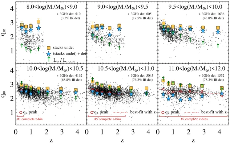
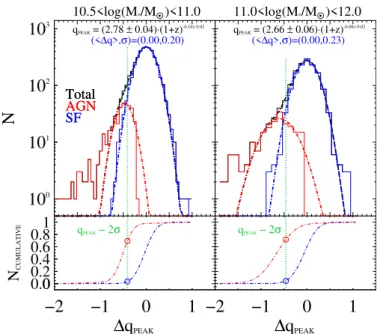
Fig. 9.Distribution of qIRas a function of redshift, split across increasing M?bins. In each panel, we compare the qIRestimates of individual radio
detections (black dots) with the median stacked values of non-detections (yellow squares) and with the weighted-average qIRof detections and
non-detections together (from Eq. (3), blue stars). Green upward arrows indicate the corresponding threshold qIR,limabove which radio detections
become inaccessible from an M?-selected sample. We select relatively complete M?−z bins, in which at least 70% of radio detections have qIR
below the corresponding threshold. This criterion identifies 13 bins (in red square brackets). Within these bins, the peak of qIRdistribution (qIR,peak)
is indicated with red open circles. In the two highest M?bins, the best fitting trends with redshift are shown by the red dashed lines. Each panel
reports the number of individual 3 GHz sources and their fraction with S /NIR> 3. See Sect.4.2.1for details.
We briefly summarise our next steps as follows. In Sect.4.2.1, we explore the qIRdistribution traced by individual
3 GHz detections as a function of M?and redshift. First, we iden-tify a subset of radio detections at M? > 1010.5M that is
rep-resentative of an M?-selected sample. Then we decompose their qIR distribution between AGN and star formation components
(Sect. 4.2.2). This enables us to subtract potential radio AGN candidates and to calibrate the intrinsic best-fit IRRC with red-shift at M? > 1010.5M (Sect.4.2.3). Then we extrapolate this
calibration towards lower M?bins (Sect.4.2.4), where a similar in-depth analysis was not possible due to radio-detections being strongly incomplete in this M?regime. Finally, the intrinsic (i.e. AGN-corrected) IRRC as a function of M? and redshift is pre-sented in Sect.4.3.
4.2.1. The qIRdistribution of radio detections
In order to study the qIR distribution of 3 GHz detections, we
need to calculate their average LIR as a function of M?and
red-shift. For convenience, we refer the reader back to Fig.2(blue histograms) for visualizing the distribution of 3 GHz detections in the M?−z space. Out of 13 510 radio detections among our 37 bins, 8762 (65%) have a combined S /NIR > 3, therefore
reliable LIRmeasurements from SED-fitting of FIR/sub-mm
de-blended photometry (Jin et al. 2018). For the remainder of the sample, we stack again their IR/sub-mm images in all bands in
each M?−z bin. Stacked IR flux densities are corrected for clus-tering bias and converted to LIR following the same procedure
adopted for the prior M? sample (Sect. 3.1). Median stacked LIRare retrieved for the same 37/42 bins of the full parent
sam-ple, since a stacked S /N > 3 flux was obtained in at least one FIR/sub-mm band. Then, for each source we re-scaled its median stacked LIRto the redshift and M?of that source (assuming the
MS relation), in order to reduce the variance of the underlying sample within each M?−z bin. We verified that our stacked LIR
are always systematically below the 3σ LIRupper limits inferred
from FIR/sub-mm SED-fitting (Jin et al. 2018). This ensures that our stacking analysis provides more stringent constraints on the LIRof individual non-detections.
From this analysis, we are well-placed to explore the full qIR
distribution of 3 GHz detections at different M? and redshifts. Figure 9 shows qIR as a function of redshift, split in six M?
bins. Black dots mark individual 3 GHz detections, blue stars represent the qIR obtained by combining detections and
non-detections (same as in Fig. 8), while yellow squares are the stacks of non-detections only. In each panel we report the num-ber of 3 GHz detected sources and the fraction of them with com-bined S /NIR> 3. This fraction strongly increases with M?, from
3.5% at 108< M
?/M < 109to 78.3% at 1011 < M?/M < 1012,
which implies that at the lowest M? nearly all qIR estimates of
radio detections rely upon IR stacking. This is because the 3 GHz detection limit sets a rough threshold in SFR (if radio emis-sion primarily arises from star formation), therefore, it is biased