HAL Id: insu-00615428
https://hal-insu.archives-ouvertes.fr/insu-00615428
Submitted on 11 Oct 2011HAL is a multi-disciplinary open access archive for the deposit and dissemination of sci-entific research documents, whether they are pub-lished or not. The documents may come from teaching and research institutions in France or abroad, or from public or private research centers.
L’archive ouverte pluridisciplinaire HAL, est destinée au dépôt et à la diffusion de documents scientifiques de niveau recherche, publiés ou non, émanant des établissements d’enseignement et de recherche français ou étrangers, des laboratoires publics ou privés.
Singular value decomposition as a denoising tool for
airborne time domain electromagnetic data
Pierre-Alexandre Reninger, Guillaume Martelet, Jacques Deparis, José Perrin,
Yan Chen
To cite this version:
Pierre-Alexandre Reninger, Guillaume Martelet, Jacques Deparis, José Perrin, Yan Chen. Singular value decomposition as a denoising tool for airborne time domain electromagnetic data. Journal of Applied Geophysics, Elsevier, 2011, 75 (2), pp.264-276. �10.1016/j.jappgeo.2011.06.034�. �insu-00615428�
Singular value decomposition as a denoising tool for airborne time
domain electromagnetic data
P.-A. Reningera, b,, G. Marteleta, J. Deparisa, J. Perrina, Y. Chenb
aBureau de Recherches Géologiques et Minières (BRGM), GEO/G2R, 3, Avenue Claude
Guillemin, 45060 Orléans Cedex 2, France
b Institut des Sciences de la Terre d'Orléans (ISTO), Université d'Orléans, UMR 6113, 1A,
rue de la Férollerie, 45071 Orléans Cedex 2, France
Abstract
Airborne time domain electromagnetic (TDEM) surveys are increasingly carried out in anthropized areas as part of environmental studies. In such areas, noise arises mainly from either natural sources, such as spherics, or cultural sources, such as couplings with man-made installations. This results in various distortions on the measured decays, which make the EM noise spectrum complex and may lead to erroneous inversion and subsequent
misinterpretations. Thresholding and stacking standard techniques, commonly used to filter TDEM data, are less efficient in such environment, requiring a time-consuming and
subjective manual editing. The aim of this study was therefore to propose an alternative fast and efficient user-assisted filtering approach. This was achieved using the singular value decomposition (SVD). The SVD method uses the principal component analysis to extract into components the dominant shapes from a series of raw input curves. EM decays can then be reconstructed with particular components only. To do so, we had to adapt and implement the SVD, firstly, to separate clearly and so identify easily the components containing the
geological signal, and then to denoise properly TDEM data.
The reconstructed decays were used to detect noisy gates on their corresponding measured decays. This denoising step allowed rejecting efficiently mainly spikes and oscillations. Then, we focused on couplings with man-made installations, which may result in artifacts on the inverted models. An analysis of the map of weights of the selected ―noisy components‖ highlighted high correlations with man-made installations localized by the flight video. We had therefore a tool to cull most likely decays biased by capacitive coupling noises. Finally, rejection of decays affected by galvanic coupling noises was also possible locating them through the analysis of specific SVD components. This SVD procedure was applied on airborne TDEM data surveyed by SkyTEM Aps. over an anthropized area, on behalf of the French geological survey (BRGM), near Courtenay in Région Centre, France. The established denoising procedure provides accurate denoising tools and makes, at least, the manual
cleaning less time consuming and less subjective.
Keywords: Time domain electromagnetism (TDEM); Transient electromagnetism (TEM); Singular value decomposition (SVD); Denoising; Filter; Airborne
1. Introduction
Electromagnetic (EM) methods were historically developed for mining purposes (see Palacky and West, 1991 for a review). The ability of time domain electromagnetism (TDEM) method to provide increasingly detailed resistivity mapping of the underground progressively makes
the method suitable in environmental studies (Jørgensen et al., 2003). For these applications, high accuracy of the measured data is needed (Sørensen and Auken, 2004).
A mathematical description of EM in geophysics is given by Ward and Hohmann (1988). The signal-to-noise ratio of a typical measured sounding is good at early times and signal is overwhelmed by the background noise at late delay times (Munkholm and Auken, 1996). However, the measured decay may also be affected by high amplitude noises when surveying. The EM noise spectrum has been studied by many authors as [Macnae et al., 1984] ,
[McCracken et al., 1984] , [McCracken et al., 1986] and [Spies and Frischknecht, 1991] . The spectrum is colored (Munkholm and Auken, 1996) and has diurnal, annual and geographical variations. Spherics, arising from thunderstorms, and Very Low Frequency (VLF)/Amplitude Modulated (AM) transmitters, around 15 kHz–24 kHz and 200 kHz respectively, may
dominate the measured magnetic field ( [Effersø et al., 1999] and [Spies and Frischknecht, 1991] ). Induced polarization (IP) effects may also occur with a sufficiently polarizable earth (Flis et al., 1989) and results mainly in a noticeable sign reversal at late delay times in coincident-loop configuration.
An accurate measurement is therefore not sufficient and a processing is often required in order to obtain a better and more realistic resistivity model after the inversion. As part of TDEM processing, several attempts were made to filter noise in decays ( [Bouchedda et al., 2010] , [Buselli and Cameron, 1996] , [Macnae et al., 1984] and [Palacky and West, 1991] ). Existing filters may remove/reduce spikes or oscillations on decays. Noise reduction allows improving the penetration depth of the signal without having to increase the transmitter power or acquisition time (Spies, 1988). Prediction filters/recursive algorithms ( [Buselli et al., 1998] , [Buselli and Cameron, 1996] and [Spies, 1988] ) can be used to filter TDEM data but they require many input parameters. Other filters have been developed for ground measurements and are only optimized for small surveys (Stephan and Strack, 1991). More recently,
Bouchedda et al. (2010) used two techniques which operate in the wavelet domain for the spherics noise reduction. However, these filters are very specific to an acquisition setup and/or target a single source of noise.
Nowadays, the most common general denoising methods use threshold and/or stacking ( [Cull, 1991] , [HGG, 2011] , [Macnae et al., 1984] and [McCracken et al., 1984] ). Thresholding can be applied either on pre-stacked data ( [Macnae et al., 1984] and
[McCracken et al., 1984] ), in order to improve the signal-to-noise ratio when stacking, or on stacked data (HGG, 2011), in order to reject the noise from the decays. Stacking and
thresholding methods are efficient to remove/reduce mainly noises such as spherics and background noises. However, surveys are increasingly carried out in anthropized areas ( [Auken et al., 2009] and [Viezzoli et al., 2010] ) where other noise sources may be
superimposed ( [Junge, 1996] and [Szarka, 1988] ). Noises, in anthropized areas, arise mainly from the power distribution grid (50/60 Hz) but the measured responses can also locally be distorted by couplings with man-made installations ( [Danielsen et al., 2003] and [Sørensen et al., 2000] ) such as power lines, metallic pipes and insulated underground cables. These coupling noises can be either capacitive or galvanic. Capacitive coupling may distort the time constant at early times and results in oscillations in the data, making it easy to recognize. Galvanic coupling results in a time constant distortion of the measured decay (Nekut and Eaton, 1990) and is difficult to distinguish since the decay looks like a normal TDEM sounding which would have been measured above a geological conductive structure.
Moreover, coupling noises can also result in an amplitude shift of the decay curve. This can only be recognized thanks to the neighboring soundings; this is difficult on airborne EM data
because of the changes in altitude, which produce somehow equivalent effects. In detail, the effects of these two couplings depend mainly on the size and the shape of the man-made installation, as well as its distance and orientation to the receiver (Danielsen et al., 2003). In an anthropized area, noise is complex and not predictable. The stacking is therefore less efficient and threshold filtering does not consistently and adequately remove noise. Thus, a manual cleaning is generally needed, which makes the filtering very time-consuming and subjective.
The aim of our work was therefore to suggest an efficient general denoising tool for raw stacked TDEM data, provided by airborne survey companies. This was achieved adapting the singular value decomposition (SVD) to TDEM data. The SVD method is a standard
processing tool for gamma-ray data since the late nineties (Hovgaard and Grasty, 1997). An approach of the same kind using Principal Component Analysis (PCA) has already been applied on EM data (Green, 1998) but not as a general denoising method. Here we develop an original approach using the SVD statistical analysis of the dataset to map noise and filter/edit its effects on the data.
2. SkyTEM data
The GeoCentre project focuses on geo-environmental objectives such as geological and hydrogeological issues in Region Centre, France. For this purpose, airborne TDEM
measurements were carried out by SkyTEM ApS. from February to March 2009. The survey requested by BRGM (French geological survey) consisted of three separated zones:
Courtenay, Vierzon and Sud-Cher. The survey, flown with 400 m line spacing over a total of about 978 km², represents about 3000 km of flight lines. The spacing between each EM sounding along flight lines was around 30 m.
The SkyTEM is a helicopter-borne TDEM system ( [Auken et al., 2007] and [Sørensen and Auken, 2004] ) developed for hydrogeophysical and environmental investigations by the Hydro Geophysics Group (HGG) at the University of Aarhus, Denmark. The SkyTEM system is capable of operating in a dual transmitter mode. The Low Moment provides early time data for shallow imaging, whereas, the High Moment allows measuring later time data for deeper imaging.
During the measurements, the system integrates several steps of signal processing in order to reduce noise. First, the signal-to-noise ratio is improved using log-gating and gate stacking techniques (Munkholm and Auken, 1996). The term log-gating refers to the integration of the input signal on logarithmic gate widths (time interval) in order to keep a dense sampling at early times and increase the signal-to-noise ratio with longer averaging intervals at later delay times, as the background noise increases. The average value during each time interval is then assigned to the center of each time gate and is considered as the measured amplitude of the secondary field. The gate stacking refers to the stack of values of several measured decays at the same delay time. Strack et al. (1989) have suggested deleting incoherent measurements by ordering data by amplitude before stacking. Secondly, the spectral peak at 50/60 Hz due to the power distribution grid is rejected thanks to the polarity changes of the transmitter wave and its base frequency (harmonic of 50/60 Hz). Finally, AM and VLF transmitters noises are rejected using TDEM receivers measuring in segments, where each segment is band-limited by Low Pass filters; their bandwidth is broad at early times and narrow at late times (Effersø et al., 1999).
TDEM data used in this study are those provided by SkyTEM ApS. They had already been stacked and we considered that the background, the power distribution grid and the AM and VLF transmitter noises had been reduced. However, it still remained distortions in the data, coming mainly from the coupling noises and the spherics, on which our filtering was focused. The vertical component of the secondary field only was studied.
3. The singular value decomposition (SVD) and its applications
3.1. SVD Theory
The SVD uses orthogonal components to extract the dominant shapes from a series of raw input curves (i.e. decays). It is a multivariate analysis approach. The SVD method analyzes the dispersion around the origin through the decomposition of the signal into a series of principal components (Press et al., 1992).
The principal components (PC) of a set of n curves put in a matrix A are the eigenvectors of the covariance matrix ATA. They are mutually orthogonal and sorted, by eigenvalues, into descending order. The first principal component is the single shape which explains most of the curve variance (i.e. the average) while the second principal component explains most of the curve variance not explained by the first principal component (i.e. the average of the residual), and so on for subsequent components.
The principle of the method is to extract desired signal from the data by reconstructing the curves considering specific components. If curves are affected by a normally distributed noise with equal variance and zero mean, the lower-order components explain the geological part of the signal and higher-order components represent noise. The SVD method is based on the following theorem (Press et al., 1992). Any m × n matrix A (m ≥ n) can be written as the product of 3 matrices:
A=UWVT
Where U is m × n, VT is n × n and W is an n × n diagonal matrix. V is orthogonal and the columns of U are orthonormal. The principal components are the columns of V, and the eigenvalues are the square of the elements of W. U is the matrix of the weights of each component at each measurement location and V is the matrix of the uncorrelated shapes. Thus, for a dataset of m curves of n gates, the application of the SVD method results in n uncorrelated shapes.
3.2. Adapting SVD to TDEM data
SVD is commonly used in processing of gamma-ray spectrometry data. In gamma-ray spectrometry, the variance associated with each channel for each spectrum is not equal. The low-energy channels (Compton effect) have count rates up to 150 times larger than the high-energy channels. This means that low-high-energy channels completely dominate the PC analysis. Hovgaard (1997), based on the fact that the data matrix is a Poisson realization, suggested to scale each observed spectrum by the best fit of the average spectrum; it is the Noise
Adjustment of the SVD (so-called NASVD). In gamma-ray data processing, the 3–6 first components generally explain entirely the uranium, potassium and thorium variables whereas the higher order components correspond to the noise.
The problem for EM data is different, because the physics and the measurement principle are different. Measured TDEM decays are amplitudes in function of time instead of photon counting in function of energy. Moreover, the influence of the geology and altitude of the receiver induce important variations of shape and dynamics from one decay to another. Therefore, the scaling of the data as implemented by Hovgaard (1997) is inadequate for EM data. The scaling by the logarithm was tried but didn't work since noise mostly occurring at late delay times was amplified. The solution used to reduce the dynamics of the curves (i.e. the variance) and therefore to rescale noises around a common level was to multiply each decay gate by its gate width (time interval of integration). However, given the complexity of the EM noise spectrum, the separation between the noise and the geological part of the signal is not as straightforward as in gamma-ray spectrometry.
In order to improve the separation power of the SVD and to simplify the understanding of the components, the SVD was run on the absolute values of each gate (see details in Section 4. Discussion–conclusion).
The denoising process was performed as follows. First, a SVD was run to decompose the measured decays into components. Then, we characterized the components in order to identify which ones should not be kept to reconstruct the decays. Finally, we used the components to map and characterize the noise on the study area.
3.3. Implementation of the SVD method: pre-denoising step
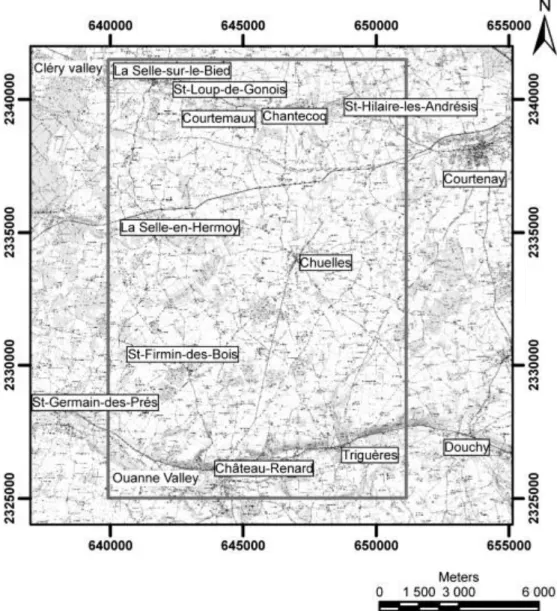
In the following, the SVD filtering method is illustrated on the dataset surveyed near Courtenay, France. The survey was flown over an anthropized area (Fig. 1). To avoid
redundancy, processing of Low Moment is not reported; only the results on the High Moment data (22 gates per decay) will be shown and discussed here. The Courtenay survey includes about 540 km of flight lines, which represent 12 000 soundings. Thus, we had enough data to perform significant statistics on this dataset. First, we interpreted the components which we then mapped.
The components are sorted into descending amplitudes. The order of each component is strongly influenced by its contribution in terms of variance during the SVD reconstruction. Given the principle of the SVD (i.e. each component being the average of the previous residual), the first components vary more smoothly than the following. Indeed, we explain, first, components accounting for the general trend of the decays and then components
accounting for more subtle variations, while increasing the order of the component. Therefore, oscillations and spikes induced by noise are rather explained by the high order components and can be separated from the geological signal. Thus, in the following, components displaying patterns corresponding to regular decays will be referred as ―geological
components‖ and those displaying patterns corresponding to spikes and oscillations coming from spherics, capacitive coupling and background noises will be referred as ―noisy
components‖.
The aim is therefore to keep the ―geological components‖ to reconstruct the decays. However, on the standard representation of components in Fig. 2, the separation between geological noisy components may be unclear.
Another representation of the components is therefore proposed: rather than the components themselves, we plotted the variations introduced by each component with respect to the
average decay (i.e. the first component; see Fig. 3 and Appendix A); amplitudes of the
components have been weighted by their eigenvalues. With this new representation, typically, a ―noisy component‖ is characterized by oscillations around the mean, i.e. the two curves coincide except at gates where spikes occur in the considered component (Fig. 3b, d). Instead, a ―geological component‖ introduces a different pattern from that explained by the first component on part or all of the decay, so that the two curves have two different trends (Fig. 3a, c). Compared to Fig. 2 and Fig. 3 actually simplifies the identification of the ―noisy components‖. It must be noted that oscillations around the mean induced by the ―noisy components‖ are amplified when multiplying with the weight matrix U.
Based on this analysis, component by component, of plots such as displayed in Fig. 3, the components 1, 2, 3, 4, 5, 6 and 8 have been considered as ―geological components‖ and the others as ―noisy components‖.
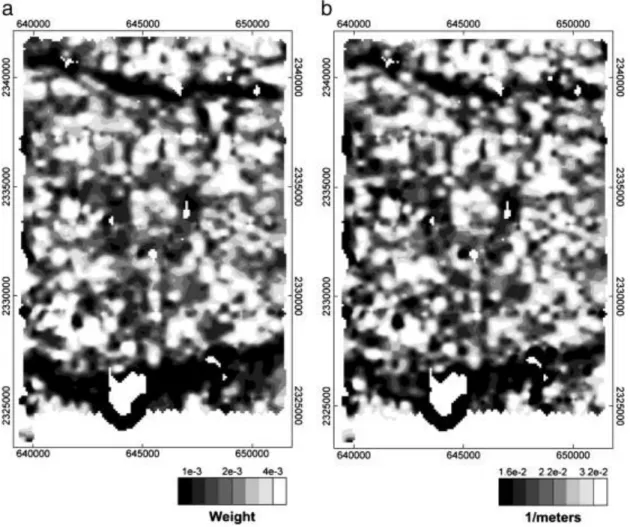
Each component can also be associated to a map of weight over the study area. This was obtained, for each component, plotting the absolute value of its weight at each measurement location. For instance, the weight map of the first component is shown in Fig. 4a.
The correlation between the weight map of the first component (Fig. 4a) and the map of the inverse of the flight height (Fig. 4b) is significant. It indicates that, to the first order, the amplitude variations caused by the variations of altitude of the receiver are explained by the first component of the SVD. Indeed, the first component represents the average decay; i.e. the more the ground clearance increases, the lower is the weight on the first component weight map. That is why the two East–West valleys at the north and the south of the area, where the helicopter could not fly as low as 30 m above the ground (flight lines oriented N–S), are highlighted by black, low weight values.
Some of the other weight maps are presented in Appendix B. In general, weight maps provide a cartographic overview showing where there are high weight values (bright zones) for a particular SVD component. Since the ―noisy components‖ were identified, further in the article, their weight maps will be used to characterize noise through the study area.
The appropriate separation between ―geological‖ and ―noisy‖ components presented above was not in fact so straightforward. We observed that the original components used to
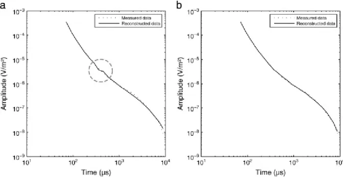
reconstruct decays appeared to introduce noise on certain decays. For instance, on Fig. 5a the reconstructed decay displays two small distortions at intermediate times. This occurred on several under-represented specific decays displaying an inflexion point (i.e. characteristic of the presence of a conductive sub-surface structure). The kind of reconstructed noise illustrated on Fig. 5a may therefore affect the reconstruction quality of under-represented or noisy
decays and should be addressed.
The solution adopted to improve the efficiency of the SVD was to reject the noisiest data before running the SVD. The method retained, after several tests, was to run a first SVD and reconstruct decays with the most obvious noise-free components only. We then compared the so-reconstructed decays to the measured ones in order to reject the decays which significantly differed from the reconstruction (i.e. the noisiest). On our dataset, 7 such noise-free
components of a total of 22 were retained. We assumed to explain with these 7 components, at least the amplitudes of 7 gates on each decay. Thus, if a decay had less than 7 coincident gates with the reconstruction (with a 10% tolerance), we decided to temporarily reject the decay. This procedure rejected from our dataset 1163 decays considered as ―too noisy‖. The
SVD ran on the remaining dataset then resulted in the 22 components shown in Fig. 2. Fig. 5 highlights the improvement obtained on the separation between geological signal and noise. Fig. 5b is the reconstruction of the same decay as in Fig. 5a, but, this time, using the
―geological components‖ of the reduced noise SVD (i.e. the components 1, 2, 3, 4, 5, 6, 8 previously identified). The reconstructed decay (Fig. 5b) does not contain noise anymore and better reproduces the measured one. This refinement of the SVD therefore improved the identification of the noise; this was also visually verified on other decays.
In the rest of the study, in order to keep acceptable parts of the 1163 temporarily rejected decays, we re-integrated them with the rest of the dataset (i.e. weights associated with each of the 22 components of each of the 1163 decays were calculated by inversion). The weights of all decays of the dataset were gathered in a single weight matrix.
3.4. Denoising procedure
The denoising process can be divided into three steps. In the following we develop: first, the rejection of spikes and oscillations, then the culling of decays affected by coupling noises, in two steps.
3.4.1. Gate rejection
In this part we focus on spikes and oscillations from mainly spherics, capacitive coupling and background noises.
We summed the previously identified ―geological components‖ in order to reconstruct decays. We compared numerically, gate by gate, each reconstructed decay to its corresponding
measured sounding (Fig. 6). For each time gate, if the difference between the measured and reconstructed amplitudes was greater than 10%, the gate was rejected from the measured decay. The 10% threshold has been considered, after several tests, taking into account that some geological information might still be contained in the rejected components and would thus have been skipped during the reconstruction. However, this threshold may also have the opposite effect and keep noisy gates, but, given the uncorrelated and random nature of noise, this opposite effect is theoretically pretty small. In order to correct this problem, we
additionally imposed on each decay at least three consecutive non-rejected gates, otherwise we rejected the gates. Moreover, three rejected gates on a measured decay were sufficient to reject the later delay times, i.e. we assumed to be below the noise level for the considered decay.
Fig. 6 shows the efficiency of the gate rejection process on two selected noisy decays. Whether the decay is affected by oscillations of different amplitudes (Fig. 6a, b) or by a shift in amplitude at intermediate times (Fig. 6b), the adopted SVD procedure successfully
identifies distortions within the decay curves. Identified aberrant amplitudes were rejected (black dots in Fig. 6). Since the ―noisy components‖ were statistically derived based on all soundings of the survey, the reconstruction and rejection process is effectively adapted to the entire dataset. This process allowed removing mainly the spherics and the oscillating part of capacitive coupling and background noises.
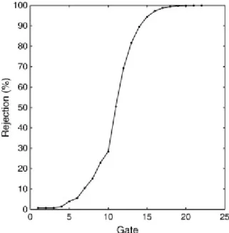
The quantitative effect of the gate rejection process is shown in Fig. 7. This shows that gate number 12 has been rejected in 70% of EM soundings. This statistical result thus provides an evaluation of the actual global noise level of the system in the geological environment of
Courtenay area. This also confirms that a large part of the data is affected by noise, as expected in an anthropized area. These results show clearly the efficiency of the SVD to recognize and reject undesired spikes and oscillations of different amplitudes from the data.
3.4.2. Decay rejection
Spherics and oscillations mainly from capacitive couplings and background noises were rejected by the gate rejection process. However, coupling noises may also distort the time constant and/or result in an amplitude shift of the decays measured above man-made installations. Those distorted decays create artifacts in the resistivity model and have to be culled. Nevertheless, their detection in airborne TDEM data remains difficult. Indeed, amplitude shifts affecting decays in their entirety cannot be differentiated from the effect of ground clearance variations and time constant distortions can hardly be differentiated from a normal TDEM pattern of a decay measured above a geological conductive structure. In this part we therefore focus on the characterization of those coupling noises.
3.4.2.1. Capacitive coupling noises detection
In this part, we focus on the characterization of capacitive coupling noises in order to cull the biased decays.
Capacitive coupling noise results in oscillations at early and intermediate times and may induce an amplitude shift on measured decays ( [Danielsen et al., 2003] and [Sørensen et al., 2000] ). Decays affected by capacitive coupling noises are therefore associated to high weight values on ―noisy components‖.
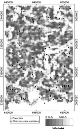
The sum of the weights of the ―noisy components‖ of each sounding is displayed in Fig. 8 and compared to the location of power lines and conductors seen on the flight videos, since the system had no power line monitor. It must be noted that this noise source inventory is certainly not exhaustive, given the difficulty to recognize a power line on the video. Moreover, it does not take into account possible buried pipelines (petroleum is currently extracted in the zone), but, to the first order, high weight values coincide well with the position of inventoried man-made installations, such as power lines going from one city to another. This processing therefore allows identifying the EM decays which are probably distorted by the presence of man-made installations and which should be considered as suspicious. We therefore used this information (Fig. 8) of perturbation of the signal by man-made installations to remove decays most likely biased by capacitive coupling noises. Thus, the manual cleaning phase is simplified thanks to this ―noise map‖ making it less time consuming and less subjective. However, it can be noticed that, for more clarity, we display only the sum of the weights of the ―noisy components‖, but the manual cleaning has to refer on each weight map of each ―noisy component‖, since a high value zone on one of these maps could be attenuated when summing.
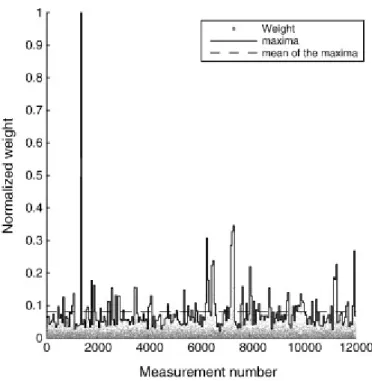
We can also propose a method to reject numerically the decays most likely biased by capacitive coupling noises. In order to target affected soundings, we ran a sliding maximum filter on weights of each identified ―noisy components‖. This filter was applied along the flight-lines. The size of the sliding window is a user-defined parameter and depends on the survey context; its influence is addressed in the following. For each successive position of the window, the filter substitutes weights within the window by their maximum value. For instance, the result of this filter applied on our dataset
with a sliding window of 50 soundings is shown in Fig. 9. The average of these maxima was then computed (horizontal dashed line in Fig. 9).
All decays with weights greater than the average were considered as being probably biased by
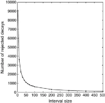
capacitive coupling noises and were therefore rejected. The number of rejected decays decreases as the sliding window size increases (Fig. 10). As some decays affected by coupling noises may be distorted without specific marked oscillations (i.e. associated with a lower values on weight maps of the ―noisy components‖), they could pass through this filter. Soundings located between two rejected ones within a distance of 150 m and which have not been ―seen‖ by the ―noisy components‖ were also removed. Location of the rejected decays for three sizes of the sliding window is displayed in Fig. 11 and compared to the map of the sum of the weights of the ―noisy components‖. Rejected soundings are well gathered, coherent from one map to another and also coherent with the ―noise map‖. This suggests that the method is well adapted to cull decays most probably biased by capacitive coupling noises. In this study, a sliding window of 50 soundings appears to be a good trade-off to cull those decays located above the man-made installations.
3.4.2.2. Galvanic coupling noises detection
Previous decay rejection phase, whether manual or numeric, is based on the analysis of the ―noisy components‖, which target only spikes and oscillations. Therefore, galvanic coupling noises resulting mainly in time constant distortions have theoretically not been well identified so far; decays affected by those noises present similar patterns to soundings measured above a geological conductive structure ( [Danielsen et al., 2003] and [Sørensen et al., 2000] ) and are rather explained by ―geological components‖ of the SVD. In this last part we focus on the characterization of galvanic coupling noises.
In order to locate the conductor responses, whether cultural or geological, we used some specifics SVD ―geological components‖. Identification of components which explain time constant distortions due to galvanic coupling noises was made through reconstruction tests on decays such as the one displayed in Fig. 5. In order to separate ―conductor-type‖ decays, we applied a K-means algorithm (McQueen, 1967) on weights of the selected ―geological components‖. This algorithm clusters data around k centroids (in our study k = 2). Fig. 12 displays the locations of ―conductor-type‖ decays (black dots) superimposed on the map of the sum of the weights of the ―noisy components‖. Most identified conductors are located in high weight value zones and have already been highlighted by the previous decay rejection process. Indeed, three phenomena can explain this:
–oscillations may distort the general pattern of the decay, then inducing high weight values on some ―geological components‖,
– overlays of several noises are possible, especially in an anthropized area,
–distortions of the time constant due to capacitive coupling noises may be explained by the selected ―geological components‖ too.
However, in order to detect decays affected by galvanic coupling noises, the positions of the other conductors had to be superimposed to the GIS map. Based on this ―conductor map‖, we were able to reject manually and quickly decays associated to locations coinciding with roads or other man-made installations. For instance, some particular soundings such as the one
circled (south of the area) had a very low noise level but coincided with the location of a man-made installation (Fig. 8). Of course, at this stage, the choice man-made by the user to reject or not such kind of ―conductor decay‖ is an important part of the work and cannot be automated.
4. Discussion–conclusion
The proposed SVD-based denoising process is a user-assisted method allowing filtering large amounts of TDEM data, based on a statistical approach. The procedure is efficient to reject noise from the data. One of its benefits is also to provide indicators for locating, mapping and characterizing noise through map overviews of the dataset. At least, this simplifies the manual cleaning phase. This cleaning can also be achieved with a numerical approach, as
demonstrated using a sliding maximum filter. The numerical approach can, for instance, be used in the field when surveying, in order to achieve rapid good quality filtering of the data and improved preliminary field inversions. However, the user decision undoubtedly remains the last and inescapable passage to decide whether a decay should be rejected or not.
The SVD procedure allows rejecting noises which cannot be reduced by filters applied on pre-stacked data. The case study on the Courtenay's area illustrated the efficiency and usefulness of the method to denoise data measured in an anthropized area. We were able to reject spikes and oscillations on decay curves, whatever their amplitudes. This result improves what is achieved with threshold methods on stacked data (HGG, 2011) and is complementary to threshold methods applied on pre-stacked data ( [Macnae et al., 1984] and [McCracken et al., 1984] ); the threshold being defined either according to experience or after several tests and a visual validation on some soundings. The threshold is therefore generally not well adapted to the entire dataset. This is not the case for the SVD filtering since the ―noisy components‖ were statistically derived based on all soundings of the survey. The SVD allowed also
locating the decays most likely affected by couplings with man-made installations, which are normally hardly recognized ( [Danielsen et al., 2003] and [Sørensen et al., 2000] ).
Identification of galvanic coupling noises was also improved through the mapping of decays associated with the presence of a conductor. Therefore, map indicators developed in our work provide efficient denoising tools or, at least make the manual editing less time consuming and less subjective.
The implementation of SVD method to denoise TDEM decays is however delicate and some choices were made in order to ensure the quality of results.
First, it has not been chosen to replace the measured decays by the reconstructed ones as it is done in gamma spectrometry (Hovgaard and Grasty, 1997). Indeed the smoothed decays obtained summing the ―geological components‖ can be slightly distorted, in terms of time constant, at noise level, as it can be seen in Fig. 6. We can't consider that the reconstructed amplitudes at noisy gates are those which would have been measured without noise.
Moreover, TDEM inversion is highly sensitive to slight decay slope variations. So, we rather decided to use the reconstructed decays for detecting and rejecting gates affected by noise.
Second, we decided to run the SVD on the entire decays (22 gates) though we know that there is mainly background noise on late time gates (Munkholm and Auken, 1996). Thus, early and intermediate time gates only could have been used to discriminate and characterize noise. We could have therefore run the SVD only on gates above a defined noise level. However, the SVD method requires that all decays have the same number of gates and reducing this number arbitrarily would have resulted in a loss of information on non-noisy decays. Moreover,
reducing the number of gates, we would have had fewer SVD components and not necessarily much less variations on decays; possibly, it would have been more difficult to discriminate between noise and geological components. Indeed, the variation of patterns from one decay to another is concentrated at early and intermediate gates rather than below the noise level.
Third, we took the absolute value of the gates since the uncorrelated negative values are inevitably due to noise and the induced variance would have needed several extra components to be explained. So, we would have had fewer components for explaining the useful patterns of decays. Moreover, negative values occur mostly at late delay times and are therefore of less interest than noise at intermediate times in a denoising procedure, as mentioned before.
Finally, our study was made in a rather simple geological context. With a more heterogeneous geology it could be useful to divide data into sub-datasets, corresponding to different
geological units. This could ―focus‖ the variance within each dataset and therefore tighten the statistical discrimination between noise and geological components. In this case, of course, enough data should be kept in each subset to achieve robust statistics. This is what is already proposed for gamma spectrometry data (Minty and McFadden, 1998).
One interrogation can be formulated to go further in the discussion: the filtering was made on raw stacked data. However, the application of the SVD on pre-stacked data could tentatively improve the signal-to-noise ratio in order to obtain better quality stacked data. A test was made but giving the inability to differentiate a spike due to spherics from oscillations of the background noise on the components since this differentiation occurs when summing the ―noisy components‖ and multiplying by the U matrix, this has not been thorough. A conjoint analysis of both components and weights could however solve this problem, which was however out of the scope of present study.
Acknowledgments
This work was carried out as part of a PhD co-financed by the Région Centre and the BRGM. Geophysical data on which the study is based were funded by the BRGM. Some figures of the article were produced using the software Geosoft©. We thank J. Macnae and an anonymous reviewer for constructive comments which helped improving the article.
References
Auken et al., 2007 E. Auken, J.A. Westergaard, A.V. Christiansen and K.I. Sørensen, Processing and inversion of SkyTEM data for high resolution hydrogeophysical surveys, Nineteenth International Geophysical Conference and Exhibition, ASEG, Perth, Western Australia (2007), 4p.
Auken et al., 2009 E. Auken, S. Violette, N. d'Ozouville, B. Deffontaines, K.I. Sørensen, A. Viezzoli and G. de Marsily, An integrated study of the hydrogeology of volcanic islands using helicopter borne transient electromagnetic: application in the Galápagos Archipelago. C.R.
Geoscience, 341 (2009), pp. 899–907
Bouchedda et al., 2010 A. Bouchedda, M. Chouteau, P. Keating and R. Smith, Sferics noise reduction in time-domain electromagnetic systems: application to MegaTEMII signal enhancement. Exploration Geophysics, 41 (2010), pp. 225–239.
Buselli and Cameron, 1996 G. Buselli and M. Cameron, Robust statistical methods for reducing spherics noise contaminating transient electromagnetic measurement.
Geophysics, 61 (1996), pp. 1633–1644.
Buselli et al., 1998 G. Buselli, J.P. Pik and H.S. Hwang, AEM noise reduction with remote referencing. Exploration Geophysics, 29 (1998), pp. 71–76.
Cull, 1991 J.P. Cull, Signal processing concepts for airborne SIROTEM data. Exploration
Geophysics, 22 (1991), pp. 97–100.
Danielsen et al., 2003 J.E. Danielsen, E. Auken, F. Jørgensen, V. Søndergaard and K.I. Sørensen, The application of the transient electromagnetic method in hydrogeophysical surveys. Journal of Applied Geophysics, 53 (2003), pp. 181–198.
Effersø et al., 1999 F. Effersø, E. Auken and K.I. Sørensen, Inversion of band-limited TEM responses. Geophysical Prospecting, 47 (1999), pp. 551–564.
Flis et al., 1989 M.F. Flis, G.A. Newman and G.W. Hohmann, Induced-polarization effects in time-domain electromagnetic measurements. Geophysics, 54 (1989), pp. 514–523.
Green, 1998 A. Green, The use of multivariate statistical techniques for the analysis and display of AEM data. Exploration Geophysics, 29 (1998), pp. 77–82.
HGG, 2011 HGG, Guide for processing and inversion of SkyTEM data in the Aarhus Workbench http://www.hgg.geo.au.dk/rapporter/guide_skytem_proc_inv.pdf (2011).
Hovgaard, 1997 J. Hovgaard, A new technique for airborne gamma-ray spectrometer data (Noise Adjusted Singular Value Decomposition) American Nuclear Sixth Topical Meeting on
Emergency Preparedness and Response, San Francisco, California (1997), pp. 123–127.
Hovgaard and Grasty, 1997 J. Hovgaard and R.L. Grasty, Reducing statistical noise in airborne gamma-ray data through spectral component analysis Fourth Decennial
International Conference on Mineral Exploration, Toronto, Canada (1997), pp. 753–764.
Jørgensen et al., 2003 F. Jørgensen, P.B.E. Sandersen and E. Auken, Imaging buried Quaternary valleys using the transient electromagnetic method. Journal of Applied
Geophysics, 53 (2003), pp. 199–213.
Junge, 1996 A. Junge, Characterization of and correction for cultural noise. Surveys in
Geophysics, 17 (1996), pp. 361–391.
Macnae et al., 1984 J.C. Macnae, Y. Lamontagne and G.F. West, Noise processing techniques for time-domain EM systems. Geophysics, 49 (1984), pp. 934–948.
McCracken et al., 1984 K.G. McCracken, J.P. Pik and R.W. Harris, Noise in EM exploration systems. Exploration Geophysics, 15 (1984), pp. 169–174.
McCracken et al., 1986 K.G. McCracken, M.L. Oristaglio and G.W. Hohmann, Minimization of noise in electromagnetic exploration systems. Geophysics, 51 (1986), pp. 819–832.
McQueen, 1967 J. McQueen, Some methods for classification and analysis of multivariate observations Fifth Berkeley Symposium on Mathematical Statistics and Probability, Berkeley,
California (1967), pp. 281–297.
Minty and McFadden, 1998 B. Minty and P. McFadden, Improved NASVD smoothing of airborne gamma-ray spectra. Exploration Geophysics, 29 (1998), pp. 516–523.
Munkholm and Auken, 1996 M.S. Munkholm and E. Auken, Electromagnetic noise
contamination on transient electromagnetic soundings in culturally disturbed environments.
Journal of Environmental and Engineering Geophysics, 1 (1996), pp. 119–127.
Nekut and Eaton, 1990 A.G. Nekut and P.A. Eaton, Effects of pipelines on EM soundings
60th SEG meeting, Expanded Abstracts, San Francisco, California (1990), pp. 491–494.
Palacky and West, 1991 G.J. Palacky and G.F. West, Airborne electromagnetic methods, M.N. Nabighian, Editor, Electromagnetic methods in applied geophysics, 02. Society of
Exploration Geophysicists (1991), pp. 811–879.
Press et al., 1992 W.H. Press, B.P. Flannery, S.A. Teukolsky and W.T. Vetterling, Numerical Recipes in C: The Art of Scientific Computing, (Second ed.), Cambridge University Press, Cambridge (1992).
Sørensen et al., 2000 K.I. Sørensen, E. Auken and P. Thomsen, TDEM in groundwater mapping — a continuous approach Symposium on the Applications of Geophysics to
Engineering and Environmental Problems, Arlington, Virginia (2000), pp. 485–491.
Sørensen and Auken, 2004 K.I. Sørensen and E. Auken, SkyTEM, A new high-resolution helicopter transient electromagnetic system. Exploration Geophysics, 35 (2004), pp. 191– 199.
Spies, 1988 B.R. Spies, Local noise prediction filtering for central induction transient electromagnetic sounding. Geophysics, 53 (1988), pp. 1068–1079.
Spies and Frischknecht, 1991 B.R. Spies and F.C. Frischknecht, Electromagnetic sounding, M.N. Nabighian, Editor, Electromagnetic methods in applied geophysics, 02. Society of
Exploration Geophysicists (1991), pp. 285–425.
Stephan and Strack, 1991 A. Stephan and K.M. Strack, A simple approach to improve S/N ratio for TEM data using multiple receivers. Geophysics, 56 (1991), pp. 863–869.
Strack et al., 1989 K.M. Strack, T.H. Harstein and H.N. Eilenz, LOTEM data processing for areas with high cultural noise levels. Physical of the Earth and Planet Interiors, 53 (1989), pp. 261–269.
Szarka, 1988 L. Szarka, Geophysical aspects of man-made electromagnetic noise in the earth — a review. Surveys in Geophysics, 9 (1988), pp. 287–318.
Viezzoli et al., 2010 A. Viezzoli, L. Tosi, P. Teatini and S. Silvestri, Surface water–
groundwater exchange in transitional coastal environments by airborne electromagnetics: the Venice Lagoon example. Geophysical Research Letters, 37 (2010), p. L01402.
Ward and Hohmann, 1988 S.H. Ward and G.W. Hohmann, Electromagnetic theory for geophysical applications, M.N. Nabighian, Editor, Electromagnetic methods in applied
Fig. 1. : Locations of the major cities in the study area (black outlined boxes) and the two valleys (written on white background).The rectangle shows the surveyed area.
Fig. 2. : Plots of the 22 SVD components. The first component represents the average decay and the subsequent components are successively the average of the residual. See text for detailed comments.
Fig. 3. : Plots of component 1 (dotted line), compared to plots in black line of (a) components 1 + 2, (b) components 1 + 7, (c) components 1 + 8 and (d) components 1 + 14 (multiplied by their eigenvalues).
Fig. 4. : Weight map of the first component (a) compared to the map of the inverse of the flight height (b).
Fig. 5. : Reconstruction of a decay measured above a conductor, (a) before with a dashed circle highlighting oscillations and (b) after rejecting the 1163 ―noisiest‖ decays (see text for details). Dotted and black curves represent respectively the measured decay and the
Fig. 6. : Effect of the gate rejection phase exemplified on two noisy decays: a decay affected mainly by oscillations (a) and a decay shifted at intermediate times (b). The black and gray curves represent respectively the measured and the reconstructed decay and black dots indicate the rejected gates.
Fig. 7. : Plots of the percentage of rejected measures as a function of the gate number. Black dots represent the data. The percentage of rejection increases with gate number since the signal-to-noise ratio decreases with time.
Fig. 8. : Location of the inventoried man-made installations seen on the flight video
superimposed on the map of the sum of the weights of the ―noisy components‖. Crosses and black dots correspond respectively to power lines and other man-made installations.
Fig. 9. : Example of sliding maximum filter applied on the normalized weights of the 18th component, for a window size of 50 soundings. Gray dots correspond to the normalized weights and black and dashed black lines represent respectively the envelope of the maxima and their average.
Fig. 10. : Number of rejected decays as a function of the window size of the sliding maximum filter. Black dots represent the data. The curve decreases with the interval size to obtain a unique maximum for an interval containing all the dataset.
Fig. 11. : Location of the rejected decays superimposed on the map of the sum of the weights of the ―noisy components‖ for a sliding maximum filter with a window size of 30, 50 and 70.
Fig. 12. : Conductor positions, obtained by application of the K-means algorithm, superimposed on the map of the sum of the weights of the ―noisy components‖.