HAL Id: hal-00296339
https://hal.archives-ouvertes.fr/hal-00296339
Submitted on 26 Sep 2007
HAL is a multi-disciplinary open access
archive for the deposit and dissemination of
sci-entific research documents, whether they are
pub-lished or not. The documents may come from
teaching and research institutions in France or
abroad, or from public or private research centers.
L’archive ouverte pluridisciplinaire HAL, est
destinée au dépôt et à la diffusion de documents
scientifiques de niveau recherche, publiés ou non,
émanant des établissements d’enseignement et de
recherche français ou étrangers, des laboratoires
publics ou privés.
Evidence of gravity waves into the atmosphere during
the March 2006 total solar eclipse
C. S. Zerefos, E. Gerasopoulos, I. Tsagouri, B. E. Psiloglou, A. Belehaki, T.
Herekakis, A. Bais, S. Kazadzis, C. Eleftheratos, N. Kalivitis, et al.
To cite this version:
C. S. Zerefos, E. Gerasopoulos, I. Tsagouri, B. E. Psiloglou, A. Belehaki, et al.. Evidence of gravity
waves into the atmosphere during the March 2006 total solar eclipse. Atmospheric Chemistry and
Physics, European Geosciences Union, 2007, 7 (18), pp.4943-4951. �hal-00296339�
www.atmos-chem-phys.net/7/4943/2007/ © Author(s) 2007. This work is licensed under a Creative Commons License.
Chemistry
and Physics
Evidence of gravity waves into the atmosphere during the March
2006 total solar eclipse
C. S. Zerefos1,3, E. Gerasopoulos1, I. Tsagouri1, B. E. Psiloglou1, A. Belehaki1, T. Herekakis1, A. Bais2, S. Kazadzis2,
C. Eleftheratos3, N. Kalivitis4, and N. Mihalopoulos4
1National Observatory of Athens, V. Pavlou & I. Metaxa, P. Penteli, 15236, Athens, Greece
2Aristotle University of Thessaloniki, Physics Department, Laboratory of Atmospheric Physics, Thessaloniki, Greece 3Foundation for Biomedical Research, Academy of Athens, Greece
4University of Crete, Chemistry Department, Environmental and Chemical Processes Laboratory, Crete, Greece
Received: 26 April 2006 – Published in Atmos. Chem. Phys. Discuss.: 31 May 2007
Revised: 12 September 2007 – Accepted: 18 September 2007 – Published: 26 September 2007
Abstract. This study aims at providing experimental
ev-idence, to support the hypothesis according to which the movement of the moon’s shadow sweeping the ozone layer at supersonic speed, during a solar eclipse, creates gravity waves in the atmosphere. An experiment was conducted to study eclipse induced thermal fluctuations in the ozone layer (via measurements of total ozone column, ozone pho-tolysis rates and UV irradiance), the ionosphere (Ionosonde Total Electron Content – ITEC, peak electron density height – hmF2), and the troposphere (temperature, relative humid-ity), before, during and after the total solar eclipse of 29 March 2006. We found the existence of eclipse induced dominant oscillations in the parameters related to the ozone layer and the ionosphere, with periods ranging between 30– 40 min. Cross-spectrum analyses resulted to statistically significant square coherences between the observed oscilla-tions, strengthening thermal stratospheric ozone forcing as the main mechanism for GWs. Additional support for a source below the ionosphere was provided by the amplitude of the oscillations in the ionospheric electron density, which increased upwards from 160 to 220 km height. Even though similar oscillations were shown in surface temperature and relative humidity data, no clear evidence for tropospheric in-fluence could be derived from this study, due to the modest amplitude of these waves and the manifold rationale inside the boundary layer.
Correspondence to: C. Zerefos
1 Introduction
Gravity waves (GWs) constitute an essential motion com-ponent of the atmospheric circulation due to their impor-tant contribution in the momentum and energy budget and in the wind systems of the atmosphere (Fritts and Alexan-der, 2003). Their role in weather, climate and atmospheric chemistry is very important. In particular, they can trans-port energy and momentum between different atmospheric regions and disturb the balanced state or initiate and modu-late convection and subsequent hydrological processes (e.g. Mapes, 1993). The initiated by GWs convection, can result to formation of clouds (e.g. orographic cirrus, polar strato-spheric and mesostrato-spheric; D¨ornbrack et al., 2002), modify chemistry, and trigger numerous processes (e.g. Voigt et al., 2000). During their dissipation phase, they contribute to the vertical transport and mixing of chemical species and influ-ence momentum and energy in the upper troposphere/lower stratosphere and in the mesosphere and lower thermosphere (e.g. Hays et al., 2003).
A varying number of sources are believed to generate GWs at lower levels of the atmosphere including topography, con-vective and frontal activity, wind shear and geostrophic ad-justment, while at greater heights their sources include non-linear wave-wave interactions, auroral currents, ion drag and Joule heating but also the differential heating of the atmo-sphere at dawn and dusk terminator and during solar eclipses (Fritts and Luo, 1993 and references therein).
Chimonas and Hines (1970) were the first to suggest that during a solar eclipse the disturbance of the heat balance along the supersonic travel of the trajectory of the moon’s shadow could generate GWs. The source of these waves was assumed to be either at higher altitudes e.g. at around 90 km
4944 C. Zerefos et al.: Gravity waves during the March 2006 total solar eclipse where molecular oxygen heating begins (Chimonas, 1970),
or at lower altitude e.g. water vapor IR absorption (Lamb waves) and the ground cooling (Chimonas and Hines, 1971; Chimonas, 1973). Morover, in both Chimonas (1970) and its subsequent follow on study of Firtts and Luo (1993), ther-mal cooling of the stratospheric ozone layer as the forcing function of GWs during a solar eclipse was considered. Eck-ermann et al. (2007), with their high-altitude global numeri-cal weather prediction model, recently simulated an induced radiative cooling rate in the stratosphere, 2–3 times larger than assumed in these earlier stratospheric bow wave models. In all cases, the source ambiguity makes subsequent experi-mental studies seeking evidence of eclipse-generated gravity waves, particularly complicated.
There have been a number of attempts to detect ground level atmospheric pressure waves resulting from solar eclipses. The periods of such waves range from the order of 1 min to 1 h or so, the decay times range from half the wave period upwards, and the ground level amplitude is unlikely to exceed 0.1 hPa, and is typically far less (Jones, 1999). In only few cases does the balance probability lie in favour of a detection of such waves (Jones, 1999; references therein). Anderson et al. (1972) reported on surface pressure fluctua-tions in the range 15–150 min and Seykora et al. (1985) found a surface pressure response with a period of about 4 h and a speed of 320 m s−1. The amplitudes of these waves were larger than those predicted by Chimonas (1970), but agree well with the 0.1–0.5 hPa range modelled recently by Ecker-mann et al. (2007).
A limited number of attempts to detect GW signals on total ozone have been made. Mims and Mims (1993) identified a sequence of 4–5 nearly uniformly spaced fluctuations, how-ever with small periods (4.5–7.2 min), on total ozone series, using a TOPS (Total Ozone Portable Spectrophotometer), but the linkage with eclipse induced GWs appears weak. Zerefos et al. (2000), deploying power spectral analysis on erythe-mal irradiance, revealed a significant oscillation in the ozone layer with a period of about 20 min.
In the ionosphere, waves with a period of 10–40 min have been measured at more than 500 km from the zone of total-ity (Singh et al., 1989), traveling at subsonic (Davis and da Rosa, 1970) or supersonic velocities (Hanuise et al., 1982). Lastly, a source location has been identified in the thermo-sphere at 170 km altitude due to reduced heating by absorp-tion of extreme ultraviolet solar radiaabsorp-tion, based on the anal-ysis of ionosonde measurements (Liu et al., 1998; Altadill et al., 2001; Sauli et al., 2006), while larger periods of about 1 h have also been reported (Altadill et al., 2001). Prior to those observations, the idea of an in-situ thermospheric wave source was highlighted by various modeling studies (Ridley et al., 1984; Roble et al., 1986; M¨uller-Wodarg et al., 1998). Despite decades of research, observational evidence for a characteristic bow-wave response of the atmosphere to eclipse passages remains equivocal (Eckermann et al., 2007). In this work, an attempt to shed light on the generation of
GWs during solar eclipses is made, with measurements at the three critical layers in the atmosphere namely the tropo-sphere, the stratosphere and the ionosphere. The main goal is to provide experimental evidence supporting the initial hy-pothesis that the cooling of the ozone layer in the stratosphere by the moon shadow travelling at supersonic speed during the eclipse, constitutes a source of gravity waves propagat-ing both upwards and downwards.
2 Instrumentation
Ultraviolet direct and global solar spectral measurements were performed at Kastelorizo (36◦09′N, 29◦35′E), Thessa-loniki (40◦38′N, 22◦57′E) and Athens (38◦03′N, 23◦52′E) using Brewer spectroradiometers (MKIII, MKII and MKIV, respectively). A map with the location of the above stations with regard to eclipse path and circumstances can be found in Gerasopoulos et al. (2007)1. The characteristics of the in-strument and details about their calibration procedures are described in detail by Bais et al. (1996). The three instru-ments followed the same measuring schedule on the eclipse day (29 March) and on the previous day. For this study the operating software of the instrument was modified to allow the alternating measurement (every 30 s) of global and direct spectral irradiance at 6 wavelengths between 302 and 320 nm that are used for measuring total column ozone and columnar SO2. These measurements were performed from 07:30 UTC
until 14:30 UTC. More details are given by Blumthaler et al. (2006) and Kazadzis et al. (2007).
Ozone photolysis frequencies (JO1D) have been also cal-culated from the Brewer spectroradiometer global irradi-ance measurements following the methodology described in Kazandzis et al. (2004). JO1D measurements have been also conducted at Finokalia, with a filter radiometer – Meteo-rologie Consult, Germany (Gerasopoulos et al., 2006). We have also used UV measurements from the Greek UV moni-toring network (http://www.uvnet.gr), equipped with NILU-UV multi-channel radiometers, providing NILU-UV irradiance at five wavelength bands centered at 305, 312, 320, 340 and 380 nm (Kazantzidis et al., 2007). Meteorological measure-ments at a number of sites including Kastelorizo and Fi-nokalia have been also conducted during the eclipse, as de-scribed by Founda et al. (2007).
Ionospheric observations from the National Observatory of Athens Digisonde (http://www.iono.noa.gr) were used for the investigation of the ionospheric response to the solar eclipse of 29 March 2006 over Athens (38◦00′N, 23◦30′E). In particular, calculations of electron density profiles up to 1000 km, obtained under a vertical incidence ionospheric sounding campaign, were used for the derivation of the peak electron density height, hmF2, and the estimation of the
1Gerasopoulos, E., Zerefos, C. S., Tsagouri, I., et al.: The To-tal Solar Eclipse of March 2006: Overview, Atmos. Chem. Phys. Discuss., in preparation, 2007.
Ionosonde Total Electron Density, ITEC., (Gerasopoulos et al., 20071). In addition, the electron densities at fixed iono-spheric altitudes zones were calculated, enabling the study of electron density variations as a function of time and altitude (Altadill et al., 2001).
3 Analysis and results
3.1 Methodology
Observations from various atmospheric layers were analyzed deploying Spectral Fourier Analysis, in an effort to investi-gate the possible detection of GWs propagating in different atmospheric heights during the 29 March 2006 Total Solar Eclipse. In this study we have used the following param-eters: i. total ozone over Kastelorizo, Athens and Thessa-loniki, mainly as an index of the disturbance in the strato-spheric ozone layer, additionally supported by ozone photol-ysis rates JO1D and UV (305 nm) irradiance measurements, ii. the Ionosonde Total Electron Content (ITEC) as an indi-cator for the total ionosheric ionization disturbances, and the peak density height of the F2 layer (hmF2) as a first indicator for the propagation of wave-like motions in the ionosphere, iii. ground measurements of temperature and relative humid-ity at Kastelorizo and Finokalia.
As input data for the spectral analysis, we have used the residual time series of the above parameters. Residuals have been calculated by applying polynomial fittings to the ini-tial time series, to remove the combined effect of the eclipse and the diurnal variability of each parameter. We have cho-sen the maximum period during the eclipse that almost cloud free conditions were encountered at all sites, so that the same period would be used for all parameters (10:00–11:52 UTC). Short-time contamination by light and temporary cloudiness or a very few cases of aircraft contrails (evidenced mainly on actinometric data) at each site, has been also removed by substituting the respective residual values with zeroes. For all parameters except for the ionospheric, 1 min time resolution data were available. Ionospheric parameters were available with a 4 min time resolution.
Because of the short duration of the investigated period, we have used the zero-padding method which consists in adding zeros at the end of the time series, to improve fre-quency resolution of the resulting power spectra, thus en-hancing our ability to estimate the signal’s period more ac-curately and discriminate close periodicities.
3.2 Investigation of observed oscillations in the ozone layer For the period between 10:00 and 13:00 UTC, the total ozone column at Kastelorizo was changing on the day before the eclipse from about 335 DU down to about 325 DU, and on the day of the eclipse it was increasing from about 290 DU to 305 DU (Kazadzis et al., 2007). An increase of total ozone
by the end of the eclipse in the range 5–24 DU is also re-confirmed from the NILU-UV measurements in a number of stations (Kazantzidis et al., 2007). During the course of the eclipse, a gradual decrease in total ozone at Kastelorizo, followed by an almost symmetric increase after the totality is observed (Fig. 1a, upper graph). This effect has been re-ported earlier by Zerefos et al. (2000), and it was attributed partly to the limb darkening effect and partly to the in-creasing influence of direct irradiance by the diffuse radi-ance entering the field of view of the total ozone instru-ments. Blumthaler et al. (2006), confirmed this finding by calculating a correction for total ozone due to limb darken-ing. This correction was found to be very small (less than 0.01%). Therefore the most possible reason for the reduced total ozone values during the eclipse is the contamination of direct irradiance measurements by the diffuse radiation (Kazadzis et al. 2007).
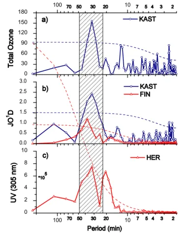
Total ozone residuals at Kastelorizo are shown in Fig. 1a (lower graph). A Savitzky-Golay smoothing (2nd order mov-ing polynomial, 10 points) is also used for the better visual-ization of the lower frequency fluctuations. The two vertical lines in Fig. 1a correspond to sun coverage by the moon of more than 70%, corresponding roughly to a reduction in di-rect irradiance measurements (under normal conditions) at airmass factors of more than 3, which are usually discarded in the standard Brewer total ozone measurements (Kazadzis et al., 2007). This effect results in a smooth continuous re-duction of the ozone values, which is removed by the applied polynomial fit, thus the eclipse induced oscillations in the total ozone data are added on top of this smooth reduction of total ozone. The peak-to-peak amplitude of the residuals is about 2–3.5% of the total ozone averaged over the same period, and three main oscillations were observed starting 30 min after the first contact. Cloud development a little be-fore last contact prevented the further capture of the evolution of the waves.
Since these oscillations are observed mainly during the measurement interval influenced by the diffuse radiation, we have used two additional parameters to express total ozone variability and confirm the existence of the oscillations, the photolysis rate of the reaction of O3to O(1D), JO1D and UV
irradiance at 305 nm. JO1D is mainly sensitive to the total column ozone, but also to the total aerosol optical depth, aerosol growth with relative humidity and by clouds depend-ing on the optical depth of the cloud (Ruggaber et al., 1994). Moreover, UV irradiance at 305 nm exhibits maximum ozone absorption compared to higher wavelengths provided by the NILU-UV radiometers (Kazantzidis et al., 2007). It should be noted that the effect of diffuse irradiance that was regarded as the reason for the biased total ozone measurements during the eclipse, has no influence on the Brewer irradiance mea-surements, and consequently on the derived JO1D data.
JO1D measurements at Kastelorizo and Finokalia are shown in Figs. 1b and c (upper graphs) with the respec-tive polynomial fittings. JO1D residuals are presented in the
4946 C. Zerefos et al.: Gravity waves during the March 2006 total solar eclipse 80 100 120 140 160 180 200 220 240 260 280 300 320 10:00 10:10 10:20 10:30 10:40 10:50 11:00 11:10 11:20 11:30 11:40 11:50 12:00 -15 -10 -5 0 5 10 15 20 25 30 -5 -4 -3 -2 -1 0 1 2 3 -20 -15 -10 -5 0 5 10 15 20 25 30 35 40 10:00 10:10 10:20 10:30 10:40 10:50 11:00 11:10 11:20 11:30 11:40 11:50 12:00 -3 -2 -1 0 1 2 -10 -5 0 5 10 15 20
Fig. 1. (a) Upper: total ozone over Kastelorizo during the eclipse
and second order polynomials fitted on the data, Lower: total ozone residuals and a Savitzky-Golay (2nd order moving polynomial, 10 points) smoothing line. The two vertical lines correspond to sun coverage by the moon of more than 70% and residuals and smooth-ing line dursmooth-ing this period are presented by dot and thin (red, contin-uous) lines, respectively, (b) Upper: JO1D at Kastelorizo (KAST) during the eclipse and a third order polynomial fitted on the data, Lower: JO1D residuals and a Savitzky-Golay smoothing line, and
(c) Upper: JO1D at Finokalia (FIN) during the eclipse and second
order polynomials fitted on the data, Lower: JO1D residuals and a Savitzky-Golay smoothing line. Time in UTC.
100 10 100 10 0 2 4 6 8 10 0.0 0.5 1.0 1.5 2.0 2.5 3.0 0 30 60 90 120 150 180
Fig. 2. Power Spectrum Analysis applied on the residuals of
vari-ous atmospheric parameters during the eclipse (10:00–11:52 UTC, 29 March 2006); Y-axes correspond to the spectral estimates for the following parameters: (a) total ozone at Kastelorizo (KAST), (b) JO1D at Kastelorizo (blue line + circles) and Finokalia (FIN, red line + triangles), (c) UV (302 nm) at Heraklion (HER, red line + triangles), Lefkosia (LEF, blue line + circles) and Ioannina (IOA, green line + triangles reversed). Similarly colored dash lines rep-resent the 95% confidence limits of each spectrum. Axes in (c) are divided by 105.
lower graph of Figs. 1b and c, and the smoothing line reveals oscillations with similar characteristics. Indeed, the main os-cillations found in total ozone at Kastelorizo are reproduced with a certain lag in JO1D at the same station, but also in dis-tance from totality, at Finokalia. The average peak-to-peak amplitude of the residuals is about 8% and 10% of the JO1D over the same period, at Kastelorizo and Finokalia, respec-tively, however corresponding to almost half amplitudes for the more distant from totality station (Finokalia), given the different levels of JO1D at the two sites.
The oscillations are further investigated with Spectral Fourier Analysis (Fig. 2). The power spectrum of total ozone over Kastelorizo reveals a significant oscillation (99% con-fidence level, not shown) with a period in the range 28– 38 min (Fig. 2a). A secondary oscillation is found at peri-ods 12–13 min which approaches the 95% confidence level.
0 12 24 36 48 60 72 84 96 108 120 0 200 400 600 800 1000 0 12 24 36 48 60 72 84 96 108 120 -100 -80 -60 -40 -20 0 20
Fig. 3. Hourly records of Dstindex (http://swdcwww.kugi.kyoto-u.
ac.jp/dstdir/index.html), as indicator of the geomagnetic activity level (top panel) and of AE index (http://swdcwww.kugi.kyoto-u. ac.jp/aedir/index.html) indicating the level of the auroral electrojets intensity (bottom panel) for the time interval 27–31 March 2006. The blue dash lines represent indicative thresholds for the identifi-cation of considerable geomagnetic/magnetospheric disturbances.
The same process was applied on the total ozone time series at Thessaloniki (not shown). A significant oscillation (95% confidence level) with a period of 28–32 min was found, de-noting the spatial extent of the ozone layer perturbation. The amplitude of the residuals was found to be in the order of 3– 4% of the total ozone, averaged over the same period. The influence of clouds was much more extended on total ozone over Athens, thus hindering the attribution of fluctuations to GWs. The discussed range of periodicities could not be iden-tified on the previous and next day spectra of the total ozone series over all sites (for the same time interval; not shown).
The power spectrum of JO1D at Kastelorizo reveals the same features with total ozone at the same station, allow-ing its use as a proxy for total ozone variability. The same spectrum is also revealed when 4-min averages are first ex-tracted (not shown). The latter ensures that no bias is im-posed on the cross-spectrum between the 4 min averages of total ozone and the ionospheric parameters (Sect. 3.3). The power spectrum of JO1D at Finokalia shows a peak at 32– 45 min (99% significance level, not shown), while the UV ir-radiance at 305 nm spectrum at Heraklion, reveals two peaks at 28–45 min and 17–23 min. Similar oscillations were found in UV irradiance at distant stations from the peak eclipse, namely Ioannina and Nicosia (Kazantzidis et al., 2007).
Overall, a main oscillation with period in the range 30– 40 min is found at a number of stations with independent measurements of total ozone column and its proxies JO1D and UV irradiance, denoting an extended thermal strato-spheric ozone disturbance.
3.3 Investigation of observed oscillations in the ionosphere This solar eclipse took place under low geomagnetic and magnetospheric activities, providing clear advantage for the
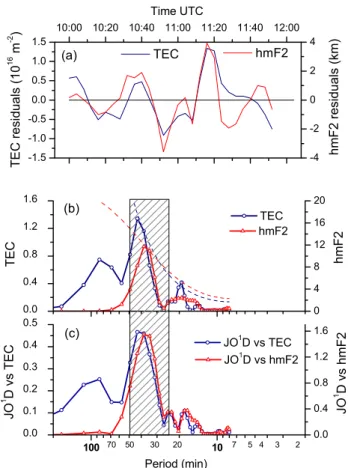
-1.5 -1.0 -0.5 0.0 0.5 1.0 1.5 10:00 10:20 10:40 11:00 11:20 11:40 12:00 -4 -2 0 2 4 h m F 2 re si d u a ls (km) T E C re si d u a ls (1 0 1 6 m -2 ) TEC Time UTC (a) hmF2 0.0 0.4 0.8 1.2 1.6 0 4 8 12 16 20 100 10 0.0 0.1 0.2 0.3 0.4 0.5 JO 1 D v s h mF 2 JO1D vs TEC Period (min) JO 1 D vs T EC (c) 0.0 0.4 0.8 1.2 1.6 TEC T EC (b) JO1D vs hmF2 70 50 30 20 7 5 4 3 2 hmF2 h m F 2
Fig. 4. (a) Ionosonde TEC and hmF2 residuals, (b) Spectrum
Anal-ysis applied on the residuals; Y-axes correspond to the spectral es-timates of the parameters and similarly colored dash lines represent the 95% confidence limits of each spectrum, (c) Cross Spectrum Analysis between JO1D at Kastelorizo and ionospheric parameters; Y-axes correspond to the amplitude of the cross-spectrum for the following pairs: JO1D vs Ionosonde TEC (blue line + circles) and JO1D vs hmF2 (red line + triangles).
identification of signals from solar eclipse induced GWs in the ionosphere (Fig. 3). In particular, the geomagnetic activ-ity remained low, since the Dst index values ranged above −30 nT during the whole week (27–31 March 2006), and the same holds for the magnetosheric activity. Some moder-ate excursions in AE index (Mayaud, 1980) recorded in very early morning or very late evening hours the days prior to the eclipse day, cannot impose an effect in the ionosphere over Athens at the local time of the eclipse occurrence (Pr¨olss, 1995).
The complete evolution of ionospheric parameters dur-ing the eclipse is thoroughly discussed by Gerasopoulos et al. (2007)1. Here we focus on the oscillations observed in ITEC and hmF2 presented in Fig. 4a. Three main oscil-lations are found almost in coincidence with those of total ozone, however the lower time resolution of these measure-ments and the complexity of the exact GWs source (in the horizontal and the vertical), does not allow the estimation of
4948 C. Zerefos et al.: Gravity waves during the March 2006 total solar eclipse 160 180 200 0.0 0.1 0.2 0.3 0.4 0.5 0.6 0.7 0.8 0.9 1.0 160 180 200 0.0 0.1 0.2 0.3 0.4 0.5 0.6 0.7 0.8 0.9 1.0
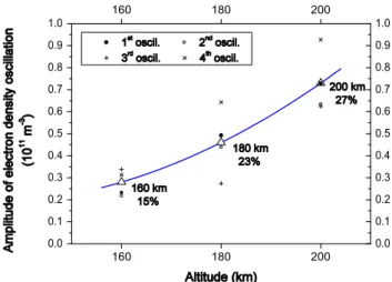
Fig. 5. Amplitudes of the electron density oscillations, calculated
as the difference between successive minima and maxima at fixed altitudes (160, 180 and 200 km). Triangles represent the average amplitude of four oscillations at each altitude accompanied by the respective regression line (blue line), while each individual oscil-lation is shown with different symbol (see label). The percentage below the respective altitudes expresses the standardized to the av-erage electron density (between first contact and maximum occul-tation) amplitude.
a reliable propagation velocity. The peak-to-peak amplitude of the ITEC residuals is 10–15% of the ITEC averaged over the eclipse period, while for hmF2 it is about 2%. The power spectra of ITEC and hmF2 are shown in Fig. 4b. Signifi-cant oscillations (95% confidence level) in the range 34–43 and 34–38 min are revealed for ITEC and hmF2, respectively. An additional peak is observed on the ITEC spectrum at 18– 20 min. Power spectra were also calculated for all “quiet” geomagnetic conditions on days between 27 and 31 March 2006, and no significant fluctuations were found, denoting that the 29 March periodicities were indeed related to solar eclipse effects.
Cross-Spectrum Analysis has been applied between JO1D at Kastelorizo and the ionospheric parameters. The ampli-tude of the cross spectra for the pairs JO1D vs ITEC and JO1D vs hmF2 is shown in Fig. 4c. A very distinct
co-variance between the frequency components corresponding to the ∼40 min periodicity is found in both spectra. Signifi-cantly high square coherences were calculated, 0.93 and 0.96 for JO1D vs ITEC and JO1D vs hmF2, respectively, demon-strating that the ionospheric oscillations are probably driven by GWs initially formed in the stratosphere.
Variation of electron density amplitudes with height: Elec-tron density variations at fixed ionospheric altitude zones of 20 km depth were additionally used to further speculate on the main source of GWs that have reached ionospheric heights. Consistent fluctuations with maximum amplitude in the altitude range of 200–220 km were observed during the first phase of the eclipse (Gerasopoulos et al., 20071). Such
oscillations were previously reported in the literate and are attributed to solar eclipse induced GWs during or after the solar eclipse (Altadill et al., 2001; Sauli et al., 2006). In this case, the fluctuations were considerably attenuated dur-ing the solar reappearance phase. The spectrum analysis (not shown) depicted a dominant periodicity of 15–18 min, coin-ciding with the higher frequency oscillations in total ozone and ITEC.
The change in the amplitude of these oscillations was used to speculate on the location of the GWs source responsible for the ionospheric signal. The amplitude of these oscil-lations was calculated as the difference between successive minima and maxima of the electron densities at the fixed tude zones. These oscillations were clearly present in the alti-tude range 140–220 km. However, the 140–160 km zone was not included in our discussion here in order to keep the E-layer conditions clearly out of the analysis, since the electron concentration is very low and the detection of oscillations is ambiguous. Moreover, no such analysis was performed above 220 km since the main response of the ionosphere to the eclipse was gradually diminished from that height up (Gerasopoulos et al., 20071).
The amplitude of each of the four oscillations that can be identified with relative good precision, as well as the aver-age amplitude per altitude is presented in Fig. 5. A tendency of increasing amplitude with altitude is clearly evidenced in both raw and standardized amplitudes, a result consistent with the effect of density decrease with height on the ampli-tude of a vertically propagating wave (Fritts and Luo, 1993). In summary, taking into account that the observed oscil-lations i) are clearly present in the ionospheric height range 140–220 km, ii) are well attenuated above 220 km, iii) they have the same period at each height, iv) they have an impor-tant vertical propagation component, with increasing ampli-tude with height and v) are not of auroral origin, one could ar-gue that they seem to originate from below the studied iono-spheric heights. The above characteristics lie in favour of propagating waves attributed to the movement of the cooled spot produced by the moon’s shadow in the ozone layer. 3.4 Investigation of observed oscillations in the
tropo-sphere
The identification of GWs in the troposphere is a much more difficult task. Especially inside the boundary layer (BL), any fluctuations are subject to multiple rationales and increased uncertainty, related to meteorological or other local scale fac-tors that may well mask the signal imposed by the propaga-tion of GWs down to the surface.
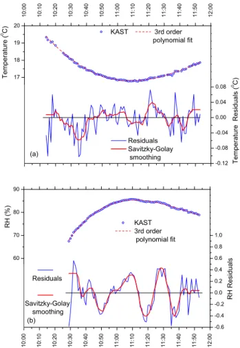
We have used the temperature record at Kastelorizo to de-tect any fluctuations from GWs near the surface. The temper-ature drop of 2.3◦C at Kastelorizo is shown in Fig. 6a (upper graph) accompanied by a polynomial fitting. Temperature residuals were calculated and are presented in Fig. 6a. (lower graph). The three oscillations seen in total ozone are also
12 13 14 15 16 17 18 19 20 1 0 :0 0 1 0 :1 0 1 0 :2 0 1 0 :3 0 1 0 :4 0 1 0 :5 0 1 1 :0 0 1 1 :1 0 1 1 :2 0 1 1 :3 0 1 1 :4 0 1 1 :5 0 1 2 :0 0 -0.12 -0.08 -0.04 0.00 0.04 0.08 0.12 0.16 0.20 0.24 T e mp e ra tu re R e si d u a ls ( 0 C ) T e mp e ra tu re ( 0C ) KAST 3rd order polynomial fit (a) Residuals Savitzky-Golay smoothing 1 0 :0 0 1 0 :1 0 1 0 :2 0 1 0 :3 0 1 0 :4 0 1 0 :5 0 1 1 :0 0 1 1 :1 0 1 1 :2 0 1 1 :3 0 1 1 :4 0 1 1 :5 0 1 2 :0 0 30 40 50 60 70 80 90 -0.6 -0.4 -0.2 0.0 0.2 0.4 0.6 0.8 1.0 1.2 1.4 1.6 1.8 R H R e s id u a ls R H (% ) KAST 3rd order polynomial fit (b) Residuals Savitzky-Golay smoothing
Fig. 6. (a) Upper panel: Temperature at Kastelorizo during the
eclipse (open circles) and a third order polynomial fitted on the data (dash red line), (b) Upper panel: The same for RH at Kastelorizo. Lower panels in (a) and (b): Residuals of each parameter (blue line-dots) and a Savitzky-Golay (2nd order moving polynomial, 10 points) smoothing line (continuous red line). Time in UTC.
served in surface temperature with a 5–10 min lag, however the peak-to-peak amplitude of the residuals is rather small ∼0.1◦C or 0.6% of the temperature averaged over the eclipse period, which is same order of magnitude with the sensors accuracy (±0.1◦C; Founda et al., 2007). This amplitude is
one order of magnitude lower than that predicted by Ecker-mann et al. (2007).
To exclude relation of this signal to instrumental noise and overcome a possible lack of confidence in the temperature oscillations we have repeated the same analysis with rela-tive humidity, RH (Fig. 6b). The residuals shown in Fig. 6b (lower graph) once more reveal the three dominant oscilla-tions and the peak-to-peak amplitude is ∼1% (absolute) or 1.2% of the RH averaged over the eclipse period. The accu-racy of the RH sensor is ±1%, so once more the amplitude of RH signal is comparable to the instrumental accuracy, how-ever, the fact that the oscillations are very distinct and are observed in both temperature and RH enhances our
confi-100 10 0.000 0.001 0.002 0.003 0.004 0.005 0.006 0.007 0.008 100 10 0.0 0.2 0.4 0.6 0.8 1.0 1.2 1.4
Fig. 7. Spectrum Analysis on temperature residuals and Cross
Spec-trum Analysis between JO1D and temperature at Kastelorizo. Y-axes correspond to the spectral and cross spectral estimates, and the colored dash line represents the 95% confidence limits of the spec-trum.
dence. It should be also noted here that averaging over 1 min intervals (measurements recorded every 20 s) has as a result to reduce the uncertainty both in temperature and RH mea-surements, and this is easily observed in Fig. 6a and b, where the noise is well separated from the oscillations.
The power spectrum of temperature at Kastelorizo is shown in Fig. 7 and a significant periodicity (95% confi-dence level) in the range 28–38 min is revealed. Similar os-cillations, with modest wave amplitudes ∼0.1◦C, were found in the spectra of the temperature time series at other sites namely Finokalia-Crete and Penteli-Athens (not shown). The cross spectrum between JO1D and temperature (Fig. 7) shows a strong covariance around the 30 min periodicity with significantly high square coherence, 0.97.
Concluding, even though distinct oscillations are observed in surface temperature data at various sites, additionally re-confirmed by similar relative humidity periodicity, there is no clear evidence for GWs in the troposphere. Especially inside the boundary layer, manifold rationale could be provided for such transient perturbations in temperature and more param-eters should be monitored and examined to draw safe con-clusions.
4 Summary – conclusions
Definite observational evidence for a characteristic bow-wave response of the atmosphere to solar eclipse passages, despite model calculations at various altitudes, has been still ambiguous. In this paper, we have provided combined ex-perimental evidence to support the initital hypothesis of Chi-monas and Hines (1970) that the cooling of ozone layer in the stratosphere by the supersonic travel of the moon’s shadow during an eclipse, constitutes a source of gravity waves propagating both upwards and downwards. To ex-amine the above, concurrent measurements at three critical
4950 C. Zerefos et al.: Gravity waves during the March 2006 total solar eclipse layers in the atmosphere namely in the troposphere, in the
stratosphere and in the ionosphere, were conducted.
Spectral Fourier Analysis revealed a dominant oscillation with period in the range 30–40 min in total ozone column over Kastelorizo (100% maximum occultation), but also at larger distances, with less sun coverage (Thessaloniki, 75% maximum occultation). It is expected that ozone in the upper stratosphere, where it maximizes and is in radiative equilib-rium, would respond more rapidly to the transient cooling due to the eclipse of the sun. The eclipse induced ozone layer thermal disturbance was endorsed by JO1D and UV ir-radiance (305 nm) measurements, both sensitive to columnar ozone variability, yet denoting a spatially extended propaga-tion of the GWs with regard to the totality axis.
The 30–40 min oscillation was also evident in the spectra of the Ionosonde Total Electron Content (ITEC) and the peak electron density height in the ionosphere (hmF2). Cross-spectrum analysis between total ozone and the ionospheric parameters depicted high covariance in this range of periods. The initial argument that the source of the perturbation orig-inates below the ionosphere was ratified by the fact that the amplitude of the electron density oscillation increased up-wards from 160 to 220 km, which is expected for a vertically propagating wave inside a mean of decreasing with height density.
The identification of the GWs oscillation in the tropo-sphere has been attempted with records of surface temper-ature and relative humidity. Distinct oscillations were ob-served in both parameters within the period range of our in-terest, at various sites. However, the amplitude of these oscil-lations has been modest and in the same order of magnitude with the sensor’s accuracy. It should be kept in mind that the intensity of the waves downwards could be considerably suppressed by the fact that the propagation takes place in a denser mean, and that inside the BL any periodical signal in the parameters subjects to manifold rationale also controlled by meteorological or other local scale factors. The above do not allow us to draw safe conclusions on the influence of eclipse induced GWs in the troposphere, and should be taken under consideration for future experiments planning. Acknowledgements. The authors would like to thank the two
anonymous reviewers for their insightful comments and S. Eckermann for his valuable suggestions. The Dst and AE indices’ records used in this analysis were obtained from the World Data Center for Geomagnetism, Kyoto archives (http://swdcwww.kugi.kyoto-u.ac.jp/).
Edited by: P. Monks
References
Altadill, D., Sole, J. G., and Apostolov, E. M.: Vertical structure of a gravity wave like oscillation in the ionosphere generated by the solar eclipse of August 11, 1999, J. Geophys. Res., 106(A10), 21 419–21 428, 2001.
Anderson, R. C., Keefer, D. R., and Myers, O. E.: Atmospheric pressure and temperature changes during the 7 March 1970 solar eclipse, J. Atmos. Sci., 29, 583–587, 1972.
Bais, A. F., Zerefos, C. S., and McElroy, C. T.: Solar UVB measure-ments with the double and single monochromator Brewer ozone spectroradiometers, Geophys. Res. Lett., 23, 833–836, 1996. Blumthaler, M., Bais, A., Webb, A., Kazadzis, S., Kift, R.,
Kouremeti, N., Schallhart, B., Kazantzidis, A.: Variations of so-lar radiation at the Earth’s surface during the total soso-lar eclipse of 29 March 2006, in: Remote Sensing of Clouds and the At-mosphere XI, edited by: Slusser, J. R., Sch¨afer, K., Comer´on, A., Proceedings of the SPIE, Vol. 6362, doi:10.1117/12.689630, 2006.
Chimonas, G.: Internal gravity-waves motions induced in the Earth’s atmosphere by a solar eclipse, J. Geophys. Res., 75, 5545–5551, 1970.
Chimonas, G.: Lamb waves generated by the 1970 solar eclipse, Planetary Space Science, 21, 1843–1854, 1973.
Chimonas, G. and Hines, C. O.: Atmospheric gravity waves in-duced by a solar eclipse, J. Geophys. Res., 75, p. 875, 1970. Chimonas, G. and Hines, C. O.: Atmospheric gravity waves
in-duced by a solar eclipse, 2, J. Geophys. Res., 76(28), 7003–7005, 1971.
Davis, M. J. and da Rosa, A. V.: Possible detection of atmospheric gravity waves generated by the solar eclipse, Nature, 226, p. 1123, 1970.
D¨ornbrack, A., Birner, T., Fix, A., Flentje, H., Meister, A., Schmid, H., Browell, E. V., and Mahoney, M. J.: Evi-dence for inertia gravity waves forming polar stratospheric clouds over Scandinavia, J. Geophys. Res., 107(D20), 8287, doi:10.1029/2001JD000452, 2002.
Eckermann, S. D., Broutman, D., Stollberg, M. T., Ma, J., Mc-Cormack, J. P., and Hogan, T. F.: Atmospheric effects of the total solar eclipse of 4 December 2002 simulated with a high-altitude global Model, J. Geophys. Res., 112, D14105, doi:10.1029/2006JD007880, 2007.
Founda, D., Melas, D., Lykoudis, S., Lysaridis, I., Kouvarakis, G., and Petrakis, M.: The effect of the total solar eclipse of March 29, 2006 on meteorological variables in Greece, Atmos. Chem. Phys. Discuss., 7, 10 631–10 667, 2007.
Fritts, D. C. and Luo, Z.: Gravity wave forcing in the middle at-mosphere due to reduced ozone heating during a solar eclipse, J. Geophys. Res., 98(D2), 3011–3021, 1993.
Fritts, D. C. and Alexander, M. J.: Gravity wave dynamics and effects in the middle atmosphere, Rev. Geophys., 41(1), 1003, doi:10.1029/2001RG000106, 2003.
Gerasopoulos, E., Kouvarakis, G., Vrekoussis, M., Donoussis, C., Kanakidou, M., and Mihalopoulos, N.: Photochemical ozone production in the Eastern Mediterranean, Atmos. Environ., 40, 3057–3069, doi:10.1016/j.atmosenv.2005.12.061, 2006. Hanuise, C., Broche, P., and Ogubazghi, G.: HF Doppler
observa-tions of gravity waves during the 16 February 1980 solar eclipse, J. Atmos. Solar-Terr. Phys., 44, 963–966, 1982.
Hays, P. B., Kafkalidis, J. F., Skinner, W. R., and Roble, R. G.:
A global view of the molecular oxygen night glow, J. Geophys. Res.-Atmos., 108(D20), 4646, doi:10.1029/2003JD003400, 2003.
Jones, B. W.: A search for atmospheric pressure waves from the total solar eclipse of 9 March 1997, J. Atmos. Solar-Terr. Phys., 61, 1017–1024, 1999.
Kazadzis, S., Topaloglou, C., Bais, A. F., Blumthaler, M., Balis, D., Kazantzidis, A., and Schallhart, B.: Actinic flux and O1D pho-tolysis frequencies retrieved from spectral measurements of irra-diance at Thessaloniki, Greece, Atmos. Chem. Phys., 4, 2215– 2226, 2004,
http://www.atmos-chem-phys.net/4/2215/2004/.
Kazadzis, S., Bais, A., Kouremeti, N., Blumthaler, M., Webb, A., Kift, R., Schallhart, B., and Kazantzidis, A.: Effects of total solar eclipse of 29 March 2006 on surface radiation, Atmos. Chem. Phys. Discuss., 7, 9235–9258, 2007,
http://www.atmos-chem-phys-discuss.net/7/9235/2007/. Kazantzidis, A., Bais, A. F., Emde, C., Kazadzis, S. and Zerefos, C.
S.: Attenuation of global ultraviolet and visible irradiance over Greece during the total solar eclipse of 29 March 2006, Atmos. Chem. Phys. Discuss., 7, 13475–13501, 2007,
http://www.atmos-chem-phys-discuss.net/7/13475/2007/. Liu, J. Y., Hsiao, C. C., Tsai, L. C., Liu, C. H., Kuo, F. S., Lue,
H. Y., and Huang, C. M.: Vertical phase and group velocities of internal gravity waves from ionograms during the solar eclipse of 24 October 1995, J. Atmos. Solar-Terr. Phys., 60, 1679–1686, 1998.
Mapes, B. E.: Gregarious tropical convection, J. Atmos. Sci., 50, 2026–2037, 1993.
Mayaud, P. N.: Derivation, Meaning and Use of Geomagnetic Indices, AGU Geophysical Monograph, 22, Washington D.C., 1980.
Mims III, F. M. and Mims, E. R.: Fluctuations in column ozone during the total solar eclipse of July 11, 1991, Geophys. Res. Lett., 20(5), 367–370, 1993.
M¨uller-Wodarg, I. C. F., Aylward, A. D., and Lockwood, M.: Ef-fects of a mid-latitude solar eclipse on the thermosphere and ionosphere: A modelling study, Geophys. Res. Lett., 25, 3787– 3790, 1998.
Pr¨olss, G. W.: Ionospheric F-region storms in Handbook of Atmo-spheric Electrodynamics, II, , 195–248, CRC Press, 1995. Ridley, E. C., Dickinson, R. E., Roble, R. G., and Rees, M. H.:
Thermospheric response to the June 11, 1983, solar eclipse, J. Geophys. Res., 89, 7583–7588, 1984.
Roble, R. G., Emery, B. A., and Ridley, E. C.: Ionospheric and thermospheric response over Millstone Hill to the May 30, 1984 annular solar eclipse, J. Geophys. Res., 91, 1661–1670, 1986. Ruggaber, A., Dlugi, R., and Nakajima, T.: Modelling Radiation
Quantities and Photolysis Frequencies in the Troposphere, J. At-mos. Chem., 18, 171–210, 1994.
Sauli, P., Abry, P., Boska, J., and Duchayne, L.: Wavelet character-ization of ionospheric acoustic and gravity waves occurring dur-ing the solar eclipse of August 11, 1999, J. Atmos. Solar-Terr. Phys., 68, 586–598, 2006.
Seykora, E. J., Bhatnagar, A., Jain, R. M., and Streete, J. L.: Evi-dence of atmospheric gravity waves produced during the 11 June 1983 total solar eclipse, Nature, 313, 124–125, 1985.
Singh, L., Tyagi, T. R., Somayajulu, Y. V., Vijayakumar, P. N., Dabas, R. S., Loganadham, B., Ramakrishna, S., Rama Rao, P. V. S., Dasgupta, A., Naneeth, G., Klobuchar, J. A., and Hartmann, G. K.: A multi-station satellite radio beacon study of ionospheric variations during solar eclipses, J. Atmos. Solar-Terr. Phys., 51, 271–278, 1989.
Voigt, C., Tsias, A., D¨ornbrack, A, Meilinger, S., Luo, B., Schreiner, J., Larsen, N., Mauersberger, K., and Peter, T.: Non-equilibrium compositions of polar stratospheric clouds in gravity waves, Geophys. Res. Lett., 27(23), 3873–3876, 2000.
Zerefos, C. S., Balis, D. S., Meleti, C., Bais, A. F., Tourpali, K., Kourtidis, K., Vanicek, K., Cappellani, F., Kaminski, U., Colombo, T., Stubi, R., Manea, L., Formenti, P., and Andreae M. O.: Changes in surface solar UV irradiances and total ozone during the solar eclipse of August 11, 1999, J. Geophys. Res., 105(D21), 26 463–26 473, 2000.