HAL Id: hal-03122972
https://hal.archives-ouvertes.fr/hal-03122972
Submitted on 27 Jan 2021
HAL is a multi-disciplinary open access
archive for the deposit and dissemination of
sci-entific research documents, whether they are
pub-lished or not. The documents may come from
teaching and research institutions in France or
abroad, or from public or private research centers.
L’archive ouverte pluridisciplinaire HAL, est
destinée au dépôt et à la diffusion de documents
scientifiques de niveau recherche, publiés ou non,
émanant des établissements d’enseignement et de
recherche français ou étrangers, des laboratoires
publics ou privés.
using 3 He and SF 6
Philippe Jean-Baptiste, Alain Poisson
To cite this version:
Philippe Jean-Baptiste, Alain Poisson. Gas transfer experiment on a lake (Kerguelen Islands) using
3 He and SF 6. Journal of Geophysical Research. Oceans, Wiley-Blackwell, 2000, 105 (C1),
pp.1177-1186. �10.1029/1999JC900088�. �hal-03122972�
JOURNAL OF GEOPHYSICAL RESEARCH, VOL. 105, NO. C1, PAGES 1177-1186, JANUARY 15, 2000
Gas transfer experiment on a lake (Kerguelen Islands)
using
3He
and SFa
Philippe
Jean-Baptiste
Laboratoire des Sciences du Climat et de l'Environnement, CEA/CNRS, Centre d'•tudes de Saclay, GiftYvette, France
Alain Poisson
Laboratoire de Physique et Chimie Marines, CNRS/UPMC, Paris
Abstract.
Gas
transfer
velocities
of SF6
and
3He
were
determined
in a Kerguelen
Islands
lake
at
wind speeds
in the range
0-10 m/s by injecting
the two tracers
into the water and measuring
their
concentrations
over 40 days.
Two methods
are investigated
for the determination
of the
relationship
linking the gas
transfer
velocity
K to the wind speed
W. The first method
postulates
a
power law relationship
K=I3W * . This leads
to the same
exponent
ot=1.5+0.2
for both gases.
The
second
method
is the classic
determination
of the gas
transfer
velocity
K• between
two tracer
measurements
at times
ti and t; using
the well-mixed
reservoir
assumption.
This method
proves
to
be less
favorable
owing to its nonlinearity
bias and also because
it induces
much scatter
in the gas
transfer
coefficient/wind
speed
relationship.
This dispersion
is shown
to arise
from the
experimental
scatter
of the data and, above
all, fi-om
the high sensitivity
of the method
to even
small heterogeneities
in the tracer
vertical
distribution.
In the present
experiment,
the Liss and
Merlivat correlation
[Liss and Merlivat, 1986] is shown
to underestimate
the actual
mean gas
exchange
rate by about
40%. Our results
agree
with the recent
dual-tracer
experiment
by
I4/hnninkhofet
al. [ 1993 ] and are also consistent
with CO2 transfer
coefficient
data derived
from
the study
of •4C
oceanic
inventories.
As expected
from
gas
transfer
theories
and
various
experimental
observations,
the Schmidt
number
exponent
in the
comparison
of 3He
and
SF,
transfer
velocities
is found to vary substantially
with the transfer
regime.
However, its variation
is
found
to be greater
than that tbrecast
by current
gas transfer
models,
with values
as high as n=-0.2
for intermediate
to strong
winds. This again
raises
the question
of the validity
of the normalization
method
for Kco2
calculation
d-ore
gas
transfer
experiments,
especially
in high-wind
regimes.
1. Introduction
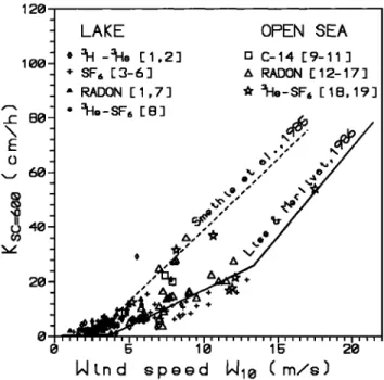
The process of air/water exchange of gases is particularly important for our understmlding of the biogeochemical cycle of environmentally active gases such as CO2, CH4, N20, dimethylsulfide, chlorofluorocarbons, etc. Most efforts have been directed toward defining a reliable relationship between the trans/br velocity K and the wind speed /4,', a key parameter in gas trm•st•r dynamics, which determines, to a large extent, the dynamic state of the air-sea boundary and the physics of gas exchange. Numerous studies have been made under various conditions including laboratory, wind tunnels of different sizes, and field experiments in lakes or the open- sea. Results/¾om the field studies are shown in Figure 1. Three distinct wave formation regions have been identified, which correspond to changes in the slope of the correlation between K and W [Liss and Merlivat, 1986]. In the first region (W <2-3 m/s), K increases only slightly with the wind speed. The second region corresponds to the occurrence of capillary waves (2-3 m/s <W <10-13 m/s), with an increased dependence of K on W. The third region, which shows
the greatest
change in K with increased
wind speed,
is
characterized by the occurrence of breaking waves and additional gas exchange through bubbles. In spite of intense efforts in determining the functional form of the transfer velocity-wind Copyright 2000 by [lie American Geophysical Union.Paper number 1999JC900088.
0148-0227/00/1999/JC900088509.00
speed relationship, the results still show large uncertainties (see re/Erences in Figure 1). Most results are bracketed by the empirical relation proposed by Liss add Merlivat [1986] on the lower side and by that ofSmethie et al. [1985] on the higher side, with no clear tendency regarding the type of experiments (laboratory, lake, or open sea) or the kind of tracer studied. In thct, we must not expect to find a strictly unique relationship, because the wind speed remains a "phenomenological" parameter that can describe only approximately the real physical and dynmnic conditions at the inter/hoe. This fact is undoubtedly one significant cause for the large scatter among the various results reported in the literature.
Nevertheless,
for practical
purposes,
good knowledge
of the
trm•s/Er velocity-wind speed correlation is of great importance for computing fluxes at a global scale and for modeling global biogeochemical cycles. With respect to the specific carbon cycle problem, aimed at assessing the fate of anthropogenic CO2 emissions, very useful data for evaluating the CO2 transfer coefficient have been obtained directly from the study of naturaland
bomb
14CO2
transfer
between
the atmosphere
and
the
ocean
[Broecker et al., 1980, 1985; Cember, 1989]. However, most measurements published to date were carried out with different
gases
(Rn, SF6,
3He) and then adapted
to CO2 using
the
theoretical relationship (1) that links the transfer coefficients of two gases K• m•d •, to their respective Schmidt numbers Sc• and Sc• (the Schmidt number is a dimensionless number defined as the ratio of the kinematic viscosity of water v to the gas molecular diffusivity D, Sc = v/D).
1 2o
1 00
._E 19o
LAKE OPEN SEA
* 31-1 -31-1. E1,2] [] C-14 1'9-11 + SF,,. [3-6] A RADON [ 12-17] ß RADON [1,7] ' al-le-SF6 E8] • . o ,._, 60
'f,
,
(.0 - • - - - / +-•-+ 0 E; 10 15 20Mind
speed
Mle (
Figure 1. Literature data tbr gas transfer versus wind speed field experiments (normalized to CO2 Schmidt number Sc=600). Lake data are froIn 1,Torgersen et al. [ 1982]; 2, diihne et al. [ 1984a]; 3, Wanni, khof et al. [1985]; 4, Wanninkhof et al. [1987]; 5, 14/a,ninM•of et al. [199 lb]; 6, Upstill-Goddard et al. [1990]; 7, Emerson et al. [1973]; and 8, Clark et al. [1995]. Open-sea data are from 9, Broecker et al. [1980]; 10, Broecker et al. [1985]; 11, Cember [1989]; 12, Broecker and Peng [1971]; 13, Peng et al. [1974]; 14, Peng et al. [1979]; 15, Kromer and Roether [1983]; 16, Sinethic et al. [1985]; 17, Glover and Reeburgh [1987]; 18, Watson et al. [ 1991 ]; and 19, Wanninkhofet al. [ 1993 ].
2. Experimental Design
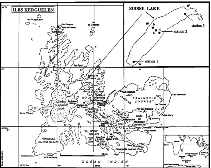
The Kerguelen Islands (Figure 2) are in the southern Indian Ocean in the 40-50 S latitude belt, where winds are usually quite strong. Lake Suisse, where the experiment was carried out, is a tYeshwater lake approximately 1 km wide and 5 km long, with a mean depth of 46.6 m 0naxi•nmn depth 9 l m), corresponding to a
volume
of 0.215 km
3 [Poisson
et al., 1990].
Owing
to the local
topography, the direction of the wind is mainly parallel to the long axis of the lake.The lake has very steep slopes, so that the potential bias in the determination of any tracer gas transfer coefficient due to shallow parts is minimized. From monitoring the water flow out of the lake, its renewal rate was esti•nated to be of the order of only 0.8% during the time of the experiment. Hence this term is neglected in the tracers' mass balance. Surface water temperature during the experiment was constant (8øC), and vertical temperature profiles also revealed a constant temperature with depth, with only a 0.09øC difference between the surface and bottom layers (z = -83 m). This indicates that the lake is thermally homogeneous and nonstratified. In the following, we shall see, however, that, in spite of this, sxnall vertical gradients in the tracer concentrations can develop during strong wind episodes. This thct is generally overlooked in most studies, and a fully homogenized tracer distribution is usually assumed. The possible effect of this slight nonho•nogeneous tracer distribution will be discussed in section 3.3.
The two tracers
(SF6 and 3He) were released
from two
aluminmn
tanks
containing
respectively,
3 m
3 of SF6
and
1 L STP
of 3He mixed
with nitrogen
to give a total
pressure
of 150 bar.
The tanks were towed in the deep layers of the lake, and the gases were released through a set of diffusing stones over 8 hours. The homogenization of the tracers in the water was then monitored atK,/r•=(Sc, 4Sc•) •n . : O
The value of the Schmidt number exponent n has been the tbcus of both theoretical and experimental s•dies. A mhew of the different theoretical results is given by Liss and Merlivat
[1986] and is summarized in Table 1. The differences in the value
of, correspond
to various
assmnptions
regarding
the bounda•
layer processes
and bounda• conditions,
•rmsponding m
different
dynmnic
s•tes of the interface,
going froin purely
diffusive to •rbulent. A number of dete•inations of thisexponent have been carried out in laborato• or field experimenB,
which are also summarized in Table 1. Both theoretical and
experimental approaches agree on the fact that the value of n tends to increase (i.e., •come less negative) when the transfer regime becomes inore energetic. The various models forec•t
values r/sing t•om -2/3 at low to -1/2 at higher regiines.
Experimental
values
follow the same trend. To compare
g•
transfer
velocities
in intermediate-
and high-wind
regimes,
they
am usually normalized to the Schmidt number of CO2 at 20øC (Sc=600) with n =-0.5. However, there is no evidence that thisvalue of the Schmidt
number
exponent
is an upper
limit and
remains construct. On the contras, expefimen•l data lWa,ninkhof et al., 1993] suggest that this value keeps on increasing (i.e., becomes less negative) for more turbulent regimes. This situation can lead m a systematic bi• in g• transfer determinations, especially for high wind speeds.To obtain new data on the g• transfer veloci•-wind speed relahonship and to gather new evidence for the variation of the Schmidt number exponent, we have carried out a dual-tracer experiment in a Kerguelen Islands lake.
Table 1. Theoretical Values of the Sch•nidt Nmnber Exponent , in Equation (1) and Literature Compilation of the Range of Variation of •t for Various Types of Experiments and Transfer Regimes Sclunidt Number Exponent n References Models -1" Whitman [1923] -2/3 • Deacon [ 1977] -0.5' Higbie [ 1935] Laboratory Experiments
-0.56 Gilhland and Sherwood [ 1934] -0.31 + 0.05 Hutchinson & Sherwood [ 1937] -0.47 Sherwood & Holloway [ 1940] -0.58 Dawson & Trass [ 1972] -0.704 Shaw & Hahfatty [ 1977] -0.41 _ 0.09 ddihne et al. [ 1979] -0.55/-0.67 Jdihne et al. [1984b] -0.45/4). 50 Ledwell [ 1984] -0.41/-0.75 ddihne et al. [1987b] -0.30•/-0.53 Wanntnkhofet al. [ 1993] Field Experiments -0.62/-0.75 a Torgersen et al. [1982] -0.505/-0.515 Watson et al. [1991] -0.35•/-0.56 Wannmkhof et al. [1993] -0.57/-0.59 Clark et al. [ 1995] -0.2•/-0.9 this work
Subscript b indicates a possible contribution of bubbles to the transfer.
• Thin film model.
• Boundary layer model.
• Surface renewal model.
a Value
was
recalculated
wifi•
Sclwnidt
numbers
from
Wanninkhof
JEAN-BAPTISTE AND POISSON: TRANSFER OF 3He AND SF6 ON A LAKE 1179
i
ILES
KERGUELEN[
SUISSE
LAKE
&
/
./ • L • •
•o•ouv•u•
•
B T
-CALO•E' •, U?U•
, .. t•m ß ••
•
%
C
OURE•
- • ....
- '2.
'
•_ •.%
• BaiZe•.t•m
de o
' • U•t R• Peri,
• • • • • ...
I I
i
I
•-•-•-•
Figure 2. Map of Lake Suisse and the Kerguelen Islands
different positions in the lake by SF6 measurements using gas chromatography equipment on the shore. After 48 hours, the tracer distribution in the lake could be considered homogeneous and monitoring the escape rate of both gases was started. SF6 and
3He samples
were
taken
at regular
intervals
at station
2a located
at the center of the lake (Figure 2) using hydrographic bottles. These samples were collected near the surface (z = -1.5 m). SF6stunpies
(and
some
additional
3He
samples)
were
also
at stations
2b m•d 2c (in the middle of the lake) and at stations 1 and 3 at both ends of the lake (Figure 2) to monitor the overall homogeneity of the tracer distribution. Wind speeds were recorded at a height of 4 m at three different positions on the shore (indicated by the letter W in Figure 2). The tilne-series of the three anemometers are in good agreement, with differences not exceeding 10%. For relating gas transfer to wind speed, raw wind speeds were converted to the standard wind speed W10 at 10 m height following Large and Pond [1981], leading to a correction factor of around 1.10. SF6 samples were analyzed in a container laboratory installed on the shore using the same technique as described by Wanninkhof et al. [199 l a]. Analytical precision was within _+1% (1 o error). Helium samples were taken in copper tubes and returned to the laboratory at Saclay for helium extraction m•d mass spectrometric measurement using our
standard procedure [Jean-Baptiste et al., 1992] for oceanic
samples.
Note that since
the 4He concentration
is at its natural
background
and
is essentially
constant,
the 3He
concentrations
are
expressed
as
an isotopic
ratio
R=3He/4He
using
the
delta
notation:
$3He(%)=
(R/Ra-1)x
100
where Ra is the atmospheric helium isotopic ratio. The overall
relative
uncertainty
in the 3He/4He
ratio,
AR/R
is less
than
0.5%
(l o error).
3. Tracers Results and Gas Transfer
Velocity/Wind Speed Relationship
SF6
and 3He time-series
at station
2a, located
at the center
of
the lake, are displayed in Figure 3 along with the record of thewind
speed.
Both
3He
and
SF6
records
show
a steady
decrease
of
the tracer concentration due to gas escape to the atmosphere. Over the 30 days of available SF6 measurements at station 2a, SF6
concentrations
were
divided
by 3.7. During
the same
period,
3He
concentrations were reduced even more rapidly, by a factor of6.7, as expected
from the greater
diffusivity
of 3He.
The plot of
the logarithm of the tracers concentrations versus time (Figure 4) shows that the decay of both tracers is exponential.
velocities versus •nean wind speeds, as we shall see in section 3.2
when using
the second
•nethod.
For each tracer,
the (z and
coefficients are adjusted by solving the tracer •nass balanceequation
(equations
(2a) and
(2b) for SF6
and
3He,
respectively)
for the lake between fi•ne t and t+dt, with surface tracer fluxes
forced by the •neasured wind speed (see (3a) and (3b)), so as to
•nini•nize
the •nis•natch
between
the calculated
b3He(t)
and
CsF6(t) curves and the data. This mis•natch is defined as the squared distance between the •neasured concentrations and thecalculated curve.
38
•'SF6(t+dt) = CSF6(t) - (I)sF6(t)xdt/h (2a)
Et
•3He(t+dt)
=/53He(t)
- rI)3,e(t)xdt/h (2b)
•'
where
h is
•nean
depth
and
with
(I)sF6(t)
= [3SF6
[/Vt•F6
[CSF6(t)
- Ceq.]
(3a)
•' •, with Ceq = 0.
(I)3He(t)
= •33HeVg
'ram
[b3He(t)
- beq.]
(3b)
with &q.=
-1.6% [Weiss,
1970; Top et al., 1987].
"'g'"•"il•'i•'i•4'ilg'iU'•'•'•:4'flg'•'•'-•'5•'Sg'•i
In the applicable
range
of wind
speeds
(0-10 •n/s),
this
best
fit
4 6 0 10 12 14 16 18 2• 22 24 26 28 :•'32 34 3• 38 days afLer Ln JecLLon
Figure
3. (a)
Decline
of
SF6
concentration
and
(b)
excess
3He
($ He%) with ti•ne, (c) •nean wind speed corrected to 10 •n, W•0.The solid
line for SF6
and fi3He
is the best
fit of the data
using
a
power law K=I3 W •, with tz = 1.5 (see section 3.1), and the dashed lines correspond to tz = 1.3 and 1.7From these time-series, we calculate the gas transfer velocities versus wind speed in two different ways. First (section 3.1), we assrune that this relationship cm• be well represented by a power law, K = 13W•0, where K is transfer velocity and W•0 is wind speed at 10 •n height, and we fit the parmneters tz and [3 to our experimental data. The second •nethod (section 3.2) si•nply consists of calculating the mean transfer velocity, according to (4), m•d the •nean wind speed for each successive data point.
In the following, both •nethods are explained, with their
respective
advantages
and !i•nitations,
and their results are
co•npared.
Then, we look at the potential
effect of even slight
vertical heterogeneities in the tracers' concentrations on the detemfination of the gas transtar velocities.3.1. Determination of a Functional Form K = 13 •
For the sake of si•nplicity, we first assrune that the gas transfer velocity versus wind speed relationship can be represented by a power law', K = [3 W • .This choice sea,ns reasonable to us in light of the available data in the literature, which indeed display this type of behavior. Moreover, this •nethod avoids the proble•n of the nonlinearity bias that arises when calculating mean transfer
procedure leads to tz •1.5 for both gases, [3sF6=0.71_-t-0.06 and [33,•=1.8_--t-0.1 (for K in cm/h and W•0 in •n/s). The quality of the fit is only a weak function of the exponent tz in the range 1.3-1.7 as shown in Figure 3 where the dashed lines, representing the best fit curves for tz --1.3 and 1.7, are ahnost indistinguishable frown the solid curve (corresponding to tz =1.5). This value tz •1.5_--t-0.2 co•npares well with the 1.64 exponent value derived by Wanninkhofet al. (1991 b] from a lake experi•nent using SF6.
Our results correspond to a •nean Sch•nidt nmnber exponent of -0.43_+0.1 for the coinplate experi•nent, with Schmidt numbers for
3He
and SF6
of 219 and 1912, respectively
[d•hne
et al., 1987a;
King and Saltzman, 1995]. In Figure 5, the gas transfer velocity/wind speed relationships for both tracers are normalized to CO2 at 20øC (Sc=600) using a Sch•nidt nmnber exponent n=- 0.5, as is usually done in the literature for co•nparison purposes.E3 - O 4• 2 : - - : - [] O O 20 30
cl•y•
•'Ften
Ln Ject
Lon
F)gure
4. Logarithm
of the tracers'
concentrations
(SF6
and
JEAN-BAPTISTE AND POISSON: TRANSFER OF 3He AND SF6 ON A LAKE 1181 •O L 40
0 30
',0 20
•0 •0 40 10- [] D D 0 2 4 6 B 10• tnd speed
L*l•e (m/s)
Figure 5. Transfer velocity, normalized to CO2 (Sc=600) using a constant Schmidt number exponent n=-0.5, plotted against wind speed W•0. Curves labeled 1 and 2 are the present results for SF6and 3He, respectively.
LM and S85 stand
for the Liss and
•[erlivat [1986] and $methie et al. [1985] relationships,respectively.
The two open squares
are global
•4C transfer
coefficients from Broecker et al. [1985] and Cember [1989]. The solid stars are the dual-tracer results of Watson et al. [1991] and the open stars are from Wanninkhofet al. [1993] and Clark et al. [1995].
In the Lake Suisse
experiment,
the curves
deduced
from •He and
SF6 significantly disagree with those from Liss and Merlivat[1986]. To show the practical
consequences
of this large
mismatch,
we display
the $•He time -series
that would result
t¾om
the Liss and Merlivat [1986] (LM) relationship
(applied
to
-•He
using
the
exponent
n =-0.5)
in Figure
6. The
LM relationship
underestimates
the •He mean
evasion
rate
actually
deduced
from
the present
experiment
by 40% (a figure
that corresponds
to the
factor that must be applied
to the •He transfer
coefficient
K3,e=l.8xW •'s to fit the curve calculated with the LM correlation in Figure 6).Our results
are on the higher
side
of the literature
data.
They
are consistent
with the gas transfer
velocities
derived
from •4C
1
0'
18 12 14 26 28 3lB 32 34 36 38
deye eldLoP In Jeer, ton
Figure
6. Computed
$•He ti•ne
-series
that
would
result
from
the
use of the Liss and Merlivat [1986] relationship (solid line) andco•nparison
with
the
measured
$•He
(squares).
4 6 8
speed
L.l•e (m/s)
lO a aa••
a
a•P a aa a a•m
•1
aa
a D a a i i i i i i i i i i I I I I I I I I I I III I I I I I I Istgma(Mtj)
Figure
7. (a) Comparison,
for •He, between
the
Ku-W
u couples
(open squares) calculated from equation (4) m•d the power law
• 15
K,•ue:l.8xW determined in section 3.1. The (i,j) couples used
tbr calculating
K u were
selected
along
the $•He(t)
best
fit curve
computed from (2b) and (3b) (wellqnixed box model) using the
law K3.•=I.8xW
•'s. The difference
between
the solid curve
(representing
K=I.8xW
•'s ) and the open
squares
is due to the
non-linearity bias. (b) Bias shown as an increasing function of the wind speed variability, expressed as the sig•na of the wind speed distribution (cry) between ti•nes t• and tj.oceanic inventories, which appear to be among the most robust field determinations because they represent global long-term averages. They are also in good agreement with the results of
Wam•inkhof
et al. [ 1993]
obtained
with the •mne
tracer
pair
(3He
and SF6) on Georges Bank. For low wind speeds, the present
results
tend
to be slightly
above
Clark et al.'s [1995] recent
•He-
SF6 data (Figure 5).3.2. Individual Kt/Determinations
For each gas, a mean transfer velocity Ke and a mean wind speed W e can be computed for two successive measurements at times ti and tj respectively, by the standard equation:
Ke=h/(tj-t3 [ln (Ci-Ceq)/(Cj-Cm) ] (4)
where Ci and Ci are the measured concentrations (for SF6) and the
measured
$3He(%)
(for helium)
at times
h and
t•, respectively,
and h is the •nean depth of the lake (h=46.6 •n). The suscript "eq"
30 0 2 4 6 B 10
• In d speed
1,410
(m/s)
20 o oFigure 8. Calculated K values versus incan wind speed for every
possible
pair
of (a) 53He
and (b) SF6
measurements.
(The t•w
negative values of K, due to some negative values of the tracer
concentration
difference
CrCj , were eliminated
because
they are
physically •neaningless.) Open squares denote K values calculated from adjacent data points. For each tracer, the power law K = 13H•0 determined using method 1 is included for comparison. lOO ,• ,,•__ =mt, m. 1•'•
A
ßt.e.
2".
'•,q,
+ ot,
e .3
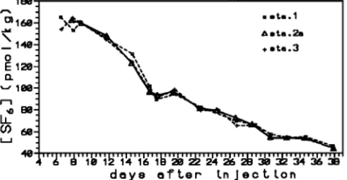
ß "'/,'' '•'' • •' { •' { •J' • •;' { I• "• '• '•,•; '• '• '• '• 'õ•; '52 '• deye e•'ter In Jec t ton Figure 9. Comparison of SF6 surface concentrations measured atstations 1,2a, and 3.
denotes the tracer background at equilibrium with the
atmosphere:
Ceq.=0
for SF6
and
153Heeq
m-1.6%
[Weiss,
1970;
Top
et al., 1987]. In fact, there is no theoretical reason to restrict this calculation to consecutive data points only, and the method can be extended to every possible pair of measurements Ci and C• at
times
t• and t•, with K,• being
the •nean
transfer
velocity
averaged
over the time period tœt• and W• the mean wind speed over the same period. The main drawback of this method is the bias in the determination of the transfer velocity/wind speed relationship owing to its nonlinear nature; that is, K/• does not equal K(Wi•). This bias is clearly noticeable on the example displayed in Figure 7a; here the squares represent all the K/• versus W/• pairsdetermined
fi'om fictive
$3He data points
selected
at a 1-day
tYequency
on the theoretical
curve $3He(t)
of section
3.1
computed
using
the power
law K(cm/h)=l.8xW
1.5.
The solid
curve
is the power
law K(cm/h)=l.8xW
1.5.
If there
was
no bias,
the points would lie exactly on the curve. Figure 7b shows that, as expected, the bias is indeed a growing function of the sigma of the wind speed distribution (c•u) between ti•ne t• and tj, with bias up to 20% tbr episodes of higher wind variability.
Figures 8a and 8b display all possible K o versus mean wind
speed
W
e pairs
deduced
frown
our
3He
and
SF6
measurements
(the
open squares denote K,• corresponding to successive measurements) and compare the results to the functional forms K
= [3
W 15 obtained
in section
3.1. In addition
to the nonlinearity
bias discussed above, this second method clearly leads to a largescatter
in the K,• determinations
(note that this scatter
is not
reduced when selecting only successive measurements). For these two reasons, we thvor the first approach (method 1) which avoids the nonlinearity problem and s•nooths out the experimental scatter. In the following section, we examine the possible effects of s•nall heterogeneities in the vertical distribution of the tracers and show that •nuch of the scatter in the /•;• determination is indeed related to these heterogeneities.3.3. Heterogeneity Effects
Ahnost all of the studies published to-date assume a well- lnixed reservoir. Vertical mixing is assumed to be efficient enough to ensure a homogeneous vertical tracer distribution. Possible horizontal heterogeneities effects due, for instance, to the occurrence of shallow parts, m-e also ignored. In the present
experiment,
unlike
$3He
•neasurements
which
were
mostly
made
in the sur/hce layer at one central station, a number of SF6 stunpies were taken at different depths at every station indicated in Figure 2 to monitor the degree of homogeneity of the lake. This •nonitoring shows (Figure 9) that there is no horizontal tracer gradient. However, the SF, water column profiles show
JEAN-BAPTISTE
AND POISSON:
TRANSFER
OF 3He
AND SFo
ON A LAKE
1183
1.3• see•,
A
-
days
•1 1
•,
•.
B
.-.
,.,
.
1•'1 • ...
•,, ,
•1•,
deys e•ter
In Ject ton
m •,
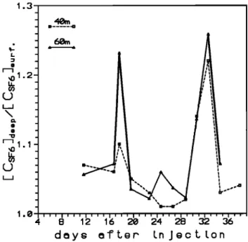
•i•ure •0. Time -series at station 2a of the ratio bc•ccnmeasured
S• concentrations
at lake
dccp
waters
(at
dopes
z=-60
'" '•' "•' '•'• '• '•'• '•'•'•
'•'•'•'•
'• '•'•
and
•O m) and
at suffacc
watcrs.
dmy• m•Ler In JecLlon
that SF6 concentrations in the deep layers sometimes tend to be significantly higher than surface concentrations (Figure 10), hence leading to some heterogeneity in the tracer vertical distribution. This means that although the convective mixing of the lake is rapid owing to the lack of stratification, it is not instantaneous. Hence it takes some time for the surface layer to be msupplied with the tracers from deeper layers, especially during high wind episodes. In the following, we look at the consequences of this phenomenon on the determination of the gas transfer velocity. Instead of assuming a well-mixed reservoir, we consider a vertical diffusivity Dv of the tracer in water. The vertical distribution of SF6 versus time is computed using a 20- layer &fiBsion model developed for this study. At each time step, the tracer fluxes exchanged between each layer (with a constant thic'kness dz=h/20) and its neighbors are computed using Fick's law (equations 5a and 5b) mid the tracer concentration in each layer is then cmnputed from the mass balance equation (6).
F,.,+•(0 = -Dv[C,(t) - C,+•(0]/dz (5a) where F,,,+•(t) is the flux between layer i and i+ 1, with
Fbottom
= 0, Fsurf
= •3W
"5
[C,•(t)-Cm.]
(5b)
C,(t+dt) = Ci(t)+dt/dz [F•,i+•(0 - Fi, i-•(O] (6) In addition to the parameters or and [3, which are adjusted as in section 3.1 to minimize the mismatch between the experimental data and the calculated SF6(t) curve for the surface layer, the diffusivity D• is also tuned simultaneously so as to reproduce the range of observed vertical concentration gradients between surface and deep SF6 concentrations shown in Figure 10. Our best
estimate
of the vertical
diffusion
coefficient
is D• • 50 cm2/s.
This
value is on the higher side of vertical diffusivities observed in nature [Broecker and Peng, 1982], which is consistent with a lionstratified lake. Although the computed time evolution of the surface concentration is more "wavy" (Figure 11), as expected tYmn a physical point of view, the coefficients of the power lawFigure
11. Best
fit curve
(solid
line)
of the
(a) 153He
and
(b) SF6
measured surface concentration time -series using the vertical diffusion model. The dashed line is the best fit curve with the well-mixed box model (see Figure 3) and is included here for co•nparison.
Ksv6 = •3• remain basically unchanged, thereby fully justifying the homogeneity assumption used in method 1.
However, if method 2 is used, the consequences are important: Figure 12 is identical to Figure 7a, but this time the theoretical
curve
b3He(t)
is the concentration
in the surface
layer
of the 20-
layer diflhsion model instead of the concentration calculated with-- o
40--
-"*,, ,,
- 0 " !20
..•.
'..
'T' ".-
.
•0"
10 " ." _ o , ", 0 2 4 6 B 10• Lnd epeed
•o
Figure 12. Same as Figure ?a, but using the vertical dieusion model instead of the well-mixed box model. Note the much larger
the well-mixed reservoir model. It shows that the fluctuations in
the tracer's surface layer concentration have a large effect upon
the scatter
of the KO. This marked
effect
could
be a significant
cause of discrepancy mnong the experi•nental gas exchange coefficients reported in the literature, most of which are indeedbased on the use of method 2.
This fact is an additional strong argument in favor of the first method tbr determining the gas transfer velocity/wind speed
relationship
(i.e., the use of a prescribed
functional
form), as it
avoids both nonlinearity bias and excessive dispersion caused bythe experimental
scatter
of the data and, more important,
by any
possible
departure
(even modest)
frmn the well-mixed
reservoir
conditions.
4. KsF6
- K3ne
Relationship
and Schmidt Number
Exponent n
To experimentally determine the Schmidt number exponent in
(1), the mean
3He
and
SF6
transfer
velocities
K/• are
computed,
as
in section 3.2, for every possible pair of tneasurements Ci and C•
at times
ti and
t• using
(4). Since
SFo
and
3He
were
not
collected
at exactly
the same
time, the 3He data
are extrapolated
to the
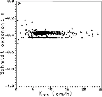
corresponding SFo sampling time. This extrapolation is done using the transfer velocity versus wind speed relationship of section 3.1, the measured wind speed, and the tracer mass balance equation. Figure 13 shows the relationship between the Schmidt
number
exponent
n in (1) and
KsF•,
ß The SF6
and
3He
Schmidt
numbers are taken from King and Saltzman [1995] and diihne et al. [1987a], respectively. The error bars are derived from the
analytical
errors
in SF•,
mad
3He measurements
and also
from
the
uncertainty quoted in the literature (_+5%)in the determination ofthe Schmidt numbers. Note that the error zLK in the transfer
coefficient varies as the reciprocal of the time interval (trt•), so
that K• values
calculated
frmn large time intervals
are more
accurate. The general trend shown in Figure 13 is consistent with our current understanding of gas transfer at water-air interface.0.0 0-0.4 g_ X .0-0.6
t--O.
o -1.0 O 5 10 15 20 25KSF6 ( C m/h)
Figure 13. Trend of the Schmidt number exponent versus SF6 transfer velocity (KsF6) deduced from our experiment. The mean KsFo value for the complete experiment and the average Schmidt number exponent derived from the best fit of the data using
K=I3
•4
•'q are
also
included
(dashed
lines).
0.0 -0.4- - . . -0.6 - - -0.8 _ on •11, I I jffi [] • O 0 [] . - - -• .0
I I I I I I I I I•1 I I I I I I !
I I I I I I I
I I I I I I I
I I I I I I I
computed with the wellqnixed box model (open squares) and the vertical diffusion model (crosses).
For low transfer regi•nes, the n exponent is in the range [-1, -2/3] and of the order of -0.5 for intermediate regimes, in agreement with the theory. For higher transfer regimes, however, the value of n keeps increasing and reaches values close to -0.2, possibly owing to the contribution of bubbles to the gas transfer (see discussion below). To check that this trend is not an artifact due to the slight vertical heterogeneity, we compared (Figure 14) the Schmidt number exponent n calculated assuming a well-mixed reservoir (infinite vertical •nixing rate) to that calculated for a
finite vertical
•nixing
(with D•=50 cm2/s).
In Figure
14, the
squares represent the n values corresponding to all (K/•)sr6 and
(K,•)3,•
pairs
determined
from
fictive
b3He
data
points
selected
at
a l-day
frequency
on the theoretical
curve
b3He(t)
and
Csr6(t)
of
section 3.1 (wellqnixed boxqnodel)computed using the powerlaw K3He-=I.8xW
•'5.and
KsFo=0.71xW
•.5 The crosses
represent
the same type of calculation but this time using the vertical diffusion box-model. A cmnparison between the two sets of results shows that ta'king into account the vertical heterogeneity shifts the average value of n by 0.05 (-0.38 instead of-0.43) and adds significant scatter to the results. This scatter appears to be greater tbr low transfer regimes, with a trend to higher n, i.e., the opposite of what is shown in Figure 13. For intermediate- and high- transfer regimes, there is no global effect on the trend of the n exponent versus the transfer regime. This strongly suggests that the experimental trend between , mad KsF• observed in our experiment (Figure 13) is not an artifact due to the finite rate of vertical mixing but a genuine phenomenon.
This expemnental result supports earlier data of Wanninkhofet al. [1993] which show an increase in the apparent Schmidt number exponent with increasing transfer regime (that is, it beco•nes less negative). Beyond the n=-0.5 value predicted by the models, this increasing trend was interpreted by the authors as the contribution of bubbles to the gas transfer. In this case, the transtar coefficient K'i for a gas i at any given wind speed can be rewritten as the su•n of two co•nponents Ki and K•i.
JEAN-BAPTISTE
AND POISSON:
TRANSFER
OF 3He
AND SF6
ON A LAKE
1185
0.0 •-0.4 X -O-0.6 o -1.0 /02 31-1./SF,,. 3He/02 3He/At'=He
0.0 1.0 2.0 3.0 4.0 E;.0Kbj/Kj
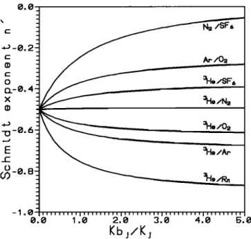
Figure 15. Theoretical variation of the apparent Schmidt number
exponent
n' versus
K•,/K•
derived
from
equation
(8) for various
inert
gas
pairs
(i,j). The Kb//Kbj ratios
have
been computed
assuming
that
K• varies
with the gas
solubihty
and
diffusivity
as (SRT)ø'3
D
(where
SRT is the Ostwald
solubility
coefficient)
[Keeling,
1993].
Gas solubilities and diffusivities are computed using the polynomial fit of Wanninkhof[ 1992] for freshwater at 8øC.where Ki is the "normal" gas transfer coefficient and K•i is the contribution due to bubbles. In a dual-tracer experiment, the variable Schmidt number exponent n' which is inferred from the tracer measurements will be linked to the normal n exponent (without gas transfer through bubbles) by the following equation:
x',/x) =( x, +
+
(Sc,/Sc)" (8)
Giving
ln[(Sc,/Sc,)
n
+ (K•,/K•j)(Kb,
/ K•.)]/(1
+ K•,
/ K•.)]
(9)In(Sq.
/ Scj)
where
Kt,j / K• represents
the ratio of the bubble-mediated
gas
trm•sfer to the normal air-sea transfer and Kt,,/Kt,j is the ratio of the transfer coefficients through bubbles for the two species. Weverify
with (9) that if K0j/K• --> 0 (no bubble
contribution
to the
transtar), then n '--> n, and, on the other hand, if Kbj / K• --> c• (gastransfer
largely
dominated
by the bubbles),
then n '--> ln(Ko//
K•j)/ln(Sc•/Scs)
(equation
(10)).
In the general
case,
(10) shows
us
that n' values will depend on the relative efficiency of the bubble mediated transfer (Ko/K) of each species i and j and that n' will
be larger
or smaller
than
n, depending
on the value
of the ratio
rbi
/ K•s relative
to (Sci /Scj)"(Figure
15). Bubble-induced
gas
exchange in general depends both on the gas diffusivity and
solubility,
with larger effects
for gases
with lower solubility
[Merlivat and Memery, 1983]. Keeling [1993] suggested that the bubble-induced gas transfer component Ko should scale as (SRT)-0.3
D0.3s
(where
SRT is Ostwald
solubility
coefficient).
Because
the solubilities of helimn and SF6 are quite similar [Ashton et al.,1968; Weiss, 1971 ], the Kb3ue / Kt, sF6 ratio will be of the order of
(SC3H
e /SCsF6)
'0'35
(• 2.13 at 8øC).
As this
value
is below
(Sc3,e
/SCsF6)
-ø'5 (= 2.95 at 8øC), the Schmidt
number
exponent
n'
should increase relative to n, with an asymptote at n '=-0.35 after (9). This prediction is in apparent agreement with our experimental findings (Figure 13). This agreement could also be tbrtuitous, however, as it requires a rather large contribution of the bubbles to gas transfer, which is not expected here, considering wind speeds recorded during the experiment. This interpretation of the variation of the Schmidt number exponent based on the influence of bubbles would need to be tested against different gas pairs, especially those with large solubility differences, in order to be fully validated. Therefore the variation of the Schmidt nu•nber exponent observed here and its relatively low mean value for the complete experiment are facts, already observed by others (Table 1), whose explanation still requires
further clarification.
5-Conclusion
The SFd3He
deliberately
released
tracer
method
in a large
freshwater lake of the Kerguelen Islands allowed the determination of both gas transfer velocities in a wind speed
range
of 0 to 10 •n/s,
by monitoring
SFo
and
3He
escape
rates
over
a month. h• this experiment, the Liss and Merlivat [1986] relationship underestimates the actual gas transfer rate by about 40%. The present results fall in the range of transfer velocities tbund in most recent experiments [Wanninkhofet al., 1993] and
also
agree
with oceanic
14CO
2 inventories.
Comparison
of Ksvo
and K3}• shows, as expected, m• increasing trend of the Schmidt number exponent (that is, it becomes less negative) with increasing transfer velocities, but with values extending beyond the n = -0.5 coefficient usually employed for normalizing gas transfer data to CO2. This raises the problem, discussed previously by different authors and still open to question, of the validity of the normalization methods used to calculate Kco2 from gas transfer experiments, especially in high-wind regimes, and points to the need for further clarification of the Schmidt relationship in gas transfer experiments.
Acknowledgements. The KERLAC project was supported by the Ten'itoires des Terres Australes et Antarctiques Fran9aises (TAAF). We
are deeply grateful to A. Lamalle, who supervised with great
professionalism the logistics of the project on the Kerguelen Islands. We
thank C. Brunet and P. Hegesippe, who took part in the lake survey, and A. L'Huillier and C. Lemarchand, who actively participated in the Suisse
Lake experiment.
References
Ashton, J. T., R. A. Dawe, K. W. Miller, E.B.Smith, and B.J. Stickings, The solubility of certain gaseous compounds in water, J. Chern. Soc.,
A, 1793-1796, 1968.
Broecker, W. S., and T. H. Peng, The vertical distribution of Radon in the
Bomex area, Earth Planet. Sci. Lett., l l, 99-108, 1971.
Broecker, W. S., and T. H. Peng, Tracers in the Sea, 690 pp., Lainont-
Doherty Earth Observatory, Palisades, N.Y., 1982.
Broecker, W. S., T. H. Peng, G. Mathieu, R. Hesllein and T. Torgersen, Gas exchange rate measurements in natural systems, Radiocarbon, 22,
676-683• 1980.
Broecker, W. S., T. H. Peng, G. Ostlund and M. Stuiver, The distribution
of bomb radiocarbon in the ocean, d. Geophys. Res., 90, 6953-6970, 1985.
('ember, R., Bomb radiocarbon in the Red Sea: a medium-scale gas
exchange experiment, d. Geophys. Res., 94, 2111-2123, 1989.
Clark, J. F., P. Sclfiosser, R. Wanninkhof, H. J. Simpson, W. S. F. Schuster, and D. T. Ho, Gas transfer velocities for SF6 and 3He in a small pond at low wind speeds, Geophys. Res. Lett., 22, 93-96, 1995.
Dawson, D. A., and O. Trass, Mass transfer at rough surfaces, Int. d. Heat Mass Transfer, 15,1317-1336, 1972.
Deacon, E. L., Gas transfer to and across an air-water interface, Tellus,
Emerson, S., W. S. Broecker, and D. W. Schindler, Gas-exchange rate in a small lake as determined by the Radon method, J. Fish. Res. Board
Can., 30, 1475-1484, 1973.
Gilliland, E. R., and T. K. Sherwood, Diffusion of vapors into air streams,
Ind. Eng. Chem., 26, 516-523, 1934.
Glover, D. M., and W. S. Reeburgh, Radon-222 and Radium-226 in southeastern Bering Sea shelf waters and sediment, Cont. Shelf Res., 5,
433-456, 1987.
Higbie, R., The rate of absorption of a pure into a still liquid during short
periods of exposure, Trans. Am. Inst. Chem. Eng., 35, 365-369, 1935.
Hutchinson, M. H., and T. K. Sherwood, Liquid film in gas absorption,
Ind. Eng. Chem., 29, 836-840, 1937.
J'fihne, B., K. O. Munnich, and U. Siegenthaler, Measurements of gas
exchange and momentum transfer in a circular wind-water tunnel, Tellus, 31,321-329, 1979.
J:41me, B., K. H. Fischer, J. Ilmberger, P. Libner, W. Weiss, D. Imboden,
U. Lemnin, and J. M. Jaquet, Parametrization of air/lake gas exchange,
in Gas' Transfer at Water Surfaces, edited by W. Brutsaert and G. H. Jirka, pp. 459-466, D. Reidel, Norwell, Mass., 1984a.
J'filme, B., W. Huber, A. Dutzi, T. Wais, and J. Ilmberger, Wind/wave- tunnel experiment on the Schmidt number and wave field dependence of air/water gas exchange, in Gas' Transfer at Water Surfaces, edited by W. Brutsaegt and G. H. Jirka, pp. 303-309, D. Reidel, Norwell,
Mass., 1984b.
J'glme, B., G. Heinz, and W. Dietrich, Measurement of diffusion coefficients of sparingly soluble gases in water with a modified Barrer method, J. Geephys. Res., 92, 10,767-10,776, 1987a.
J'glme, B., K., O. Munnich, R. B osinger, A. Dutzi, W. Huber, and P.
Libner, On parameters influencing air-water gas exchange, J.
Geephys. Res., 92, 1937-1949, 1987b.
Jean-Baptiste, P., F. Mantisi, A. Dapoigny, and M. Stievenard, Design and performance of a mass spectrometric facility for measuring helium isotopes in natm'al waters and for low-level tritium determination by
the
3He
ingrowth
method,
Appl.
Radtat.
Isot.,
43,
881-891,
1992.
Keeling, R. F., On the role of large bubbles in the air-sea exchange and
supersaturation in the ocean, J. Mar. Res., 51,237-271, 1993.
King, D. B., and E. S. Saltzman, Measurement of the diffusion coefficient of sulfur hexafluoride in water, d. Geephys. Res., 100, 7083-7088,
1995.
Kromer, B., and W. Roether, Field measurements of air-sea gas exchange by the Radon deficit method during JASIN 1978 and FGGE 1979,
J9Ieteor Forschungergeb., A/B, 24, 55-75, 1983.
Large, W. P., and S. Pond, Open ocean momentum flux measurements in moderate to strong winds, J. Phys. Oceanogr., 11, 324-336, 1981.
Ledwell, J. J., The variation of the gas transfer coefficient with molecular diffusivity, in Gas' Transfer at Water Surfaces, edited by W. Brutsaert
and G. H. Jirka, pp. 293-302, D. Reidel, Norwell, Mass., 1984.
Liss, P.S., and L. Merlivat, Air-sea gas exchange rates: introduction and synthesis, in The Role of Air-Sea Exchange in Geochemical Cycling, edited by P. Buat-Menard, pp. 113-127, D. Reidel, Norwell, Mass., 1986.
Merlivat, L., and L. Memery, Gas exchange across an air-water interface: experinmntal results and modeling of bubble contribution to transfer.
•. Geephys. Res., 88, 707-724, 1983.
Peng, T. H., T. Takahashi, and W. S. Broecker, Sin-face Radon
measurements in the north Pacific ocean station Papa, d. Geephys.
Res'., 79, 1772-1780, 1974.
Peng, T. H., W S. broecker, G. G. Maflfieu, and Y. H. Li, Radon evasion
rates in the Atlantic and Pacific oceans as detem•ined durinb
Geesecs program, J. Geephys. Res., 84, 2471-2486, 1979.
Poisson, A., C. Brunet, and P. Hegesippe, Le lac Suisse, archipel des iles Kerguelen: Bathymatrie et hydrologic, report, 55 pp., Ten'es Austr. et
Antarct. Ft., Paris, 1990.
Shaw, D. A., and T. J. Hahfatty, Turbulent mass transfer rates to a wall
for large Schmidt numbers, AIChE d., 23, 28-37, 1977.
Sherwood, T. K., and F. A. Holloway, Performance of packed towers-
liquid film data for several packings, Trans. Am. Inst. Chem. Eng., 36,
3 9-70, 1940.
Smethie, W. M., T. T. Takahashi, D. W. Chipman, and J. R. Ledwell, Gas exchange and CO2 flux in the tropical Atlantic Ocean determined from
222Rn and pCO 2 measurements, d. Geephys. Res., 90, 7005-7022,
1985.
Top, Z., W. C. Eismont, and W. B. Clarke, Helium isotope effect and
solubility of helium and neon in distilled water and seawater, Deep - Sca Res., PartA, 34, 1139-1148, 1987.
Torgersen, T., G. Matlfieu, R. H. Hesslein, and W. S. Broecker, Gas exchange dependency on diffusion coefficient: direct 222Rn and •He comparisons in a small lake, d. Geephys. Res'., 87, 546-556, 1982. Upstill-Goddard, R. C., A. J. Watson, P. Liss, and M. I. Liddicoat, Gas
transfer velocities in lakes measured with SF6, Tellus, ser. B, 42, 364-
377, 1990.
Wmminkhof• R., Relationship between wind speed and gas exchange over the ocean, d. Geephys. Res.. 97, 7373-7382, 1992.
Wamfinkhof} R., J. R. Ledwell, and W. S. Broecker, Gas exchange-Wind
speed relation measured with sulfur hexafluoride on a lake, Science,
227, 1224-1226, 1985.
Wanninkhof, R., J. R. Ledwell, and W. S. Broecker, Gas exchange on
Mono Lake and Crowley Lake, California, d. Geephys. Res., 92,
14,567-14,580, 1987.
Wanninkhof, R., J. R. Ledwell, ,and A. J. Watson, Analysis of sulfur
hexafluoride in seawater, d. Geephys. Res'., 96, 8733-8740, 1991a.
Wamfi•fidmf, R., J. R. Ledwell, and J. Crucius, Gas transfer velocities on lakes me,xsured with sulfur hexafluoride, in Proceedmgs of the Second
b•ternat•onal Syruposram on Ga•' Tramfer at Water Surfaces', edited by S.C. Wilhems and J. S. Gulliver, pp. 441-458, Am. See. of Civil
Eng., New York, 1991b.
Wanninkhof, R., W. Asher, R. Weppemig, H. Chen, P. Schlosser, C.
Langdon, and R. Sambrotto, Gas transfer experiment on Georges Bank using two volatile deliberate tracers, d. Geephys. Res'.. 98, 20,237- 20,248, 1993.
Watson, A. J., R. C. Upstill-Goddard, and P. S. Liss, Air-sea gas
exchange in rough and stormy seas measured by a dual-tracer
technique, Nature, 349, 145-147, 1991.
Weiss, R. F., Helium isotope effect in solution in water and seawater,
Science. 168, 247-248, 1970.
Weiss, R. F., Solubility of helium and neon in water and seawater, d.
Chem. Eng. Data, 16, 235-241, 1971.
Whitman, W. G., The two-film theory of gas absorption, Chem. Metal. Eng., 29, 146-148, 1923.
P. Jean-Baptiste, Laboratoire des Sciences du Climat et de
l'Environnen•enk CEA/CNRS, Centre d'atudes de Saclay, F-91191 Gif- sur-Yvette Cedex• France. (pjb(•_ ]sce.saclay. cea.fr)
A. Poisson, Laboratoire de Physique et Chimie Marines, CNRS/UPMC,
4 place Jussietk boite 134• F-75252 Paris Cedex 05, France. (Received June 17, 1996: revised October 28, 1998: accepted January 2, 1999).

![Figure 6. Computed $•He ti•ne -series that would result from the use of the Liss and Merlivat [1986] relationship (solid line) and co•nparison with the measured $•He (squares)](https://thumb-eu.123doks.com/thumbv2/123doknet/14784636.598162/6.894.77.444.101.448/figure-computed-series-merlivat-relationship-nparison-measured-squares.webp)