Applications of robust optimization to queueing and inventory systems

Applications of Robust Optimization to Queueing and

MASSACHUSETTS INSTITUTE

Inventory Systems

OF TECHNOLOGY

by

_AUG

₀

_{1 2011}

Alexander Anatolyevich Rikun

LIBRARIES Submitted to the Sloan School of Management ~~~~

in partial fulfillment of the requirements for the degree of Doctor of Philosophy in Operations Research

at the

MASSACHUSETTS INSTITUTE OF TECHNOLOGY

June 2011

@

Massachusetts Institute of Technology 2011. All rights reserved.

J" /

A uthor ... _{... .. ... . .}

Sloan School ment

16, 2011

Certified by ...

Dimitris Bertsimas Boeing Professor of Operations Research Co-Director, Operations Research Center Thesis Supervisor

C ertified by ...

David Gamarnik

Associate Professor of Operations Research Thesis Supervisor Accepted by...

Dugald C. Jackson

Patrick Jaillet Professor, Department of Electrical Engineering and

Computer Science Co-Director, Operations Research Center

Applications of Robust Optimization to Queueing and Inventory

Systems

by

Alexander Anatolyevich Rikun

Submitted to the Sloan School of Management on May 16, 2011, in partial fulfillment of the

requirements for the degree of

Doctor of Philosophy in Operations Research

Abstract

This thesis investigates the application of robust optimization in the performance analysis of queueing and inventory systems.

In the first part of the thesis, we propose a new approach for performance analysis of queueing systems based on robust optimization. We first derive explicit upper bounds on performance for tandem single class, multiclass single server, and single class multiserver queueing systems by solving appropriate robust optimization problems. We then show that these bounds derived by solving deterministic optimization problems translate to upper bounds on the expected steady-state performance for a variety of widely used performance measures such as waiting times and queue lengths. Additionally, these explicit bounds agree qualitatively with known results.

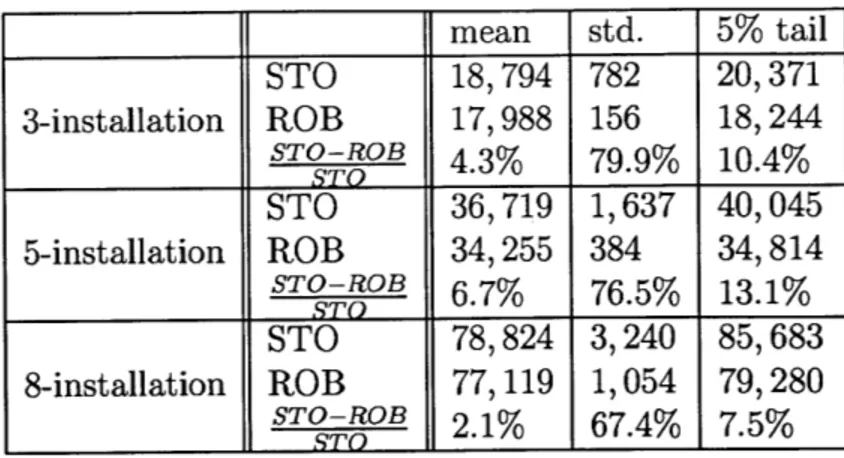
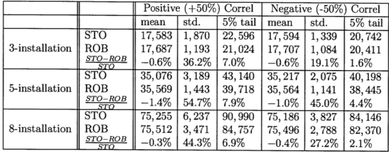
In the second part of the thesis, we propose methods to compute (s,S) policies in supply chain networks using robust and stochastic optimization and compare their performance. Our algorithms handle general uncertainty sets, arbitrary network topologies, and flexible cost func-tions including the presence of fixed costs. The algorithms exhibit empirically practical running times. We contrast the performance of robust and stochastic (s,S) policies in a numerical study, and we find that the robust policy is comparable to the average performance of the stochastic policy, but has a considerably lower standard deviation across a variety of networks and realized demand distributions. Additionally, we identify regimes when the robust policy exhibits partic-ular strengths even in average performance and tail behavior as compared with the stochastic policy.

Thesis Supervisor: Dimitris Bertsimas

Title: Boeing Professor of Operations Research Co-Director, Operations Research Center

Thesis Supervisor: David Gamarnik

Acknowledgments

I would like to take a moment to mention and thank the people who have played an important

role in my life over the last five years. This section alone can easily be the length of a Chapter. The amount of people who have played a positive role in my life over the last five years, along with their specific acts of kindness, are too many to recount. I have tried my best to name all of the people I can think of, but I apologize ahead of time to those I may have overlooked.

Firstly, I would like to thank my advisers - _{Dimitris Bertsimas and David Gamarnik. As a}

result of your guidance and support, I was able to grow and develop as a researcher and as a communicator. You helped me learn how to frame complex problems and think in big picture terms, and your committment to high quality is a true role model. Most importantly, I was able to grow not just on a professional, but on a personal level as well.

I never would have come to the ORC, if it were not for Chris Wiggins, Patrick Gallagher,

and Ioannis Karatzas. Thank you for providing me with valuable advice, inspiration, and encouragement to pursue a Ph.D. Thank you Kostas Kardaras for your help and advice about graduate school. And thank you Burton Levine for your support and advice.

I would like to specially thank Gabriel Bitran and Eleni Pratsini for providing me with wonderful support, mentorship, and encouragement over the last few years. I am very fortunate that I was able to get to know you. I would like to thank Rama Ramakrishnan, Don Rosenfield, and Leonid Kogan for their valuable advice and encouragement.

90 % of this work was done in the Dewey Library, and I would like to thank the staff of

Dewey for providing such a nice environment for thinking and working. A very special thank you to the staff of the ORC - _{Andrew, Laura, and Paulette. You provided me with wonderful}

help and advice in important times. I would also like to thank Patrick Jaillet for being a great co-director of the ORC.

Thank you to my colleagues and friends at the ORC including Matt Fontana, Maxime, Phil, Joline, Andre, Jason, Adam, Chaithanya, Nick, Shubham, Gareth, Shashi, Xin, Diana, Matthieu, Andy, Eric, Theo and all other pals in the ORC. Thank you to ORC alums Ilan Lobel, Margret Bjarnadottir, Doug Fearing, Dan Iancu, Karima Nigmatulina, Rajiv Menjoge, and Lavanya Marla for your friendship and advice in important times.

In addition to doing research and classwork, I was able to find some free time for other activies such as tennis and coffee. As a result, I have shared wonderful and engaging moments with Ruben Lobel, Nikos Trichakis, Jon Kluberg, Dave Goldberg, Adrian Becker, and Martin

Quinteros.

Thank you for your friendship. Working on projects with Nikos was awesome. Special thanks to Ruben, Nikos, and Martin for introducing me (multiple times) to fine South American meat specialties. A special thanks to Jon for his support over the years and for introducing me to Harvard Chabad. On the tennis front, a very special thanks to Julianne Dunkel, Charlie Maher, and Florin Ciocan for being great tennis partners and great pals. A special thanks to Dima Katz for his personal friendship and collaboration on work in Chapter

3. I learned a great deal from you.

My non-ORC friends including Andres Abin-Fuentes, Gene, Pasha Lavitas, Yura Tarasula,

Nika Gelfand, Artem Stavisky, Dmytro Karabash, Rob Toth, and Jim Kincade made my last five years fulfilling and fun. Thank you for your friendship and for being part of my life. Thank you to Rabbis Posner, Gluckin, and Wiener for your friendship and guidance.

Thank you to my high school homeys Carl Wivagg, Vlad Turzhitsky, and Alex Gordon. I am truly lucky for your support and friendship. The bike trips, camping trips, math team, and business are great times in my life.

Thank you Dasha. I am really happy and lucky you decided to be a Shliach in Boston in

2009.

I would like to thank my family. Thank you to my aunts Galya and Liuda and my cousin Alena for your support and love. Thank you to my mom Vera, dad Anatoliy, and grandparents Bella, Mitya and David for providing me with encouragement and support in times that matter most. I am lucky and grateful for you.

Contents

1 Introduction

1.1 _{Optimization Under Uncertainty. . . . .}

1.2 Thesis Overview and Contributions . . . .

2 Performance Analysis of Queueing Networks via Robust Optimization

2.1 Introduction . . . . 2.2 M odel description . . . . 2.2.1 A tandem single class (TSC) queueing network. Stochastic model . .

2.2.2 _{A multiclass single server (MCSS) queueing system. Stochastic model}

2.2.3 Robust optimization type queueing systems . . . . 2.2.4 The Law of the Iterated Logarithm . . . .

2.3 M ain results . . . .

2.4 Tandem single class queueing system: proof of Theorem 2.2. . . 2.4.1 General upper bound on the sojourn times . . . . 2.4.2 Proof of Theorem 2.6 . . . .

2.5 Multiclass single server queueing system: proofs of main results

2.5.1 Proof of Theorem 2.4 . . . . 2.5.2 Proof of Corollary 2.5 . . . . 2.6 Conclusion . . . . 15 . 15 . 17 21 21 24 24 26 . . . . 29 . . . . 30 . . . . 32 . . . . 35 . . . . 36 . . . . 38 . . . . 40 . . . . 40 . . . . 44 . . . . 45

3 Robust Optimization Analysis of the GI/GI/m Queue 3.1 Introduction . . . .

3.2 GI/GI/m model description . . . . 3.2.1 Stochastic model . . . .

3.2.2 Robust model . . . .

3.3 M ain results . . . .

3.4 Performance bounds in the Halfin-Whitt Regime . . .

3.5 Proofs of Main Results . . . . 3.5.1 Waiting Time: Proof of Theorem 3.1 . . . . .

3.5.2 Queue Length: Proof of Theorem 3.3...

3.6 Conclusion . . . .

4 (s,S) Policies in Supply Chain Networks: Robust vs.

4.1 Introduction . . . . 4.2 The Model. 4.2.1 4.2.2 4.2.3 4.2.4 4.3 The

Notation and Dynamics of the General Assembly System Robust vs. Stochastic Optimization . . . . Designing Uncertainty Sets . . . . Extensions . . . . Algorithms for Robust and Stochastic (s,S) Policies . . . . . 4.3.1 Robust Algorithm. . . . . 47 . . . . 49 . . . . 49 . . . . 50 . . . . 52 . . . . 54 . . . . 58 . . . . 58 . . . . 60 . . . . 66 Stochastic Optimization 67 . . . . 67 . . . . 70 . . . . 70 . . . . 72 . . . . 73 . . . . 76 . 79 . . . . . 81

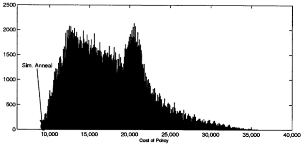
4.3.2 Simulated Annealing and the Robust Algorithm Implementation 4.3.3 Stochastic Algorithm . . . . 4.4 Numerical results . . . . 4.4.1 Effectiveness of Simulated Annealing . . . . 4.4.2 The Networks . . . .

4.4.3 Running Time of the Algorithms . . . . 84 4.4.4 Performance of Robust and Stochastic (s,S) Policies . . . . 85

4.5 Conclusion . . . . 94

5 Concluding Remarks 97

A Technical Results 99

List of Figures

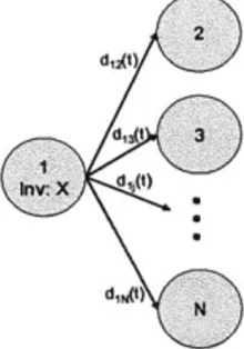
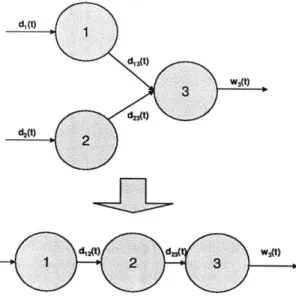
An N installation network. . . . . 3-Installation Setup . . . . Parallel to series transformation.. . . . Comparison of enumeration scheme and Comparison of enumeration scheme and 3-Installation Setup . . . . 5-Installation Setup . . . . 8-Installation Setup . . . . 5-installation: ROB vs. STO - discrete i

50% realized demand correlation . -50% realized demand correlation

SA fc SA fo realiza r the robust r the stocha tion . . . .

4-12 8-installation: ROB vs. STO - Gamma([t, -) realization.

. . . . 74 . . . . 76 . . . . 77 model. . . . . 83 stic model. . . . . 83 . . . . 84 . . . . 85 . . . . 85 . . . . 88 . . . . 90 . . . . 90 . . . . 92

4-13 Relative % performance of ROB vs. STO as a function of realized &. 4-1 4-2 4-3 4-4 4-5 4-6 4-7 4-8 4-9 4-10 4-11

List of Tables

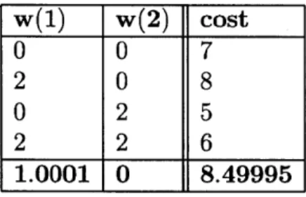
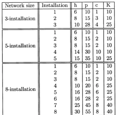
4.1 Costs for various demand realizations . . . . 79

4.2 Cost parameters for the network experiments. . . . . 86

4.3 Run time results (in hours). . . . . 86

4.4 Max cost comparison for polyhedral uncertainty of varying size. . . . . 87

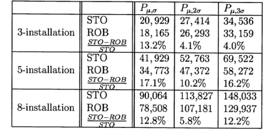
4.5 Comparison of ROB and STO under discrete(p, -) random variable realization. 88 4.6 Comparison of robust and stochastic policies under correlated realized demands. 89 4.7 Comparison of robust and stochastic policies under random continuous demands. 90 4.8 Comparison of robust and stochastic policies under multimodal demands. . . . . 92

4.9 Performance of robust and stochastic policies as a function of realized demand o-. 93 4.10 Key ROB-STO relative performance insights. . . . . 95

Chapter 1

Introduction

The purpose of this thesis is to propose a new method of analysis for queueing systems that leads to explicit upper bounds on performance and to investigate the effectiveness of this method of analysis to the performance of inventory systems. The key approach is to utilize robust optimization, a tractable method to optimize systems under uncertainty that has been widely developed in the last decade. For this reason, we discuss in Section 1.1 optimization under uncertainty and robust optimization, in particular. In Section 1.2, we provide an overview of the thesis and of our contributions.

1.1

Optimization Under Uncertainty

Capturing uncertainty in optimization problems provides a powerful modeling framework. Port-folio optimization, stochastic shortest paths, queueing systems, and revenue management are among the numerous potential problems that can be modeled as optimization problems un-der uncertainty. The downside is that barring very specific examples and models, optimization problems under uncertainty are hard and there are no general and simple tools for solving them. However, throughout the optimization literature there have been several major lines of research to tackle this area, and we outline some below.

One approach known as Stochastic Programming refers to methods that represent uncertain data through scenarios. These scenarios are generated as a result of assuming an underlying

probability distribution for the uncertain parameters. For instance, stochastic linear program-ming finds an optimal solution that produces the best average objective function value over all scenarios. One may then extend this approach to model multi-stage problems using techniques such as Benders decomposition or incorporate a notion of risk into the objective function. The book by Shapiro et al. (Shapiro, Dentcheva, and Ruszczynski 2009) is a standard reference on

stochastic programming.

Dynamic Programming introduced by Richard Bellman is another method designed to deal with uncertain systems. For the most part, dynamic programming also models uncertainty with a probability distribution but is geared towards problems with multiple stages. The spirit of the approach is to solve the problem recursively -starting with the last stage. Often times, the major power of the Dynamic Programming approach is two-fold: it allows the user to prove that a particular policy or solution is optimal, or it allows the user to prove that the optimal policy has a special structure which may greatly reduce the search space for the optimal policy or give rise to good heuristics. We refer the reader to the seminal book by Bellman (Bellman 1957) and the books by Bertsekas (Bertsekas 1995).

Perhaps the greatest drawback of the Stochastic and Dynamic Programming approaches is that they suffer from the curse of dimensionality. In other words, barring specialized mod-els, the solution time of these problems increases exponentially with the size of the problem (e.g. number of stages). Another method for incorporating uncertainty into optimization prob-lems is known as Robust Optimization. For a review of robust optimization see the survey

by Bertsimas et al. (Bertsimas, Brown, and Caramanis 2011) and the book by Ben-Tal et al.

(Ben-Tal, Ghaoui, and Nemirovski 2009). Robust optimization provides a tractable framework for incorporating uncertainty into the optimization problem. Robust Optimization does not model uncertainty with a specific probability distribution, but instead models uncertainty with uncertainty sets (polyhedra or ellipsoids). The main impact of robust optimization is two fold: First, it allows the decision maker to include uncertainty information into the optimiza-tion problem, whereas other methods may fail completely due to tractability issues. Secondly, robust optimization provides a particular advantage for modeling in low data environments (forecast is poor) by avoiding strong assumptions about the underlying probability distribution for uncertain parameters.

theory and application fronts. Researchers are still trying to figure out the extent to which this framework can be applied to model real world problems. Additionally, robust optimiza-tion has a deep underlying connecoptimiza-tion to risk theory (Natarajan, Pachamanova, and Sim 2009; Bertsimas and Brown 2009) and as a result provides a tractable framework for which to model problems that have hitherto been attacked with traditional stochastic approaches. Thus, it is a very exciting and potentially rewarding pursuit to push the envelope of the robust optimization modeling framework to see how well one can model and capture complex random behavior (i.e. in queueing systems or finance) in a tractable manner (i.e. in a linear or quadratic program) that agrees qualitatively with probabilistic methods.

1.2

Thesis Overview and Contributions

This thesis is composed of three self-contained essays illustrating the applications of robust optimization approaches. Chapters 2 and 3 both deal with queueing systems and Chapter 4 with inventory theory. The motivation for the research is two fold:

" To use the robust optimization modeling framework for performance analysis in queueing

systems. In particular, the goal is to compute bounds on performance measures for several types of queueing systems using robust optimization in a way that translates to meaningful bounds and insights for the underlying stochastic system.

" Understand the benefits and drawbacks of the policies and solutions to optimization

prob-lems with uncertainty based on the robust optimization approach as compared with tra-dititional stochastic optimization, particularly in the context of inventory systems. We next give a brief overview of each chapter and its specific contributions below:

Chapter 2 considers the question of performance analysis of queueing systems. In this chapter, we propose a new performance analysis method, which is based on robust optimization. The basic premise of our approach is as follows: rather than assuming that the stochastic primitives of a queueing model satisfy certain probability laws, such as, for example, i.i.d. interarrival and service times distributions, we assume that the underlying primitives are deterministic and sat-isfy the implications of such probability laws. These implications take the form of simple linear

constraints, namely, those motivated by the Law of the Iterated Logarithm (LIL). Using this approach we are able to obtain performance bounds on some key performance measures. Fur-thermore, these performance bounds imply similar bounds in the underlying stochastic queueing models.

We demonstrate our approach on two types of queueing systems: Tandem Single Class (TSC) queueing network and the Multiclass Single Server queueing network. In both cases, using the proposed robust optimization approach, we are able to obtain explicit upper bounds on some steady-state performance measures. For example, for the case of TSC system we obtain a bound of the form

C(1 - p)- In ln((1 - p)-')

on the expected steady-state sojourn time, where C is an explicit constant and p is the bot-tleneck traffic intensity. This qualitatively agrees with the correct heavy traffic scaling of this performance measure up to the ln ln((1 - p)-1) correction factor.

Chapter 3 considers the performance analysis of the single class m-parallel server network (GI/GI/m) with general, but independent interarrival and service times. In particular, we

apply the approach developed in Chapter 2 to address the question of computing waiting times and queueing lengths for the GI/GI/m queueing system. Using this approach we are able to obtain explicit bounds on waiting times and queueing lengths of the form

C(1 - p)-' In ln((1 - p)-')

that qualitatively agree with Kingman's bounds up to the the ln ln((1 - p)-4) correction factor.

Additionally, we analyze the waiting time of the GI/GI/m robust model in the Halfin-Whitt regime and compare to how it performs to traditional stochastic analysis. In particular, we explicitly construct and prove an upper and lower bound on the waiting time of the steady state customer in the robust GI/GI/m system. These results indicate that as more servers are added to the system, the steady state customer in the robust GI/GI/m system experiences a decline (upper bound result) in the expected waiting time that is similar to the steady state customer in the stochastic GI/GI/m system. However, as more and more servers are added to the system, the stochastic steady state waiting time is driven to zero, while the robust steady

state waiting time remains strictly above zero.

Chapter 4 addresses the question of computing (s,S) policies in supply chain networks. In

particular, we propose methods to compute (s,S) policies in supply chain networks using robust and stochastic optimization and compare their performance. Our algorithms handle general un-certainty sets, arbitrary network topologies, and flexible cost functions including the presence of fixed costs. The algorithms exhibit empirically practical running times. In a numerical study, we contrast the performance of robust and stochastic (s,S) policies, and we find that the robust policy is comparable to the average performance of the stochastic policy, but has a consider-ably lower standard deviation across a variety of networks and realized demand distributions. Additionally, we identify regimes when the robust policy exhibits particular strengths even in average performance and tail behavior as compared with the stochastic policy.

Chapter 2

Performance Analysis of Queueing

Networks via Robust Optimization

2.1

Introduction

Performance analysis of queueing networks is one of the most challenging areas of queueing theory. The difficulty stems from the presence of network feedback, which introduces a complicated multidimensional structure into the stochastic processes underlying the key performance measures. Short of specialized cases, such as product form networks, which typically rely on Poisson arrival/exponential service time distributional assumptions, the problem is largely unresolved. Specifically, given the topological description of a queueing network and given the description of the underlying stochastic primitives such as interar-rival and service times distributions, we do not have good tools for computing exactly or obtaining upper and lower bounds on key performance measures, such as, for example average queue lengths and waiting times. Some of results which provide non-asymptotic bounds on performance measures can be found in (Bertsimas, Paschalidis, and Tsitsiklis 1994), (Kumar and Kumar 1994), (Kumar and Morrison 2004), (Jin, Ou, and Kumar 1997), (Bertsimas, Gamarnik, and Tsitsiklis 1996), (Bertsimas and Nino-Mora 1999), all of which require Markovian (Poisson arrival/exponential service time) distributional assumptions. Moreover, some of these bounds become quite weak as traffic intensity (of some of the network

components) approach unity. For example, a bound of the form O((1 - p*) 2) is obtained in (Bertsimas, Gamarnik, and Tsitsiklis 2001), where p* is the bottleneck (real or virtual, see the reference) traffic intensity. The other references can lead to infinite upper bounds even in the cases where stationary distribution exists. The approaches in these papers also do not extend to the case of non-Markovian systems. As a consequence, most of the known performance analysis results are of an asymptotic nature, which apply to queueing networks in various limiting regimes, such as the heavy traffic regime (Harrison 1990),(Whitt 2002),(Chen and Yao 2001), large deviations methods (Ganesh, O'Connell, and Wischik 2004),(Shwartz and Weiss 1995), approximations by phase-type distributions (Kleinrock 1975),(Latouche and Ramaswami 1987). In this thesis, we partially fill this gap by developing a new performance analysis approach based on robust optimization methods. The theory of robust optimizaiton emerged recently as a very successful and constructive approach for the analysis of certain stochastic model-ing problems (Soyster 1973),(Ben-Tal and Nemirovski 1998), (Ben-Tal and Nemirovski 1999), (Bertsimas and Sim 2004). The main premise of our approach in the queueing context is that, rather than assuming probabilistic laws for the underlying stochastic primitives, such as, for example, i.i.d. interarrival and service times, we consider a deterministic queueing model and we will assume only the implications of these laws. Specifically we consider implications of the Law of the Iterated Logarithm (LIL). The objective is to find laws which on the one hand hold in the underlying stochastic queueing model and, on the other hand, lead to linear constraints in the formulation of the robust optimization problem, and LIL accomplishes this. We illustrate our approach using two queueing models, namely the Tandem Single Class (TSC) queueing system operating under the First-In-First-Out (FIFO) scheduling policy, and the Multiclass Single Server (MCSS) queueing system operating under an arbitrary work-conserving policy. Motivated by the LIL, we consider constraints of the form E1<i<k Ui < A-'k + IVk InIn k,

for all k > 1. Here (Uk, k > 1) is any of the stochastic primitives of the underlying queueing system, such as, for example, the sequence of interarrival times and A stands for the rate of this stochastic primitive. Using these bounds, we derive explicit bounds on some performance measures such as sojourn time in the TSC system, namely, the time it takes for a job to be processed by all the servers, and the virtual workload (virtual waiting time) in the MCSS sys-tem, namely, the time required to clear the current backlog in the absence of future arrivals. In both models we derive upper bounds on the aforementioned performance measures for the

corresponding deterministic counterpart models and prove that similar bounds also hold for the same performance measures in the underlying stochastic models. In both cases the bounds are of the order 0(1'- In ln 1'p), where p is the (bottleneck for the case of TSC model) traffic inten-sity. This matches the correct 0(9.-) order short of ln In((1 - p)- 1_{) error. While the technical}

derivation of these bounds is involved, the conceptual approach is very simple. An interesting distinction of our approach from other robust optimization type results is that our results are explicit, as opposed to numeric results one typically obtains from the formulating and solving a robust optimization model. These explicit bounds however, come at a price of not caring much for the constants corresponding to the leading coefficient. In order to keep things simple we sometimes use very crude estimates for such constants.

Our approach bears similarity with some earlier works in the queueing literature. Specifi-cally, the pioneering work of Cruz (Cruz 1991a), (Cruz 1991b) used a similar non-probabilistic approach to performance analysis by deriving bounds based on placing deterministic constraints on the flow of traffic called "burstiness constraints". The method could be applied to fairly gen-eral network topologies and led to more research in the area. In (Gallager and Parekh 1993), (Gallager and Parekh 1994), tighter performance bounds were obtained assuming a "Leaky Bucket" rate admission control from (Turner 1986) and particular service disciplines. In addi-tion, there is some similarity between the philosophy of our approach and the adversarial

queue-ing network approach (Andrews, Awerbuch, Fernandez, Kleinberg, Leighton, and Liu 1996),

(Borodin, Kleinberg, Raghavan, Sudan, and Williamson 2001), (Goel 1999), (Gamarnik 2003), (Gamarnik 2000), which emerged in the last decade in the computer science literature and also replaces the stochastic assumptions with adversarial deterministic ones. The deterministic con-straints used in the aforementioned works are of the form of A(t) At

+

B where A(t) is the

number of external arrivals into the queueing system up to time t and A represents the ar-rival rate. As it turns out, these types of assumptions are too restrictive from the probabilistic point of view and do not lead to bounds on the underlying stochastic network: observe that every renewal process A(t) arising from an i.i.d. sequence with positive variance violates this assumption almost surely for every B for large enough t. As we demonstrate in this chapter, the constraints motivated by the LIL, namely A(t) At + BVt

InIn

t, can indeed be served to

obtain performance bounds, which can be translated into the underlying stochastic network. In fact, the key contribution of our approach is that the deterministic constraints we place on the

service and arrival processes are rich enough to lead to stochastic results. The results based on "Leaky Buckets", bounded burstiness and adversarial queueing theory address very general queueing networks. It would be an interesting research project to extend our results based on robust optimization to these general network structures.

The rest of the chapter is structured as follows. In the following section we describe two queueing models under the consideration, namely the tandem single class queueing network and the single server multiclass queueing network, as well as their robust optimization counterpart models. Our main results, namely the performance bounds in robust optimization type queueing systems and their implications for stochastic queueing systems are stated in Section 3.3. The proofs of our main results are in Sections 2.4 and 2.5. Some concluding thoughts and directions

for further research are outlined in Section 2.6. Several technical results necessary for proofs of main theorems are delayed untill the Appendix section.

We close this section with some notational conventions. In stands for the logarithm with natural base. The notation (x) I for a non-negative vector x E Rd means applying the square root operator coordinate-wise: (x)i = (x,1 < i < d). AT denotes a transposition operator applied to the matrix A.

2.2

Model description

We now describe the two queueing models analyzed in this chapter, both very well studied models in the literature. We begin by describing these models in the stochastic setting, and then we describe their deterministic robust optimization counterparts.

2.2.1

A tandem single class (TSC) queueing network. Stochastic

model

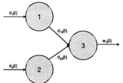
The model is a tandem of single servers S1,..., Sj processing a single stream of jobs arriving from outside and requiring services at S1, ... , S in this order. The jobs arrive from outside according to an i.i.d. renewal process. Let U1, U2, U3,... denote i.i.d. interarrival times with a

arrives. The external arrival rate is defined to be A A 1/E[U1] and the variance of U1 is denoted

by o-2.

The jobs arriving externally join the buffer corresponding to server S1 where they are served using First-In-First-Out (FIFO) scheduling policy. We assume that all buffers are of infinite capacity. After service completion, jobs are routed to the buffer of server S2, where they are also served using FIFO scheduling policy, then they are routed to servers S3, S4, etc. After

service completion in server Sj the jobs depart from the network. Let V denote the service time requirement for job k in server

j.

We assume that the sequence (V, k > 1) is i.i.d. for each

j,

and is independent from all other random variables in the network. The distribution of the service time in server

j

is F,,(t) = P(V' t), t > 0. The service rate in server S is defined

to be pg A _{1/E[Vf], and we denote by pmin = miniy<jp pj the rate of the slowest server. 02} denotes the variance of V/7 for each j = 1,... , J. The traffic intensity in server Sj is defined to

be p3 = A/pyg, and the bottleneck traffic intensity is defined to be p* = maxj pj = A/pmin.

Denote by Wjk the waiting time experienced by job k in server j not including the service time Vkj. Let Wk =

EZ(Wk+V)

be the sojourn time of the job k. Namely, this is time between

the arrival of job k into buffer 1 and service completion of the same job in buffer J. Denote by

Qj(t) the queue length in server

j

(the number of jobs in buffer

j)

at time t. We assume that initially all queues are empty: Qj(0) = 0, 1 <

j

5 J, although most of our results can either be

easily adopted to the case of non-zero queues at time zero, or apply to the steady-state measures where the initializations of the queues is irrelevant. Let Ik denote the idle time of server

j

in between servicing jobs k - 1 and k for k = 2,..., N. We define I = 0 Vj =1,...,J.

The model just described will be denoted by TSC(St) (Tandem Single Class Stochastic) for short. It is known (Sigman 1990),(Dai 1995),(Dai and Meyn 1995),(Chen and Yao 2001) that as long as p* < 1, and some additional mild conditions hold, such as finiteness of moments, TSC(St) is stable and the stochastic processes underlying the performance measures such as queue lengths, workloads, sojourn times are mixing. Namely, these processes are positive Harris recurrent (Dai 1995),(Meyn and Tweedie 1993), and the transient performance measures con-verge to the (unique) steady-state performance measures both in distributions and in moments. Computing these performance measures is a different matter, however. We denote by Wj, Woo the steady state versions of the random variables W,3, Wk. Thus provided that p* < 1 and some

additional technical assumptions hold, we have

lim E[Wn] = E[Woo]. (2.1)

n-+oo

We will assume that p* < 1 holds without explicitly stating it. Rather than describing the assumptions required to make (3.1) true, we will simply assume when stating our results that

(3.1) holds as well.

2.2.2

A multiclass single server (MCSS) queueing system.

Stochas-tic model

We now describe our second queueing model. Consider a single server queueing system which processes J classes of jobs. The jobs of class

j

= 1, 2,..., J arrive from outside according to

a renewal process with i.i.d. interarrival times U', k > 1 and distribution function Fa,j (t)

P(Uf < t). The arrival rate for class

j

jobs is Aj A 1/E[Ufl]. It is possible that some classes

j

do not have an external arrival process, in which caseUk = o almost surely and Aj = 0. Let

o., be the variance of Uj. The sequences (Uk, k > 1) are also assumed to be independent for

different

j.

Let A = (A3) denote the J-vector of arrival rates. We let Amax = maxi<,<j Aj and Amin = mini<<j Aj. We let A(t) = (Aj(t)) denote the vector of cumulative number of external

arrivals up to time t where Aj (t) = max{k: E1<i<k Uj < t}

The jobs corresponding to class

j

are stored in buffer By until served. As in the single class case, we assume all buffers are of infinite capacity. The service time for the k-th job arriving to buffer Bj is denoted by Vj and the sequence (Vkj, k > 1) is assumed to be i.i.d. with a common distribution function F,,j(t) = P(Vj <; t). Additionally, these sequences are assumed to be independent for all

j

and independent from the interarrival times sequences (Uk, k > 1). The average service time for class

j

is my j E[V'] and the service rate is j A 1/E[Vlf]. o

denotes the variance of V1'. Let fm- = (my) denote the J-vector of average service times and let

p = (py) be the J-vector of service rates. Let M denote the diagonal matrix with j-th entry

equal to paj and let pma = maxi<ji ij.

We assume that the jobs in buffer By are served using FIFO rule, but prioritizing jobs between different buffers By is done using some scheduling policy 9. The only assumption we

make about 0 is that it is a work-conserving policy. Namely, the server is working full time as long as there is at least one job in one of the buffers Bj, 1

< j <

J. The only performance

measure we will consider is the workload (defined below) for which it is well known that the details of the scheduling policy are unimportant for us, as long as the policy is work-conserving.

The routing of jobs after service completions is determined using a routing matrix P, which is an J by J 0, 1 matrix P = (P, ,1 < i, j < J). It is assumed that

Ej

Pi

<

1 for each i.

(Namely, the sum is either 1 or 0). Upon service completion in buffer Bi, the job of class i is routed to buffer

j

if Pj = 1. Otherwise, if Ej Pj = 0, the jobs of class i leave the network.

It is assumed that P" = 0 for some positive integer n. It is easy to see that this condition is

equivalent to saying that all jobs eventually leave the network.

It is known (Chen and Yao 2001) that the traffic equation Ai = Ai +

EZ

₁ AiPji has a

unique solution A (A3) given simply as A = [I - PT]-1 A, where I is the J by J identity

matrix. Let Ama = maxj(As) (observe that A₃

<

A, for every

j

and hence Amax > Amax). Let

A(t) = (Aj(t)) denote the vector of number of arrivals by time t that will eventually route to

server

j:

Aj

(t) =

e

(I + (pT)1 + (pT)2 +.. .)A(t) = ef[I - PT]-A(t) and ej denotes the j - th

unit vector.

The traffic intensity vector is defined to be p = M-1 = M-1[I - PT]-1A. The traffic intensity of the entire server is p = eTp, where e is the J vector of ones. Let Qj(t) denote the

queue length in buffer

j

at time t, let Q(t) = (Qj(t)). We assume that Q(0) = 1. As for the case

of TSC model, our results can be extended to the case Q(0) > 0, but for the results regarding steady-state behavior, the initialization of queues is irrelevant. Denote by Wk the waiting time of the k-th job arriving into buffer

j.

We let Wt denote the workload at time t. Namely, Wt is the time required to process all the jobs present in the system at time t, in the absence of the future arrivals. Note that Wt is also the virtual waiting time at time t when the scheduling policy is FIFO. Observe that if to marks the beginning of a busy period and ti belongs to the same busy period (namely, the server was working continuously during the time interval [to, ti]), then almost surely

A1(ti) Aj(ti)

Wi = Vl+ ... +

(

V| - (t1 -to). (2.2)

The model described above is denoted by MCSS(St) (Multiclass Single Server Stochastic) for short. It is known (Dai 1995) that if p < 1, and some additional technical assumption on

interarrival and service time distributions hold then MCSS(St) is stable and enters the steady state in the same sense as described for the tandem queueing network. While in this case the steady-state distribution of many performance measures usually depends on the details of work-conserving policy used, the steady-state distribution of the workload does not depend on the policy, as we have discussed above. Let W, denote the workload in steady state, and let B, and I. denote the steady-state duration of the busy and idle periods, respectively. Additionally, denote by Io, B1, I1, B2, I2,... the alternating sequence of the lengths of the busy

and idle periods of the MCSS(St) system, assuming that time zero initiates a busy period. Under the same technical assumptions as above the following ergodic properties hold almost surely:

lim = E[Wo], (2.3)

t-+0o t

lim Bi = E[Bo], (2.4)

n-+oo n

lim <i<n = E[I] (25)

n-+o n

lim l<iyn = E[B2]. (2.6)

n-+o _n

We denote by n(t) the number of busy periods that have been initiated up to time t. Math-ematically, we define n(t) to satisfy Zl<i n(t)-1(Bi + Ii) < t < Zl<i~n(t)(B + Ii). When t E [Z_1i~n(t)l(Bi + Ii), ZEl g y_(t)1l(Bi+I) +Bn(t)], t falls on a busy period and using the def-inition of n(t), we have W(t) < Bn(t). When t C 1<i n(t)-_Z1(Bi+Ii)+Bn(t), Zl<i n(t)(Bi+I)],

t falls on idle period In(t) and hence W(t) = 0. We let r denote the beginning of the i-th busy

period. This implies

f0

W(s)ds _zE2 frinr+Bijt) W(s)ds Ziin(t) Bi

If (2.3),(2.4),(2.5) and (2.6) hold, then we also obtain

E[B] E[B ]

E[WOO] < W] < . (2.7)

-E[Bo] + E[Iw] - E[B W]

This bound will turn useful when we apply our results for robust optimization models to the underlying stochastic model. As for the TSC case, we assume from now on p < 1. Rather than

listing the assumptions leading to ergodic properties (2.3),(2.4),(2.5) and (2.6) we assume when stating our results, that the stochastic process Wt enters the steady-state as t -+ oo and that the properties (2.3),(2.4),(2.5) and (2.6) holds almost surely.

2.2.3

Robust optimization type queueing systems

We now describe deterministic robust optimization type counterparts of the two stochastic queueing models described in the previous subsections.

We begin with TSC model and describe the corresponding model which we denote by TSC(RO) (Tandem Single Class Robust Optimization). The description of the network topol-ogy is the same as for TSC(St). However, it is not assumed that U, Vj and, as a result

Q

(t), Wki, Wk are random variables. Rather we assume that these quantities are arbitrary

sub-ject to certain linear constraints detailed below. Additionally, we assume that the system starts empty Q(O) = 0 and only n jobs go through the system.

Specifically, consider a sequence of non-negative deterministic interarrival and service times

(Uk,1 < k <n),(Vkj,1 <k<n),1<j<J. Let

0(z) = - (2.8)

1, x

<

ee.

We assume that there exist A, I, and paj, F,,j > 0, 1 <

j

< J such that

SUk- A-1(n - k) Fa(n - k), k = 0, 1,... ,n - 1, (2.9)

k+1 i<n

V - -i (n - k)| F,#(n - k), k = 0, 1,...,n - 1,

j

= 1, 2, ... , J. (2.10)

It is because we need to consider tail summation _k+1<i<n we assume that only n jobs going through the system, though we will be able to apply our results in the stochastic setting where infinite number of jobs pass through the system. Let F = max(Fa, r,,). Borrowing from the robust optimization literature terminology (Bertsimas and Sim 2004), the parameters F, F,,, r are called budgets of uncertainty. Note, that the values Uk, V, k > 1 uniquely define the

corresponding performance measures Qj(t), Wi, Wk, k = 1,... , n. There is no notion of steady

state quantities Qj(oo), Woo for the model TSC(RO). The motivation for constraints (2.9) and (2.10) comes from the Law of the Iterated Logarithm, and we discuss the connection in a separate subsection.

We denote the robust optimization counterpart of the MCSS(St) model by MCSS(RO). In this case it turns out to be convenient to consider infinite sequence of jobs. Thus consider infinite sequences of deterministic non-negative values (Uj, k > 1), (Vj, k > 1), 1

<

j

5 J. It is

assumed that values A., jj, Fa,j, ,,j 0, 1

j

J exist such that

IE Uk - Afi k| < r,J#(k, k = 1, 2, ...,7 j = 1, 2,. .. J, (2.11)

1<i<k

V -

tip

1

_k|

_{Fs,,o(k), k = 1, 2, ... , j = 1,2,..., J. (2.12)}

l<i<k

For convenience we assume that at time zero the system begins with exactly one job in every class

j

= 1, ... , J: Qj(0) = 1. Then the first after time zero external arrival into buffer j occurs

at time Uji. As before, we let F = max(Fa,j, L.,i).

For technical reasons, we also assume that F in TSC(RO), MCSS(RO) constraints satisfies AF > e2e and min Ar > e2e, respectively. (2.13)

3

2.2.4

The Law of the Iterated Logarithm

One of the cornerstones of the probability theory is the Law of the Iterated Logarithm (LIL) (Chung 2001), which states that given a i.i.d. sequence of random variables X1, ... , X, ... with

zero mean and finite variance o-, the following holds almost surely,

lim sup - 1, lim inf X -1.

n->oo oV2nlnlnn n-+oo o-v2nln ln n

The LIL extends immediately to non-zero mean i.i.d. sequences by subtracting nE[Xi] from E <k<n Xk. Furthermore, LIL implies (in the case of zero-mean variables) that

]LIL A sup | X < 00, (2.14)

n>1 o-24(n)

where

4

is defined in (3.2). Note that 1 1_{UL is a random variable. Thus when we consider}

stochas-tic queueing models such as TSC(St) or MCSS(St), the constraints (2.9),(2.10),(2.11),(2.12) hold with probability one, with F = V2FLILo-, where FLIL is defined in (2.14) for the cor-responding random sequence. Specifically, let Va = Fa,LIL = LIL and u = o-a, when

Xk = Un-k - A-1, 0 < k < n - 1 and Uk is the sequence of interarrival times in the TSC(St) model. Similarly define ,J = Fs,J,LIL when Xk = Vk - gi,0 < k < n - 1,1 <

j

5 J.

Observe, that for F, Fs,j thus defined, the constraints (2.9),(2.10) hold for an infinite sequences of jobs (that is jobs which would have indices -1, -2,...), even though we need it only for the first n jobs. For the MCSS(St) model define Fj = ?a,j,LIL, Fs,j = Fs,j,LIL corresponding to the

sequences U - A' , Vj - A3l, k > 1, respectively. We obtain

Proposition 2.1 Constraints (2.9),(2.10),(2.11),(2.12) hold with probability one for Fa -v(Fa,LILa, FS,j = VFs,j,LILUs,j, Fa,j = VFa,j,LILUa,j, and F,j = v2Fsj,LILTsj, respectively,

where F.,.,LIL is defined in (2.14) for the corresponding sequence.

As a conclusion, for every property derivable on the basis of these constraints in our de-terministic robust optimization queueing network models, such as, for example, bounds on the sojourn time of the n-th job in TSC, the same property applies with probability one for the underlying stochastic network. This observation underlies the main idea of the work.

2.3

Main results

In this section we state our main results on the performance bounds for robust optimization type queueing networks TSC(RO) and MCSS(RO), and the implications of our results for their stochastic counterparts TSC(St) and MCSS(St). We begin with TSC(RO) with the goal of obtaining a bound on the sojourn time.

Theorem 2.2 The sojourn time of the n-th job in the TSC(RO) queueing system with con-straints (2.9),(2.10) satisfies

Wn < In

In

+ JA-1. (2.15) 1-

ip* _p*

Observe that the bound on the sojourn time is explicit. It is expressed directly in terms of the primitives of the queueing system such as arrival and service rates. Observe also that the upper bound is independent from n. One can think of this bound as a "steady-state" bound on the sojourn time in the robust optimization model of the TSC system. Additionally, the constant F2

is related to the "variances" of interarrival and service times viz a vi the LIL (2.14). It is known that in the stochastic GI/GI/1 queueing system the expected waiting time in steady state is approximately (oU +o2)/(2A(1 -p)), when the system is in heavy traffic, namely p -+ 1. Namely, the expected waiting time depends linearly on the variances of interarrival and service time. Our bound (2.15) is thus consistent with this type of dependence. On the other hand, unfortunately, our bound depends quadratically on the number of servers J, whereas the correct dependence is known to be linear, at least in some special cases (Reiman 1984),(Gamarnik and Zeevi 2006). The bound above does not have a correct O((1 - p*)-) scaling, which is known to be correct

from the heavy-traffic theory perspective (Reiman 1984),(Gamarnik and Zeevi 2006). However, the correction factor is a very slowly growing function In ln. The upshot is that we can use this bound to obtain a bound on W,-, and Wo. in the underlying stochastic system. This is what we do next.

network satisfies

E[Wn] 5 E 7_{jFA in In I j + JA . (2.16)}

11 - p* 1 - p*1

where F = max,(vuo-aFa,LIL, V2o-s,jFsj,LL, e2eA-1). If in addition the assumption (3.1) holds then

E[Woo] < E7j2A In In + JA- 1. (2.17)

11 - p* 1 - p*1

Proof. We first assume Theorem 2.2 is established. Note, in the context of the stochas-tic system, both Wn and F in Theorem 2.2 are random variables. We take F =

max(v/o-ara,LIL, ov-s,jrs,j,LIL, e2e /-) to satisfy (3.6), where F.,.,LIL is defined in (2.14) for

the corresponding sequence. Applying Proposition 2.1 we have that (2.15) holds with proba-bility one for the underlying stochastic network. The bound (2.16) now follows from taking expectations of both sides of (2.15). The bound (2.17) follows from applying (3.1) to (2.16). 0

We now turn our attention to the MCSS queueing model. Our approach for deriving a bound on the workload is based on first obtaining an upper bound on the duration of the busy period. Thus, we first give a bound on the duration of the busy period and then turn to the workload. Recall our assumption Q(O) = 1, though our results can readily be extended to the general case

of Q(O) > 0. Thus, time t = 0 marks the beginning of a busy period.

Theorem 2.4 Given a MCSS(RO) queueing system with constraints (2.11),(2.12), let B be the duration of the busy period initiated at time 0. Then

5(4J + 3)2_A3 _p4 _{2(4J + 3)X2nax} 2

max

mmx

B < _B- (1-p) _(1i-p)2 ln In _{i-_p} , (2.18) 2(4J + 3)23 mxr4 (4J+ 3) 2a p2

and sup W(t) < lnin nnax max + F 31ax p3. (2.19)

O<t<B 1 - P

1

- p

While the bound (2.19) corresponds to the maximum workload during a given busy period, the actual value of the bound does not depend on the busy period length explicitly. As it will

become apparent from the proof, we use the same technique for obtaining a bound simultane-ously on the duration of the busy period and maximum workload during the busy period. Let us now discuss the implications of these bounds for the underlying stochastic model MCSS(St).

Corollary 2.5 Given a MCSS(St) model, suppose the relations (2.3),(2.4),(2.5) and (2.6) hold. Then 5(4J+ 3)2 3 r4 2(4J + 3)A2 r2

E{Bo]

_E (I 2a In ln max' (2.20) (1- p)2 _{1 - p} 25(4J+ 3) 4A'naxmLmaxF8 2(4J+3)X222] E[Wo] <E P), (lnn 2 a (2.21) (1-p)i-p where F = maxj

(2o-/,ca,,

],j,L1L, e2,A- 1

Unfortunately, in this case the scaling of our bounds as p -+ 1 deviates significantly from the correct behavior. From the heavy traffic theory (Dai and Kurtz 1995), the correct behavior for the steady-state workload should be O((1 - p)- 1). As for the steady-state busy period,

the theory of M/G/1 queueing system (Kleinrock 1975) suggests the behavior O((1 - p)-1)

as opposed to O((1 - p)-21n In(1 - p)-) which we obtain. On the positive side, however, we managed to obtain explicit bounds on the performance measures which are expressed directly in terms of the stochastic primitives of the model, which we do not believe was possible using prior methods. We leave it as an interesting open problem to derive the performance bounds based on the robust optimization technique, which lead to the correct scaling behavior as p - 1.

While the proofs of our main results are technically involved, conceptually they are not complicated. Before we turn to formal proofs, in order to help the reader, we outline below informally some of the key proof steps for our results.

For the TSC queueing network we first replace the constraints (2.9),(2.10) with more general constraints, see (2.22) and (2.23) below. Our results for the TSC network rely mostly on the Lindley's type recursion which in a single server queueing system recursively represents in the waiting time of the n-th job in terms of the interarrival and service times of the first n jobs. It is classical result of the queueing theory that this waiting time can be thought of as maximum of a random walk, with steps equalling in distribution to the difference between the interarrival

and service times. We derive a similar relation in the form of a bound on the sojourn time of the n-th job in the TSC network. This bound is given in Theorem 2.6. Then we view this bound as an optimization problem and obtain a bound on the objective value by proving the concavity of the objective function and substituting explicit bounds from constraints (2.9),(2.10).

Our proofs for the MCSS queueing system rely on the relation (2.2). Namely, we take advantage of the fact that the workload is depleted with the unit rate during the busy period. Then we take advantage of the constraints (2.11),(2.12) to show that in the MCSS(RO) system the workload at time t during the busy period can be upper bounded by an expression of the form -at

+

bVt ln lnt

+

c with strictly positive a, b. It is then not hard to obtain an explicit estimated

to such that this expression is negative for t > to. Since this expression is an upper bound on a non-negative quantity (workload), then the duration of the busy period cannot be larger than to. This leads to an upper bound on the duration of the busy period in the MCSS(RO) system. In order to obtain a bound on the workload, we again take advantage of (2.2) and further obtain explicit upper bounds on the terms involving the sums of service times. We show that the workload at time t is at most -at

+

bv/T In-In t

+

c. We then obtain an upper bound on the

workload during the busy period by obtaining explicit bounds on maxt>o -at

+

bvt ln ln t

+

c.

Our derivation of the bounds for the stochastic model MCSS(St) relies on the ergodic rep-resentation (2.3). We consider a modified system in which each busy period is initiated with simultaneous arrival of one job into every buffer

j.

This leads to a alternating renewal process with alternating i.i.d. busy and idle periods. We then obtain a bound on the steady-state workload in terms of the second moment of the busy period in the modified queueing system, using the renewal theory type arguments. It is this necessity to look at the second moment of the busy period which leads to a conservative scaling

o((1

-p)- 4(ln ln(1 _p)-1)2) in our bound

(2.21) on the steady-state workload.

2.4

Tandem single class queueing system: proof of

The-orem 2.2

In order to prove Theorem 2.2 we first generalize constraints (2.9),(2.10) and obtain a method for bounding W, under more general uncertainty assumptions.

2.4.1

General upper bound on the sojourn times

Given a sequence of non-negative real values Vin(k), max (k) 1 _{< j < J, 1 <k< n,}

Fmin(k), J'max(k) 1 < k < n, we consider the set of all sequences of service times and

inter-arrival times (V), (U)

j

= 1,..., J, i = 1, ... ,n satisfying for all k = 1, ... n n mina(k) < E imaxk(k)Vj < i=k Fmin(k) < 1 Ui <; Fmax(k), i=k (2.22) (2.23) V3, U i' ;> 0.

-In the next theorem we obtain a bound on the sojourn time of the n-th job in TSC(RO) system in terms of values Fin(k), iax(k), Fmin(k), Fmax(k).

Theorem 2.6 Suppose the relations (2.22) and (2.23) hold. Then

J-1

W < max >I :l(F- 7ax(k) - Fin(k ₃+₁ + 1)) + Finax(kj)

n>k>...>ki>a1

- Fmin(ki

+

1)

We now show how Theorem 2.6 implies our main result Theorem 2.2.

Proof of Theorem 2.2. The proof consists of two steps: the first step uses Theorem 2.6 to bound

Wn with uncertainty sets (2.9),(2.10). The second step involves solving some associated maxi-mization problem.

We set Fmin(k) = A-1(n + 1 - k) - Fa4(n + 1 - k), Imax(k) = A- 1(n + 1 - k) +

Fa4(n + 1 - k),7jn(k) = p.j(n + 1 - k) -F₈ ,54(n+1-k), a(k) = p'i-(n + 1 - k) +

17,j4(n + 1 - k), where

#

is defined by (3.2). From Theorem 2.6 we obtain: J-1 W,, < max Y (p-1(n + 1 - k) + ,j#(n + 1 - k)) n>kj>...>ki>1 j=1 J-1 - (pit;(n + 1 - kj+1 - 1) - T',s#(n + 1 - kj+1 - 1)) j=1 + (pil(n +1 - k) + sJ#(n +1 - k)) - (A\- 1 (n + 1 - ki - 1) - Fab(n + 1 - ki - 1))

Since n > kj+1 kj Vj, we can replace p.( by p.z-1 = max(-,' ... , p5) < A- and

preserve inequality. Similarly, we can replace F's,1, Fs,2 , -.. , s,J, IFa by F. We obtain:

max

nkj>...>k1>1

+ (pt-1(n + 1 - kg) + F#(n + 1 - ks)) - (A(n - k) - F#(n - ki))

k max (n - kl) + 2J4(n + 1 - ki)

n~ki>1

+ Jy-; - A'(n - ki) where we used k, < k2 < ... < kj to combine F terms

= max (n + 1 - k1)(pL- - A-') + 2Jo(n + 1 - ki) + (J - 1)I + A

n>ki>1

< max (n + 1 - k1)(p- - A') + 2JF#(n + 1 - ki) + JA'

n>ki>1 since A-1 > Lmi

We let x = n + 1 - k1. Since 1 < k, < n we have that 1 < z < n and obtain:

Wn < max x(p- - A-') + 2JF#(x) + JA-1

< max x(p-1 - A-') + 2JF#(x) + JA-1 (2.25)

X>1 a=n

Putting a = A-' - p-1n 7b = JJ',c = J.)J1, and using the assumption (3.6), we have b/a=

AJF/(1 - p*) > e2e, namely, the condition (A.1) is satisfied.

Appendix we obtain

7A J2_F2

W, < ln In

- 1 p*

Applying Proposition A.3 from

AJF 1- + JA~1. 1- p* Wn < J-1 y [/C1(kj+1+1I - kj) + F(#(n + 1 - ky) +

4(n

- kj+1))