Effect of land albedo, CO₂, orography, and oceanic heat transport on extreme climates

HAL Id: hal-00298120

https://hal.archives-ouvertes.fr/hal-00298120

HAL is a multi-disciplinary open access

archive for the deposit and dissemination of sci-entific research documents, whether they are pub-lished or not. The documents may come from teaching and research institutions in France or abroad, or from public or private research centers.

L’archive ouverte pluridisciplinaire HAL, est destinée au dépôt et à la diffusion de documents scientifiques de niveau recherche, publiés ou non, émanant des établissements d’enseignement et de recherche français ou étrangers, des laboratoires publics ou privés.

Effect of land albedo, CO2, orography, and oceanic heat

transport on extreme climates

V. Romanova, G. Lohmann, K. Grosfeld

To cite this version:

V. Romanova, G. Lohmann, K. Grosfeld. Effect of land albedo, CO2, orography, and oceanic heat transport on extreme climates. Climate of the Past Discussions, European Geosciences Union (EGU), 2005, 1 (3), pp.255-285. �hal-00298120�

CPD

Full Screen / Esc

Print Version Interactive Discussion

EGU Climate of the Past Discussions, 1, 255–285, 2005

www.climate-of-the-past.net/cpd/1/255/ SRef-ID: 1814-9359/cpd/2005-1-255 European Geosciences Union

Climate of the Past Discussions

Climate of the Past Discussions is the access reviewed discussion forum of Climate of the Past

E

ffect of land albedo, CO

₂

, orography, and

oceanic heat transport on extreme

climates

V. Romanova1, G. Lohmann2,1, and K. Grosfeld2,1

1

Department of Physics, University of Bremen, Otto-Hahn-Allee, 33040 Bremen, Germany 2

Alfred Wegener Institute for Polar and Marine Research, 27515 Bremerhaven, Germany Received: 11 October 2005 – Accepted: 22 November 2005 – Published: 7 December 2005 Correspondence to: V. Romanova (romanova@uni-bremen.de)

CPD

Full Screen / Esc

Print Version Interactive Discussion

EGU Abstract

Using an atmospheric general circulation model of intermediate complexity coupled to a sea ice-slab ocean model, we perform a number of sensitivity experiments under present-day orbital conditions and geographical distribution to assess the possibility that land albedo, atmospheric CO₂, orography and oceanic heat transport may cause

5

an ice-covered Earth. Changing only one boundary or initial condition, the model pro-duces solutions with at least some ice-free oceans in the low latitudes. Using some combination of these forcing parameters, a full Earth’s glaciation is obtained. We find that the most significant factor leading to an ice-covered Earth is the high land albedo in combination with initial temperatures set equal to the freezing point. Oceanic heat

10

transport and orography play only a minor role for the climate state. Extremely low concentrations of CO₂ also appear to be insufficient to provoke a runaway ice-albedo feedback, but the strong deviations in surface air temperatures in the Northern Hemi-sphere point to the existence of a strong nonlinearity in the system. Finally, we argue that the initial condition determines whether the system can go into a completely ice

15

covered state, indicating multiple equilibria, a feature known from simple energy bal-ance models.

1. Introduction

Investigations of glacial carbonate deposits suggest a sequence of extreme Neopro-terozoic climate events (600–800 million years ago). Paleolatitude indicators and

pale-20

omagnetic data (Hoffman, et al., 1998; Schmidt and Williams, 1995; Sohl et al., 1999; Evans et al., 2000) imply widespread equatorial glaciation at sea level. It was hypoth-esised that the Earth was completely ice covered (Kirschvink, 1992; Hoffman et al., 1998; Kirschvink et al., 2000; Hoffman and Schrag, 2002). Still, the question remains, whether the Earth was completely ice covered (“hard snowball” Earth) or some tropical

25

CPD

Full Screen / Esc

Print Version Interactive Discussion

EGU climate system into the glaciated state and which allowed the escape from it.

The “Snowball” Earth hypothesis provoked the interest of many climate modellers (e.g. Crowley and Baum, 1993; Jenkins and Frakes, 1998; Hyde et al., 2000; Chandler and Sohl, 2000; Crowley et al., 2001; Poulsen et al., 2001; Donnadieu et al., 2002; Bendtsen, 2002; Lewis et al., 2003; Donnadieu et al., 2004; Stone and Yao, 2004) to

5

simulate an ice covered Earth. Using different types of models, from simple Energy Balance Models (EBM) (Budyko, 1969; Sellers, 1969) to coupled ocean atmospheric general circulation models (OAGCM) (e.g. Poulsen et al., 2001), the role of the insola-tion, Earth’s rotation rate and high obliquity (Longdoz and Francois, 1997; Jenkins and Frakes, 1998; Jenkins, 2000; Donnadieu et al., 2002) has been investigated.

Further-10

more, the influence of various paleogeography and continental geometries (Poulsen et al., 2002; Donnadieu et al., 2004) during Neoproterozoic era has been analysed. Such extreme climates in the Earth’s history provide the motivation to investigate under what conditions the climate system is susceptible to extreme changes.

Fraedrich et al. (1999) and Kleidon et al. (2000) used a general circulation model

15

to investigate the land albedo effect of homogeneous vegetation extremes – global desert and global forest. It was found that the dominant signal is related to changes in the hydrological cycle and that the altered water and heat balance at the surface has a potential impact on regional climate. Kubatzki and Claussen (1998) and Wyputta and McAvaney (2001) showed that during the Last Glacial Maximum (LGM) the land

20

albedo increased by 4% due to vegetation changes. In addition to this, the influence of the mountain chains and highly elevated glaciers with strong ice albedo feedback leads to large climate anomalies and an alteration of the atmospheric circulation and precipitation patterns (Lorenz et al., 1996; Lohmann and Lorenz, 2000; Romanova et al., 2005). The increase of the oceanic heat transport is also considered to be a crucial

25

factor to prevent Earth’s glaciation. For example, Poulsen et al. (2001) investigated the role of the oceanic heat transport in “snowball” Earth simulations and concluded that it could stop the southward advance of glaciers, such that a “snowball” Earth could not occur. Multiple stable equilibria are found in an aqua-planet simulation performed

CPD

Full Screen / Esc

Print Version Interactive Discussion

EGU with a coupled atmospheric general circulation model with respect to change of the

oceanic heat transport and initial conditions (Lange and Alexeev, 2004): one warm and ice free planet and one cold and icy climatic state. Furthermore, the atmospheric CO₂ level could also lead to a climate instability and a runaway sea-ice albedo mechanism (Poulsen, 2003). The magnitude of the atmospheric greenhouse gas concentrations,

5

causing glaciation, is still under intense debate (e.g. Chandler and Sohl, 2000; Don-nadieu et al., 2004).

In this study, we are interested in the sensitivity of the climate to changes of the land albedo, orography, oceanic heat transport and CO₂ concentration. Using an AGCM of intermediate complexity we investigate the climate response to some extreme

configu-10

rations of the boundary conditions. Therefore, we perform numerical experiments with different land albedo values and analyse scenarios, in which the land is completely cov-ered with oak forests or glaciers. We have chosen sensitivity experiments with extreme orographical and oceanic heat transport forcings, and with respect to the snowball Earth hypothesis, we vary the CO₂ concentrations to some extreme values. We left

15

the land-sea geometry to present or to Last Glacial Maximum distributions. Most of the external parameters which are different of extreme climate states in the earth history (snowball Earth) are held fixed in order to isolate the effect of land albedo, CO₂, and oceanic heat transport with fixed parameters. Our approach is therefore intended as a sensitivity study.

20

The paper is organized as follows: in Sect. 2 the model is briefly described and in the Sect. 3 the results are given. In Sect. 4 the results are discussed and final conclusions are given in Sect. 5.

CPD

Full Screen / Esc

Print Version Interactive Discussion

EGU

2. Methodology

2.1. Model design

The atmospheric general circulation model (AGCM) used in our study is PUMA (Portable University Model of the Atmosphere) developed in Hamburg (Fraedrich, 1998; Lunkeit et al., 1998). It is based on the primitive equations transformed into

dimension-5

less equations of the vertical component of absolute vorticity, the horizontal divergence, the temperature, the logarithm of the surface pressure and the specific humidity. The equations are solved using the spectral transform method (Orszag, 1970; Eliasen et al., 1970), in which the variables are represented by truncated series of spherical har-monics with wave number 21. The calculations are evaluated on a longitude/latitude

10

grid of 64 by 32 points, which corresponds approximately to a 5.6◦ resolution in Gaus-sian grid. In the vertical direction five equally spaced, terrain-following sigma levels are used. The land and soil temperatures, soil hydrology and river runoff are parameterized in the model.

PUMA is classified as a model of intermediate complexity (Claussen et al., 2002) and

15

it is designed to be comparable with comprehensive AGCMs like ECHAM (Roeckner et al., 1992). Previously, it was used to study stormtracks and baroclinic life cycles (e.g. Frisius et al., 1998; Franzke et al., 2000) and to investigate multidecadal atmospheric response to the North Atlantic sea surface temperatures (SST) forcing (Grosfeld et al., 20051as well as to simulate glacial climates (Romanova et al. 2005).

20

PUMA is coupled to a mixed layer ocean model, which allows the prognosis of the sea surface temperatures (SST). The mixed layer ocean is forced with the oceanic heat transport and its depth is fixed at 50 m. A simple zero layer thermodynamic sea ice model is also included. The temperature gradient in the sea ice is linear and

elimi-1

Grosfeld, K., Lohmann, G., Rimbu, N., Lunkeit, F., and Fraedrich, K.: Signature of atmo-spheric multidecadal variations in the North Atlantic realm as derived from proxy data, obser-vations, and model studies, Int. J. Climatol., submitted, 2005.

CPD

Full Screen / Esc

Print Version Interactive Discussion

EGU nates the capacity of the ice to store heat. Sea ice is formed if the ocean temperature

drops below the freezing point (−1.9◦C), and melts whenever the ocean temperature increases above this point. The albedo for sea ice Rice, glaciers Rgl and snow-covered areas Rsn is a linear function of the surface temperature,

Rsn,gl = R_maxsn,gl+ (R_{mi n}sn,gl − R_maxsn,gl)Ts− 263.16

10 (1)

5

Rice= min(R_maxice , 0.5+ 0.025(273.0 − Ti)) (2)

where, T_s is the land surface temperature and T_i is the ice surface temperature. The maximum albedo for sea ice is Rmax=0.7, the minimum and maximum albedoice for glaciers are R_{mi n}gl =0.6 and R_maxgl =0.8, and that for snow varies from R_{mi n}sn =0.4 to Rmax=0.8. The albedo of water is set to 0.069.sn

10

2.2. Model set-up

To initialise the control run, a spin-up run (Exp prescr, Table 1) is performed with pre-scribed SSTs and sea ice margins. The values of the global SST are taken to be equal to the climatological mean for the time period between 1979 and 1994 from the Atmo-spheric Model Intercomparison Project (AMIP) (Phillips et al., 1995). The CO₂

concen-15

tration is fixed at 360 ppm. The orography and land-sea masks are set to present-day conditions. An equilibrium state of the spin-up run is obtained after 50 model years. The calculated 10 years monthly averaged total surface heat fluxes from Exp prescr are taken to be equal to the oceanic heat fluxes, which serve as a forcing for the mixed layer ocean model. Thus, the oceanic heat transport is prescribed for the coupled

sim-20

ulations and is taken to be the same for all sensitivity studies described below, except for those which investigate the impact of zero oceanic heat transport. The maximum value of the oceanic heat transport is 1.0 PW at 30◦N (Butzin et al., 2004; Romanova et al., 2005; Butzin et al., 2005) and represents a realistic value for present-day con-ditions (Macdonald and Wunsch, 1996). The simulation, forced with the present-day

CPD

Full Screen / Esc

Print Version Interactive Discussion

EGU heat transport and in which the albedo is simulated by the model, is called the “control

run” (Exp slab, Table 1). For all experiments, the Earth’s orbital parameters are taken for the year 2000 A.D., and are calculated according to Berger (1978).

There are four groups of sensitivity experiments (Table 1):

– The first group of experiments includes sensitivity studies related to variations

5

of the surface albedo. In Exp alb02 the land albedo is fixed to 0.2, correspond-ing to a warmer than present-day Earth, in which all the continents are becorrespond-ing forested. In Exp alb08, the land albedo is set to 0.8, corresponding to all con-tinents being completely covered by glaciers. One experiment is performed to simulate Earth’s complete glaciation. In this experiment, called “Ice Planet”

sim-10

ulation (abbr. Exp IP), the land albedo is fixed to 0.8, the oceanic heat transport is set to zero and the initial SST field is uniformly set to −1.9◦C, the freezing temperature of seawater.

– The second group of experiments investigates the influence of different initial and

boundary conditions in the “Ice Planet” simulation. Only one initial or

bound-15

ary condition is changed in each experiment. In ExpIP HfPD the oceanic heat transport is set to that of present-day (same as control run). In experiment Ex-pIP iniTempPD the initial surface temperature field is set to that from AMIP data; and in ExpIP albfree the albedo is simulated by the model. An additional exper-iment ExpIP iniIP is performed, starting from a planet covered with snow (with

20

intermediate snow albedo of 0.6), zero heat transport and an initial temperature equal to the freezing point. This experiment is run for 6 months and then the surface albedo is allowed to be simulated by the model.

– The third group of experiments is performed to investigate the sensitivity of the

climate system to carbon dioxide concentration. The experiments are run

un-25

der present day boundary conditions with different atmospheric CO₂values. The highest concentration is taken to be 4 times the present-day value of 360 ppm and the lowest is 1 ppm, corresponding to a “clear” atmosphere. In between these

CPD

Full Screen / Esc

Print Version Interactive Discussion

EGU values, simulations are carried out with CO₂ concentrations of 10, 25, 200 and

720 ppm (abbreviated Exp 1440, Exp 720, . . ., Exp 1; Table 1).

– The fourth group of experiments investigates the sensitivity of the system related

to orography and oceanic heat transport. In experiment Exp flat, the orography is taken to be zero and in the experiment Exp glac the orography and the glacial

5

mask are the glacial ones as given by Peltier (1994) for the LGM. In the experiment Exp zero, oceanic heat transport of zero Watt/m23 is applied to the mixed layer model (Table 1).

The experiments are integrated over 50 years, when they reach the equilibrium state (Fig. 3 shows that the steady states are reached around the 25th year of the model

10

integration). All results shown represent annual means averaged over the last 25 years of integration.

3. Results and analyses

3.1.1. Sensitivity related to changes of the land albedo

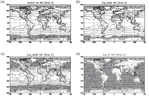
The annual mean spatial pattern of the surface air temperatures (SAT) for the control

15

run, for the experiments with prescribed surface albedo of 0.2 and 0.8, and for the ice-planet simulation are shown in Fig. 1. The grey shading indicates the sea-ice coverage. A slight decrease of the land albedo to 0.2 (Exp alb02, Fig. 1b) compared to the present day simulation (control run, Fig. 1a) leads to a global warming of around 1◦C (Table 2) and a retreat of the sea-ice margin. Especially in high latitudes, the SAT increases

20

and the sea ice retreats along the Antarctic coast. Contrary, a drastic increase of the albedo over the land to 0.8 (Fig. 1c), results in a decrease of the global annual mean SAT by about 18◦C (Table 2) and the temperature at the equator of the Atlantic Ocean is less than 15◦C (Fig. 1c). Sea-ice is formed closer to the equator as its margin reaches 40◦N and 50◦S. The experiment Exp IP shows a full Earth glaciation. The

CPD

Full Screen / Esc

Print Version Interactive Discussion

EGU global mean temperature falls to approximately −50◦C, and over Antarctica −80◦C are

reached (Fig. 1d).

The calculated globally averaged surface albedo and the planetary albedo (Table 2) show that the planetary albedo is larger by 82% and 158% than the surface albedo in the control run and Exp alb02, due to the high rates of evaporation and cloud formation.

5

In experiment Exp alb08 it is only 5%. In contrast to this, the surface albedo in the ice planet simulation (Exp IP) is larger (approximately 6%) than the planetary albedo. 3.1.2. Sensitivity of the “Ice Planet” simulations

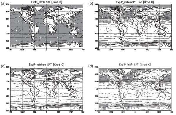
To isolate the effect and to determine the importance of each boundary and initial con-ditions, sensitivity experiments of the Ice Planet simulation are performed, holding only

10

one of the boundary conditions the same as in the case of the control run. Chang-ing the heat transport to present-day values, the model simulation does not generate any considerable change in the SAT pattern (Fig. 2a). The temperatures increase by only 0.26◦C, but the earth remains ice covered in the equilibrium state, which is reached about 5 years later than in the Exp IP (Fig. 3). If the initial temperature is

15

set to present day (AMIP) values, the planet does not end in a full glaciation, although strong sea-ice formation in the Northern Hemisphere occurs and the global tempera-ture is almost 20◦C lower compared to the control run (Table 2 and Fig. 3). Leaving the land albedo free to develop in ExpIP albfree, the global temperature increases to about 16◦C (Fig. 2c) and the spatial temperature pattern tends to resemble the control run. An

20

increase of the temperature (of about 10◦C) also occurs in the experiment ExpIP iniIP, in which the land albedo was released free to develop after 6 months of the Ice Planet integration (Figs. 2d and 3). The relation between the surface and planetary albedo in the last two sensitivity experiments is similar to the present-day conditions (the plane-tary albedo is larger than the surface albedo), characterised by an evaporation regime

25

and cloud formation (Table 2).

The decrease of temperature in the first two sensitivity experiments shows that the oceanic heat transport and the initial temperature are not sufficient to prevent the global

CPD

Full Screen / Esc

Print Version Interactive Discussion

EGU cooling. The global glaciation occurs independently of the oceanic heat transport. In

contrast to this, the increased land albedo provokes the planet’s warming and appears to be the most important factor for the change of the climate system.

3.1.3. Sensitivity of the climate system to CO₂concentration

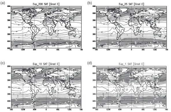
A fourfold increase of CO₂ concentration relative to present-day values, results in a

5

more than 4◦C increase of the global temperature, and a two fold increase of the CO₂ concentration provokes a 2◦C global warming (Table 2). Reduction of CO₂ to 1 ppm results in a global cooling of 25◦C compared to the control run, yielding an annual mean SAT of −7◦C in EXP 1. In Fig. 4 the SAT and the sea-ice margin evolution for experiments with CO₂concentration of 200, 25, 10 and 1 ppm are shown. Reduction

10

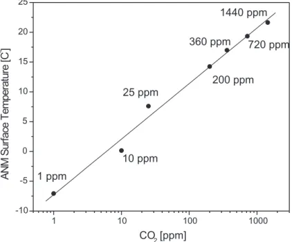
of CO₂ cools the planet, sea-ice is formed closer to the equator, and the positive ice-albedo feedback is initiated. Nevertheless, the reduction of CO₂ under present-day geography and orbital conditions is not sufficient to cause a full glaciation of the planet. The dependence of the annual mean surface temperature on the log (CO₂) shows a good linear approximation (Fig. 5) not only for the CO₂ values near the present day

15

concentration but also for the extreme concentrations as 1 ppm and 1440 ppm. 3.2. Orography and oceanic heat transport

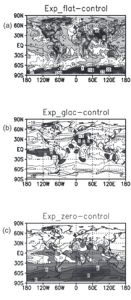
In Fig. 6 the spatial SAT pattern of the experiments investigating the role of orography and ocean heat transport are shown. Applying zero orography (EXP flat), the simula-tion shows global warming of 1◦C (Table 2). Over land, the impact is more obvious,

20

as the temperature anomaly can reach up to 8◦C in the Himalaya Massive and around 22◦C in the Antarctic (Fig. 6a). Warming also occurs over the Pacific and almost over the entire Atlantic. Still, cooling is noted in some areas of the North Atlantic and the whole Southern ocean (up to −2◦C).

The experiment forced with glacial orography (Peltier, 1994) and present-day heat

25

CPD

Full Screen / Esc

Print Version Interactive Discussion

EGU North Atlantic, and Eurasian cooling of −16◦C to −20◦C is due to the highly elevated

Laurentide Ice Sheet, influencing generally the atmospheric circulation pattern (Ro-manova et al., 2005). Along with a global cooling, an equatorial Pacific warming is found, a feature similar to that in the CLIMAP (1981) reconstruction of the Last Glacial Maximum.

5

To investigating the role of the oceanic heat transport separately, we carried out an experiment, in which all boundary conditions are set equal to those in the control run and only the ocean heat transport was reduced to zero. This experiment EXP zero shows warming in the Southern Hemisphere (SH) and cooling in the Northern Hemi-sphere (NH). This see-saw effect is due to a changed ocean heat redistribution. When

10

the meridional oceanic heat transport is prohibited, the SH warms up and the heat ex-change between the hemispheres is sharply reduced. A surplus of heat is found in the SH and a lack of it in the NH.

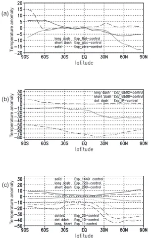
3.3. Zonal mean SAT anomalies

An overview of the zonally averaged temperature anomalies relative to the control run is

15

shown for all experiments in Fig. 7. The first panel represent the temperature anomalies for EXP glac, EXP flat and EXP zero. Strong midlatitude and polar region cooling in the NH and SH, due to the extended glacial ice sheets, is found in EXP glac. The see-saw effect between the NH and SH characterises the results of EXP zero and an overall warming except in the Southern Ocean is found in EXP flat. On the second panel

20

(Fig. 7b) the SAT anomalies for the experiments with changed albedo are displayed. EXP alb02 shows a small increase of the temperature (around 1◦C) relative to the present-day simulation, except for the Antarctic, where the sharp change of surface reflectivity from glaciers (0.8) to forest (0.2) yields a warming of nearly 10◦C; EXP alb08 exhibits strong, zonal cooling up to −30◦C in mid and high northern latitudes, indicating

25

the opposite effect than in EXP alb02 for the Antarctic; and in EXP IP the temperature anomaly can reach −70◦C in the equatorial and tropical latitudes. The third panel visualizes the temperature reduction in the NH due to the reduction of CO₂ and the

CPD

Full Screen / Esc

Print Version Interactive Discussion

EGU consequential positive ice-albedo feedback. The extreme experiment EXP 1 exhibits

very strong anomalies, up to −40◦C SAT in the subtropics in the NH. 3.4. Zonal mean precipitation

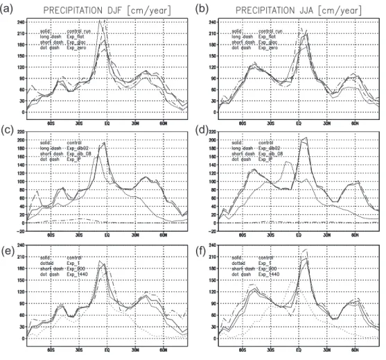
To assess the Hadley circulation and the Intertropical Convergence Zone (ITCZ) for dif-ferent sensitivity experiments the averaged zonal mean precipitation is calculated. The

5

zonal mean boreal winter and summer values for the sensitivity experiments are shown in Fig. 8. The maximum precipitation in boreal winter for the present-day simulation is situated in the SH, while in the boreal summer it is located in the NH.

The experiments investigating the effect of the orography (Figs. 8a and 8b) EXP flat and EXP glac show seasonal deviations from the present-day values. In EXP flat the

10

maximum precipitation during boreal winter is reduced, while in EXP glac it is en-hanced. The opposite tendency is found in boreal summer, EXP flat shows an increase in precipitation and experiment EXP glac produces a decrease. The land elevation in the NH results in pronounced seasonality in the equatorial region. As the orography is higher, the ITCZ is strengthened in boreal winter and is suppressed in boreal summer.

15

The absence of heat transport in EXP zero increases the maximum precipitation in both seasons, compared to the control run.

The precipitation in the land albedo experiment EXP alb02 is similar to the present-day’s one, except in the region of Antarctica, where the drastic change of the albedo produces a peak in precipitation in winter (Figs. 8c and 8d). In EXP alb08 the

precip-20

itation maximum is strongly shifted to the SH (around 15◦S) and located in the belt of all-years SAT maximum. The magnitude is 20% less than the present-day value. A decrease in precipitation occurs in the midlatitudes of the NH and SH due to the extensive ice-coverage and negative surface temperatures. The ice-covered planet in EXP IP prohibits precipitation the whole year round.

25

The experiment with a fourfold present-day CO₂concentration shows a decrease in the precipitation during boreal winter and an increase during boreal summer (Figs. 8e and 8f). The tendency is the same as in EXP flat (described earlier), whereas the

ex-CPD

Full Screen / Esc

Print Version Interactive Discussion

EGU periment with CO₂equal to 200 ppm exhibits the tendency of EXP glac – an increase in

the precipitation during boreal winter and decrease during boreal summer. Therefore, glacial orography and the reduction of CO₂act in the same direction. Both change the ITCZ and Hadley circulation in equatorial and tropical latitudes. In experiment EXP 1 the precipitation is considerably lowered, as its maximum does not experience

season-5

ality and is always located in the SH, tending to the same result as in EXP alb08.

4. Discussions

Motivated by recent attempts to simulate Neoproterozoic glaciations with climate mod-els (e.g. Jenkins and Smith, 1999; Hyde at al., 2000; Chandler and Sohl, 2000; Poulsen et al., 2001; Lewis et al., 2003; Donnadieu et al., 2004), we investigate the sensitivity

10

of the climate to some extreme boundary and initial conditions and combinations of extreme parameters under present-day insolation and continental distributions. Exam-ining the influence of each factor, we assess the role of the land albedo, the influence of high and low CO₂concentration levels, the importance of the orography and of the oceanic heat transport.

15

The experiments with only one parameter changed, show equilibrium states, in which the equatorial ocean remains ice-free. Using a combination of extreme boundary and initial conditions, like zero oceanic heat transport, high land albedo and the initial tem-perature uniformly set to a value equal to the freezing point, an ice-covered Earth under present-day orbital parameters and CO₂concentration can be attained. Further

20

investigation of the experiments with a combination of two of the mentioned extreme boundary conditions, shows that the dominant factor for the decrease of temperature in the ice planet simulation is the land albedo. If the land albedo is a variable parameter, independently of the zero oceanic heat transport or the low initial temperature field, the temperatures increase and tend to reach the values of the control run. Interestingly,

25

the present-day oceanic heat transport alone is not able to produce ice-free equatorial oceans. A full glaciation is delayed but successfully reaches the ice-planet equilibrium

CPD

Full Screen / Esc

Print Version Interactive Discussion

EGU (Fig. 3). Even though the heat transport of the present-day climate seems not to be

ap-propriate with respect to ice-covered oceans (Poulsen et al., 2001; Lewis et al., 2003), its role appears to be negligible compared to continental surface properties. Using a 2,5 dimensional coupled climate model of intermediate complexity, Dounadieu et al. (2004) concluded that the dynamic oceanic process cannot prevent the onset of the

5

ice-albedo instability in a Neoproterozoic simulation. Another factor prohibiting the for-mation of an ice-covered planet is the high initial temperature field (set to present-day values). Although the global temperature falls approximately 20◦C, the sea-ice cover advance is restricted up to 30◦N and 60◦S. The asymmetrical distribution of the sea-ice margins is more sensitive to the paleogeography differences than to the change of

10

other parameters, e.g. the insolation (Poulsen et al., 2002). Releasing the land albedo after the 20-th year of the ice planet simulation (not shown) does not infer any change in the climate system, due to the very low temperatures, which force the land and ice albedo to attain their maximal values. Thus, the ice planet simulation reaches a stable climate and only an external influence can lead to change of this stable state

15

(e.g. increase of carbon dioxide due to strong volcanic activity and lack of chemical weathering).

Does the orography matter in the initiation of extreme climate? The LGM reconstruc-tion of the orography (Peltier, 1994), including the highly elevated Laurentide Ice Sheet, reduces the global temperature by 3◦C. The influence of changed orography

predomi-20

nates in the contribution to the Northern Hemispheric cooling, but it is of no importance to the tropics. Thus the altered orography is more important in regional sense, than in global. Jenkins and Frakes (1998) introduced a 2 km north-south mountain chain on the super continent in their Neoproterozoic model set up, and showed that the orogeny could not be considered as a factor for the global glaciation. But it can redistribute the

25

humidity over sea-ice and thus, change the hydrological cycle (Donnadieu et al., 2003). However, the climate system responses nonlinearly to linear change of the height of the ice-sheet (Romanova et al., 2005), which points to the existence of a threshold, over which a runaway albedo feedback over the American continent could be initiated.

CPD

Full Screen / Esc

Print Version Interactive Discussion

EGU Further investigation of the sensitivity of the climate system toward enlargement of the

Laurentide Ice Sheet could be of interest when searching for this threshold.

The experiments control run, EXP alb02, EXP flat, EXP 1440 showed a planetary albedo larger than the surface albedo (in some cases more than 150%), due to the strong evaporation over the ice-free oceans and cloud formation. In the experiments

5

(EXP alb08, EXPIP iniTempPD and EXP 1), in which the absolute global temperature is around 0◦C and which are characterised by cold climatic conditions and ice-free equatorial and tropical latitudes, the global surface and planetary albedo tend to be in the same order. However, these cold climates (EXP alb08 and EXP 1) could exhibit an intense equatorial precipitation maxima and a strong Hadley circulation due to the

10

sharp temperature gradients from the equator to the edge of the sea-ice margin, which works against the positive ice-albedo feedback (Bendtsen, 2002). The hydrological cycle and the ITCZ are rather sensitive to the change of the surface temperature in the tropics and to the strength of the Atlantic overturning (Lohmann and Lorenz, 2000; Lohmann, 2003). Interestingly, in the ice-planet experiments EXP IP and EXPIP iniIP,

15

the estimates of the global planetary albedo appear smaller than the global surface albedo. On a completely glaciated Earth, the processes of evaporation, cloud formation and precipitation are strongly suppressed or even do not exist, thus the ratio between the incident and reflected short wave radiation on the surface is higher than the ratio between the incident and reflected/scattered short wave radiation on the top of the

20

atmosphere. The loss of energy in the atmosphere could be due to the process of water vapour absorption, where the water vapour is provided only by the process of sublimation.

5. Concluding remarks

Motivated by the early work with EBMs (Budyko, 1969; Sellers, 1969) and the

discus-25

sion about an ice covered Earth (e.g. Crowley and Baum, 1993; Jenkins and Frakes, 1998; Hyde et al., 2000; Chandler and Sohl, 2000; Crowley et al., 2001; Poulsen et al.,

CPD

Full Screen / Esc

Print Version Interactive Discussion

EGU 2001; Donnadieu et al., 2002; Bendtsen, 2002; Lewis et al., 2003; Donnadieu et al.,

2004; Stone and Yao, 2004), we investigate the possibility for extreme climates under present configurations (continent distribution and orbital forcing) in a simplified AGCM coupled to a mixed layer-sea ice model (Fraedrich, 1998; Franzke et al., 2000; Grosfeld et al., 20052; Romanova et al. 2005).

5

Investigating the Neoproterozoic glaciations, many authors search for a CO₂ thresh-old value. Different simulations show a sensitivity of the minimum CO₂ level to con-tinental configurations (Poulsen et al., 2002; Donnadieu et al., 2004), Earth’s rotation rate and obliquity (Jenkins and Smith, 1999; Jenkins, 2000), solar luminosity (Crow-ley et al., 2001) oceanic heat transport (Poulsen et al., 2001) or an increase of the

10

albedo (Lewis et al., 2003). Our experiments for present day setup suggest that the reduction of atmospheric CO₂alone is not sufficient to provoke global glaciation under present-day insolation. We find a strong nonlinearity in the NH at a CO₂ concentra-tion of 25 ppm. The temperature anomaly, relative to the present-day simulaconcentra-tion, can reach −40◦C at 1 ppm. Our simulations show that the initial condition of the system is

15

important when simulating a snowball Earth. Indeed, a hysteresis of the climate sys-tem is found with respect to a change of the infrared forcing (Crowley et al., 2001) and solar constant (Stone and Yao, 2004). We suppose similar climate behaviour to a slow change of the CO₂ concentration and a snow cover and we will address this question in our further research.

20

In our sensitivity experiments we evaluated extreme effects of land albedo and CO₂ on climate in a similar way as Fraedrich et al. (1999) for vegetation extremes on the at-mosphere. In our approach, we calculated the sea surface temperature interactively by assuming different ocean heat transports. We have neglected several climatic links be-tween the components, including e.g. the hydrological cycle/temperature, vegetation,

25

weathering rates, carbon cycle, and deep ocean circulation. As a logical next step, 2

Grosfeld, K., Lohmann, G., Rimbu, N., Lunkeit, F., and Fraedrich, K.: Signature of atmo-spheric multidecadal variations in the North Atlantic realm as derived from proxy data, obser-vations, and model studies, Int. J. Climatol., submitted, 2005.

CPD

Full Screen / Esc

Print Version Interactive Discussion

EGU more interactive climate components will be included in order to estimate the most

extreme climate states under present and past climate configurations. The combined effects yield different regimes which are relevant to understand past climate evolutions as recorded, e.g. in cabonate deposites.

Acknowledgements. We gratefully acknowledge the suggestions and recommendations of

5

F. Lunkeit and thank K. Fraedrich for providing us with the model code. We thank also M. Dima and K. Vosbeck for the improvement of the manuscript. This work has been funded by the Ger-man Ministry for Education and Research (BMBF) within DEKLIM project “Climate Transitions” and MARCOPLI.

References

10

Bendtsen, J.: Climate sensitivity to changes in solar insolation in a simple coupled model, Clim. Dyn., 18, 595–609, 2002.

Berger, A. L.: Long term variations of daily insolation and quaternary climatic changes, J. Atmos. Sci., 35, 2362—2367, 1978

Budyko, M. I.: The effect of solar radiation variations on the climate of the Earth, Tellus, 21,

15

611–619, 1969.

Butzin, M., Prange, M., and Lohmann, G.: Studien zur 14C-Verteilung im glazialen Ozean mit einem globalen Ozeanzirkulationsmodell, Terra Nostra, 6, 86–88, 2003.

Butzin, M., Prange, M., and Lohmann G.: Radiocarbon simulations for the glacial ocean: the effects of wind stress, Southern Ocean sea ice and Heinrich events, Earth Planet. Sci. Lett.,

20

235, 45-61, doi:10.1016/j.epsl.2005.03.003, 2005.

Chandler, M. A. and Sohl, L. E.: Climate forcings and the initiation of low-latitude ice sheets dur-ing Neoproterozoic Varanger glacial interval, J. Geophys. Res., 105, 20 737–20 756, 2000. Claussen, M., Mysak, L. A., Weaver, A. J., Crucifix, M., Fichefet, T., Loutre, M. F., Weber, S.L.,

Alcamo, J., Alexeev, V. A., Berger, A., Calov, R., Ganopolski, A., Goosse, H., Lohmann, G.,

25

Lunkeit, F., Mokhov, I. I., Petoukhov, V., Stone, P., and Wang, Z.: Earth system models of intermediate complexity: Closing the gap in the spectrum of climate system models, Clim. Dyn., 18, 579–586, 2002.

CPD

Full Screen / Esc

Print Version Interactive Discussion

EGU

Maximum, Geological Society of America, Map and Chart Series, MC-36, 18, 18 maps, 1981.

Crowley, T. J. and Baum, S. K.: Effects of decreased solar luminosity on Late Precambrian ice extent, J. Geophys. Res., 98, 16723–16732, 1993.

Crowley, T. J., Hyde, W. T., and Peltier, W. R.: CO₂levels required for deglaciation of a “Near

5

Snowball” Earth, Geophys. Res. Lett., 28, 283–286, 2001.

Donnadieu, Y., Ramstein, G., Fluteau, F., Besse, J., and Meert, J.: Is high obliquity a plausible cause for Neproterozoic glaciations?, Geophys. Res. Lett., 29, doi:10.1029/2002GL015902, 2002.

Donnadieu, Y., Fluteau, F., Ramstein, G., Ritz, C., and Besse, J.: Is there a conflict between

10

the Neoproterozoic glacial deposits and snowball Earth interpretation: an improved under-standing with numerical modeling, Earth Plan. Sci. Lett., 208, 101–112, 2003.

Donnadieu, Y., Ramstein, G., Fluteau, F., Roche, D., and Ganopolski, A.: The impact of atmo-spheric and oceanic heat transports on the sea-ice-albedo instability during the Neoprotero-zoic, Clim. Dyn., 22, 293–306, 2004

15

Eliasen, E., Machenhauer, B., and Rasmussen, E.: On a numerical method for integration of the hydrodynamical equations with a spectral representation of the horizontal fields, Report No. 2, Institute for Theoretical Meteorology, University of Copenhagen, 37 pp., 1970. Evans, D. A. D., Li, Z. X., Kirschvink, J. L., and Wingate, M. T. D.: A high-quality

mid-Neoproterozoic paleomagnetic pole from South China, with implications for ice ages and

20

the breakup configuration of Rodinia, Precambrian Res., 100, 313–334, 2000.

Fraedrich, K., Kirk, E., and Lunkeit, F.: Portable University Model of the Atmosphere, Deutsches Klimarechenzentrum, Tech. Rep., 16, 377 pp., 1998.

Fraedrich, K., Kleidon, A., and Lunkeit, F.: A green planet versus a desert world: Estimating the effect of vegetation extremes on the atmosphere, J. Climate, 12, 3156–3163, 1999.

25

Franzke, C., Fraedrich, K., and Lunkeit, F.: Low frequency variability in a simplified atmospheric global circulation model: Storm track induced “spatial resonance”, Quat. J. Roy. Met. Soc. 126, 2691–2708, 2000.

Frisius, T., Lunkeit, F., Fraedrich, K., and James, I. N.: Storm-track organization and variability in a simplified atmospheric global circulation model (SGCM), Quat. J. Roy. Met. Soc., 124,

30

1019–1043, 1998.

Hoffman, P. F. and Schrag, D. P.: The snowball Earth hypothesis: testing the limits of global change, Terra Nova, 14, 129–155, 2002.

CPD

Full Screen / Esc

Print Version Interactive Discussion

EGU

Hoffman, P. F., Kaufman, A. J., Halverson, G. P., and Scharg, D. P.: A Neoproterozoic snowball earth, Science, 281, 1342–1346, 1998.

Hyde, W. T., Crowley, T. J., Baum, S. K., Peltier, W. R.: Neoproterozoic “snowball Earth” simu-lations with a coupled climate/ice-sheet model, Nature, 405, 425–429, 2000.

Jenkins, G. S.: Global climate model high-obliquity solutions to the ancient climate puzzles of

5

the Faint Young Sun Paradox and low altitude Proterozoic Glaciation, J. Geophys. Res., 105, 7357–7370, 2000.

Jenkins, G. S. and Frakes, L. A.: GCM sensitivity test using increased rotation rate, reduced so-lar forcing and orography to examine low latitude glaciation in the Neoproterozoic, Geophys. Res. Lett., 25, 3525–3528, 1998.

10

Jenkins, G. S. and Smith, S. R.: GCM simulation of Snowball Earth conditions during the late Proterozoic, Geophys. Res. Lett., 26, 2263–2266, 1999.

Kirschvink, J. L.: Late proterozoic low-lattitude global glaciation: the Snowball Earth, in: The Proterozoic biosphere, edited by: Schopf, J. W. and Klein, C., Cambridge UK, 51–52, 1992. Kirschvink, J. L., Gaidos, E. J., Bertani, E., Beukes, N. J., Gutzmer, J., Maepa, L. N., and

15

Steinberger, R. E.: Paleoproterozoic snowball Earth: Extreme climatic and geochemical global change and its biological consequences, PNAS, 97, 1400–14005, 2000.

Kleidon, A., Fraedrich, K., and Heimann, M.: A green planet versus a desert world: Estimating the maximum effect of vegetation on the surface energy balance, Climatic Change, 44, 471– 493, 2000.

20

Kubatzki, C. and Claussen M.: Simulation of the global bio-geophysical interactions during the Last Glacial Maximum, Climate Dynamics, 14, 461–471, 1998.

Langen, P. L. and Alexeev, V. A.: Multiple equilibria and asymmetric climates in the CCM3 coupled to an oceanic mixed layer with thermodynamic sea ice, Geophys. Res. Lett., L04201, doi:10.1029/2003GL019039, 2004.

25

Lewis, J. P., Weaver, A. J., Johnston, S. T., and Eby, M.: Neoproterozoic “snowball Earth”: Dy-namic sea ice over a quiescent ocean, Paleoceanography, 18, doi:10.1029/2003PA000926, 2003.

Lohmann, G.: Atmospheric and oceanic freshwater transport during weak Atlantic overturning circulation, Tellus, 55A, 438–449, 2003.

30

Lohmann, G. and Lorenz, S.: On the hydrological cycle under paleoclimatic conditions as derived from AGCM simulations, J. Geophys. Res., 105, 417–436, 2000.

conti-CPD

Full Screen / Esc

Print Version Interactive Discussion

EGU

nental configuration and of the seasonal cycle on the climatic stability, Glob. Plan. Change, 14, 97–112, 1997.

Lorenz, S., Grieger, B., Helbig, Ph., and Herterich K.: Investigating the sensitivity of the at-mospheric general circulation model ECHAM 3 to paleoclimatic boundary conditions, Geol. Rundsch. 85, 513-524, 1996.

5

Lunkeit, F., Bauer, S. E., and Fraedrich, K.: Storm tracks in a warmer climate: Sensitivity studies with a simplified global circulation model, Clim. Dyn., 14, 813–826, 1998.

Macdonald, A. M., and Wunsch, C.: An estimate of global ocean circulation and heat fluxes, Nature, 382, 436–439, 1996.

Orszag, S. A.: Transform method for calculation of vector-coupled sums: Application to the

10

spectral form of the vorticity equation, J. Atmos. Sci., 27, 890–895, 1970. Peltier, W. R.: Ice age paleotopography, Science, 265, 195–201, 1994.

Phillips, T. J., Anderson, R., and Br ¨osius, M.: Hypertext summary documentation of the AMIP models, UCRL-MI-116384, Lawrence Livermore National Laboratory, Livermore, CA, 1995. Poulsen, C. J., Pirrehumbert, R. T., and Jacob, R. L.: Impact of ocean dynamics on the

simula-15

tion of the Neoproterozoic “snowball Earth”, Geophys. Res. Lett., 28, 1575–1578, 2001. Poulsen, C. J., Jacob, R. L., Pierrehumbert, R. T., and Huynh, T. T.: Testing

pale-ogeographic controls on a Neoproterozoic snowball Earth, Geophys. Res. Lett., 29, doi:10.1029/2001GL014352, 2002.

Poulsen, C. J.: Absence of runaway ice-albedo feedback in the Neoproterozoic, Geology, 31,

20

473–476, 2003.

Roeckner, E., Arpe, K., Bengtsson, L., Brinkop, S., D ¨umenil, L., Esch, M., Kirk, E., Lunkeit, F., Ponater, M., Rockel, B., Sausen, R., Schlese, U., Schubert, S., and Windelband, M.: Simula-tion of present-day climate with the ECHAM model: Impact of model physics and resoluSimula-tion, MPI Report No. 93, ISSN 0937-1060, Max-Planck-Institut f ¨ur Meteorologie, Hamburg,

Ger-25

many, 171 pp., 1992.

Romanova, V., Lohmann, G., Grosfeld, K., and Butzin, M.: The relative role of oceanic heat transport and orography on glacial climate, Quat. Sci. Rev., in press, 2005.

Schmidt, P. W. and Williams, G. E.: The Neoproterozoic climatic paradox; equatorial palaeolat-itude for Marinoan Glaciation near sea level in South Australia, Earth Planet. Sci. Lett., 134,

30

107–124, 1995.

Sellers, W. D.: A climate model based on the energy balance of the earth atmosphere system, J. Appl. Meteorol., 8, 392–400, 1996.

CPD

Full Screen / Esc

Print Version Interactive Discussion

EGU

Sohl, L. E., Christie-Blick, N., and Kent, D. V.: Paleomagnetic polarity reversals in Marinoan (ca. 600 Ma) glacial deposits of Australia: implications for the duration of low-latitude glaciation in Neoproterozoic time, Geol. Soc. Am. Bull., 111, 8, 1120–1139, 1999.

Stone, P. H. and Yao, M. S.: The ice-covered Earth instability in a model of intermediate com-plexity, Clim. Dyn., doi:10.1007/s00382-004-0408-y, 2004.

5

Wyputta, U. and McAvaney, B. J.: Influence of vegetation changes during the Last Glacial Maximum using the BMRC atmospheric general circulation model, Clim. Dyn., 17, 923–932, 2001.

CPD

Full Screen / Esc

Print Version Interactive Discussion

EGU Table 1. Overview of numerical experiments and their set-up.

Sensitivity experiments CO2 Orography Abbreviation

AMIP (prescribed at the surface) 360 Present-day Exp_prescr

10 years averaged surface heat fluxes from exp. Exp_prescr

360 Present-day Exp_slab

(control run)

Albedo albedo land -0.2

albedo ocean -0.069 Exp_alb02

albedo land -0.8

albedo ocean -0.069 Exp_alb08

albedo land: 0.8 initial temp: -1.9°C heat transport: zero

360 Present-day Exp_IP (ice-planet) albedo land: 0.8 initial temp: -1.9°C heat transport: PD ExpIP_HfPD albedo land: 0.8 initial temp: PD

heat transport: zero

ExpIP_iniTempPD

albedo land: free

initial temp: -1.9°C heat transport: zero

ExpIP_albfree Sensitivity toward initial and boundary conditions

Initial state Exp_IP Albedo land: free Heat transport: zero

360 Present-day ExpIP_iniIP CO2 – 1 ppm 1 Present-day Exp_1 CO2 - 10 ppm 10 Present-day Exp_10 CO2 - 25 ppm 25 Present-day Exp_25 CO2 - 200 ppm 200 Present-day Exp_200 CO2 - 720 ppm 720 Present-day Exp_720 CO2 - 1440 ppm 1440 Present-day Exp_1440

Zero orography 360 Zero Exp_flat

Glacial orography 360 (Peltier 1994) Exp_glac

CPD

Full Screen / Esc

Print Version Interactive Discussion

EGU Table 2. Annual mean, DJF and JJA surface air temperatures (SAT) and globally averaged

surface and planetary albedo.

Global Temperature (ºC) Exp. name ANM DJF JJA

Planetary Albedo (in fraction) Surface Albedo (in fraction) control 17.00 15.84 18.36 0.31 0.17 Exp_alb02 18.33 17.21 19.65 0.31 0.12 Exp_alb08 -0.36 -1.26 1.10 0.41 0.39 Exp_IP -50.58 -49.20 -52.11 0.69 0.73 ExpIP_HfPD -50.84 -49.61 -52.23 0.69 0.73 ExpIP_iniTempPD -1.02 -2.76 1.21 0.42 0.38 ExpIP_albfree 16.14 14.66 17.15 0.32 0.18 ExpIP_iniIP 2.94 1.23 5.17 0.39 0.33 Exp_1 -6.75 -6.73 -6.76 0.40 0.39 Exp_10 0.15 -0.50 1.35 0.37 0.33 Exp_25 7.61 6.84 8.97 0.33 0.26 Exp_200 14.25 13.03 15.85 0.32 0.20 Exp_720 19.35 18.20 20.76 0.32 0.15 Exp_1440 21.64 20.54 22.99 0.32 0.13 Exp_glac 13.96 12.54 15.80 0.33 0.23 Exp_flat 18.23 17.02 19.70 0.31 0.16 Exp_zero 16.19 14.75 17.96 0.32 0.17

CPD

Full Screen / Esc

Print Version Interactive Discussion EGU (a) (b) (c) (d) Fig. 1

Fig. 1. Spatial pattern of the annual mean surface air temperatures averaged over a period of

25 years of integration for experiments(a) control run; (b) Exp alb02; (c) Exp alb08; and (d)

Exp IP (land alb. set to 0.8; initial temp. set to −1.9◦C; the oceanic heat transport is zero). The grey shading indicates the annual mean sea-ice cover.

CPD

Full Screen / Esc

Print Version Interactive Discussion EGU (a) (b) (c) (d) Fig. 2

Fig. 2. As in Fig. 1, but for experiments (a) ExpIP HfPD (PD heat transport); (b)

Ex-pIP iniTempPD (Pd initial temperature);(c) ExpIP albfree (land alb. simulated by the model);

and(d) ExpIP iniIP (land alb. – 0.6; zero heat transp.; initial temp. −1.9◦C; after six months the albedo is released to develop).

CPD

Full Screen / Esc

Print Version Interactive Discussion

EGU Fig. 3

Fig. 3. Time series of global average surface temperature for ExpIP HfPD, ExpIP iniTempPD,

CPD

Full Screen / Esc

Print Version Interactive Discussion EGU (a) (b) (c) (d) Fig. 4

Fig. 4. As in Fig. 1, but for experiments (a) Exp 200; (b) Exp 25; (c) Exp 10; and (d) Exp 1.

CPD

Full Screen / Esc

Print Version Interactive Discussion EGU 1 10 100 1000 -10 -5 0 5 10 15 20 25 1 ppm 10 ppm 1440 ppm 720 ppm 200 ppm 25 ppm 360 ppm A N M S ur fa ce Tem per at ur e [C º ] CO₂[ppm] Fig. 5

Fig. 5. Log plot of the carbon dioxide concentration versus ANM surface temperature for exp.

Exp 1, Exp 10, Exp 25, Exp 200, Exp 360, Exp 720 and Exp 1440. The line shows the linear fit.

CPD

Full Screen / Esc

Print Version Interactive Discussion EGU (a) (c) (b) Fig. 6

Fig. 6. Annual mean surface air temperatures anomalies: (a) Exp flat-control run (zero

orogra-phy);(b) Exp glac-control run (LGM orography given by Peltier, 1981); and (c) Exp zero-control

CPD

Full Screen / Esc

Print Version Interactive Discussion EGU (a) (c) (b) Fig. 7 Temperature anomaly Temperature anomaly Temperature anomaly

Fig. 7. Zonal mean of the global surface temperature anomalies relative to the control run: (a) effect of orography and oceanic heat transport; (b) changed land albedo and Ice Planet

CPD

Full Screen / Esc

Print Version Interactive Discussion EGU (a) (e) (c) Fig. 8 (b) (f) (d)

Fig. 8. The DJF and JJA zonal mean precipitation for control run (solid line) and (a), (b) the

ex-periments investigating the effect of orography and oceanic heat transport; (c), (d) experiments with changed land albedo and Ice Planet simulation; and(e), (f) experiments with different CO2