HAL Id: hal-01700238
https://hal.archives-ouvertes.fr/hal-01700238
Submitted on 31 Aug 2018
HAL is a multi-disciplinary open access
archive for the deposit and dissemination of
sci-entific research documents, whether they are
pub-lished or not. The documents may come from
teaching and research institutions in France or
abroad, or from public or private research centers.
L’archive ouverte pluridisciplinaire HAL, est
destinée au dépôt et à la diffusion de documents
scientifiques de niveau recherche, publiés ou non,
émanant des établissements d’enseignement et de
recherche français ou étrangers, des laboratoires
publics ou privés.
Star formation history from the cosmic infrared
background anisotropies
A. Maniyar, M. Béthermin, Guilaine Lagache
To cite this version:
A. Maniyar, M. Béthermin, Guilaine Lagache. Star formation history from the cosmic infrared
background anisotropies. Astronomy and Astrophysics - A&A, EDP Sciences, 2018, 614 (A39),
�10.1051/0004-6361/201732499�. �hal-01700238�
March 17, 2018
Star formation history from the cosmic infrared background
anisotropies
A. S. Maniyar, M. Béthermin, and G. Lagache
Aix-Marseille Université, CNRS, LAM, Laboratoire d’Astrophysique de Marseille, Marseille, France e-mail: abhishek.maniyar@lam.fr
Received 19 December 2017 / Accepted 29 January 2018
ABSTRACT
We present a linear clustering model of cosmic infrared background (CIB) anisotropies at large scales that is used to measure the cosmic star formation rate density up to redshift 6, the effective bias of the CIB, and the mass of dark matter halos hosting dusty star-forming galaxies. This is achieved using the Planck CIB auto- and cross-power spectra (between different frequencies) and CIB × CMB (cosmic microwave background) lensing cross-spectra measurements, as well as external constraints (e.g. on the CIB mean brightness). We recovered an obscured star formation history which agrees well with the values derived from infrared deep surveys and we confirm that the obscured star formation dominates the unobscured formation up to at least z= 4. The obscured and unobscured star formation rate densities are compatible at 1σ at z= 5. We also determined the evolution of the effective bias of the galaxies emitting the CIB and found a rapid increase from ∼0.8 at z= 0 to ∼8 at z = 4. At 2 < z < 4, this effective bias is similar to that of galaxies at the knee of the mass functions and submillimetre galaxies. This effective bias is the weighted average of the true bias with the corresponding emissivity of the galaxies. The halo mass corresponding to this bias is thus not exactly the mass contributing the most to the star formation density. Correcting for this, we obtained a value of log(Mh/M )= 12.77+0.128−0.125for the mass of the typical dark matter halo contributing to the CIB at z= 2. Finally, using a Fisher matrix analysis we also computed how the uncertainties on the cosmological parameters affect the recovered CIB model parameters, and find that the effect is negligible.
Key words. galaxies: evolution – galaxies: star formation – galaxies: halos – cosmology: observations – methods: statistical
1. Introduction
1
How and when the galaxies assembled their stars are two of
2
the most pressing questions of modern cosmology. In the last
3
decade, it has become clear that the dusty star-forming galaxies
4
are significant contributors to this process as they pin down the
5
episodes of galaxy-scale star formation (e.g.Gispert et al. 2000;
6
Casey et al. 2014). Indeed they are a critical player in the
assem-7
bly of stellar mass and the evolution of massive galaxies (e.g.
8
Béthermin et al. 2015).
9
Dusty star-forming galaxies are difficult to detect
individ-10
ually at high redshift because they are so faint and numerous
11
compared to the angular resolution achievable in the far-infrared
12
to millimetre wavelengths that the confusion limits the
ulti-13
mate sensitivity (e.g. Nguyen et al. 2010). As a result,
single-14
dish experiments, such as Herschel and Planck, can only see
15
the brightest objects that represent the tip of the iceberg in
16
terms of star formation rates and halo masses. These
experi-17
ments are nevertheless sensitive enough to measure the cosmic
18
infrared background (CIB), the cumulative infrared emission
19
from all galaxies throughout cosmic history (Lagache et al. 20
2005;Planck Collaboration XVIII 2011). The mean value of the
21
CIB gives the amount of energy released by the star
forma-22
tion that has been reprocessed by dust (Dole et al. 2006), while
23
CIB anisotropies trace the large-scale distribution of dusty
star-24
forming galaxies, and can thus be used to trace the underlying
25
distribution of the dark matter halos in which such galaxies
26
reside (Amblard et al. 2011;Viero et al. 2013;Béthermin et al. 27
2013;Planck Collaboration XXX 2014b).
28
The cosmic history of star formation is one of the most 29
fundamental observables in astrophysical cosmology. A con- 30
sistent picture has emerged in recent years, whereby the star- 31
formation rate density peaks at z ∼ 2, and declines exponentially 32
at lower redshift. The Universe was much more active in form- 33
ing stars in the past; the star formation rate density was about 34
ten times higher at z ∼ 2 than is seen today (Madau & Dickinson 35 2014). These highest star formation rate densities are the conse- 36
quence of the rising contribution from the dusty star formation. 37
At higher redshift (z 2), the level of dust-obscured star forma- 38
tion density is still a matter of debate; there is no census for the 39
star formation rate density (SFRD) selected from dust emission 40
alone (e.g.Koprowski et al. 2017). With their unmatched redshift 41
depth, CIB anisotropies can be used to improve our understand- 42
ing of early star formation. The contribution of dusty galaxies to 43
the SFRD can be derived from their mean emissivity per comov- 44
ing unit volume as derived from CIB anisotropy modelling. This 45
has been investigated byPlanck Collaboration XXX(2014b). In 46
this paper, we revisit this determination using Planck CIB mea- 47
surements combined with the latest observational constraints and 48
theoretical developments. 49
Galaxy clustering is another piece of information embedded 50
into the CIB anisotropies (Knox et al. 2001;Lagache et al. 2007). 51
The distribution of galaxies is known to be biased relative to 52
that of the dark matter. In the simplest model, on large scales, 53
it is assumed that the galaxy and dark matter mass–density fluc- 54
tuations are related through a constant bias factor b such that 55
(∆ρ/ρ)light = b(∆ρ/ρ)mass. Light traces mass exactly if b = 1 56
larger than the individual galaxy halos); if b > 1, light is a biased
1
tracer of mass, as expected if the galaxies form in the highest
2
peaks of the density field. The galaxy bias is dependent on the
3
host dark matter halo mass and the redshift (Mo & White 1996).
4
As expected by theory (e.g.Kaiser 1986;Wechsler et al. 1998)
5
and confirmed by observations (e.g.Adelberger et al. 2005), the
6
biasing becomes more pronounced at high redshift. As most of
7
the star formation over the history of the Universe has been
8
obscured by dust (Dole et al. 2006), studying the clustering of
9
dusty galaxies is crucial to exploring the link between dark
mat-10
ter halo mass and star formation. Measurements of correlation
11
function of individually resolved galaxies, whilst not forming the
12
dominant contribution to the CIB, give constraints on the host
13
halo mass of the brightest star-forming objects, the submillimetre
14
galaxies (SMGs).Maddox et al.(2010) andCooray et al.(2010)
15
measured the correlation function of Herschel/SPIRE galaxies
16
(see also Weiß et al. 2009; Williams et al. 2011 for
measure-17
ments from ground-based observations), but their results were
18
inconsistent probably because of the difficulty in building
well-19
controlled selections in low angular resolution data (Cowley 20
et al. 2016). One way to get more accurate measurements is to use
21
the cross-correlation with optical/near-IR samples (Hickox et al. 22
2012;Béthermin et al. 2014;Wilkinson et al. 2017). These
anal-23
yses found the host halo mass of galaxies with the star formation
24
rate (SFR) > 100 M to be ∼1012.5−13M . Reaching the
popu-25
lation that contributes to the bulk of the CIB requires modelling
26
the angular power spectrum of CIB. Making various assumptions
27
such as the form of the relationship between galaxy luminosity
28
and halo mass, a typical halo mass for galaxies that dominate the
29
CIB power spectrum has been found to lie between 1012.1±0.5M
30
and 1012.6±0.1M
(Viero et al. 2013;Planck Collaboration XXX
31
2014b). In this paper, we exploit the strength of Planck, which
32
is a unique probe of the large-scale anisotropies of the CIB. We
33
use only the linear part of the power spectra, and thus consider
34
a simple model (with few parameters), to measure the galaxy
35
clustering of dusty star-forming galaxies up to z ∼ 5.
36
All previous CIB angular power spectrum analyses have
con-37
sidered a fixed cosmology. Assuming a cosmology is a fair
38
assumption as the model of the CIB galaxy properties has
39
far greater uncertainties than on the cosmological parameters
40
(Planck Collaboration XIII 2016b). However, the CIB power
41
spectrum depends on key cosmological ingredients, such as the
42
dark matter power spectrum, cosmological distances, and
cos-43
mological energy densities. Therefore, it is worth studying the
44
impact of the cosmology on CIB modelling parameters, which
45
we do here for the first time.
46
The paper is organised as follows. We describe the CIB
47
anisotropy modelling and the data we use to constrain the model
48
in Sect.2. In Sect.3, we present and discuss the redshift
distribu-49
tion of CIB anisotropies and mean level, and the star formation
50
rate density from z= 0 to z = 6 that are obtained by fitting our
51
model to the CIB and CIB × CMB lensing power spectra
mea-52
surements and by using extra constraints coming from galaxy
53
number counts and luminosity functions. We then discuss the
54
host dark matter halo mass of CIB galaxies in Sect. 4 by first
55
measuring the effective bias beff, then converting it to the mean
56
bias of halos hosting the dusty galaxies, before finally
comput-57
ing the host dark matter halo mass of the dusty star formation.
58
In Sect. 5, we study the effect of cosmology on the CIB. We
59
conclude in Sect.6.
60
Throughout the paper, we used a Chabrier mass function
61
(Chabrier 2003) and the Planck 2015 flat ΛCDM
cosmol-62
ogy (Planck Collaboration XIII 2016b) with Ωm = 0.33 and
63
H0= 67.47 km s−1Mpc−1.
64
2. CIB modelling on large scales 65
2.1. CIB power spectrum 66
The measured CIB intensity Iν at a given frequency ν, in a flat 67
Universe, is given by 68
Iν=
Z dχ
dza j(ν, z)dz, (1)
where j is the comoving emissivity, χ(z) is the comoving dis- 69
tance to redshift z, and a= 1/(1 + z) is the scale factor. The 70
angular power spectrum of CIB anisotropies is defined as 71
Cν×νl 0×δll0δmm0=DδIν
lmδI ν0
l0m0E . (2)
Combining these two equations and using the Limber approxi- 72
mation, we get 73 Cν×νl 0= Z dz χ2 dχ dza 2¯j(ν, z) ¯j(ν0, z)Pν×ν0 j (k= l/χ, z), (3)
where Pν×νj 0 is the 3D power spectrum of the emissivities and is 74
defined as 75
δ j(k, ν)δ j(k0, ν0) = (2π)3¯j(ν) ¯j(ν0)Pν×ν0
j (k)δ
3(k − k0), (4)
with δ j being the emissivity fluctuation of the CIB. In our analy- 76
sis, we are interested in modelling the CIB anisotropies on large 77
angular scales (` < 800), where the clustering dominated by the 78
correlation between dark matter halos and the non-linear effects 79
can be neglected. We can then model the CIB anisotropies equat- 80
ing Pjwith Pgg, which is the galaxy power spectrum. On large 81
angular scales, Pgg(k, z)= b2eff(z)Plin(k, z). Here, beffis the effec- 82
tive bias factor for dusty galaxies at a given redshift, i.e. the 83
mean bias of dark matter halos hosting dusty galaxies at a given 84
redshift weighted by their contribution to the emissivities (see 85 Planck Collaboration XXX 2014b). The fact that more massive 86
halos are more clustered and have host galaxies emitting more 87
far-infrared emission is implicitly taken into account through this 88
term. We consider beff as scale independent, which is a good 89
approximation at the scales we are interested in. Here, Plin(k, z) is 90
the linear theory dark matter power spectrum. Finally, the linear 91
CIB power spectrum is given as 92
Cν×νl 0= Z dz χ2 dχ dza 2b2 eff¯j(ν, z) ¯j(ν 0, z)P lin(k= l/χ, z). (5)
This is known as the linear model of CIB anisotropies. The emis- 93
sivities ¯j(ν, z) (in Jy Mpc−1) are derived using the star formation
94
rate density ρSFR(M yr−1Mpc−3) following 95
¯j(ν, z)=ρSFR(z)(1+ z)Sν,e f f(z)χ2(z)
K , (6)
where K is the Kennicutt constant (Kennicutt 1998) and Sν,eff(z) 96
is the mean effective spectral energy distribution (SED) for all 97
the dusty galaxies at a given redshift. We used a Kennicutt 98
constant corresponding to a Chabrier initial mass function 99
(SFR/LIR = 1.0 × 10⁻¹⁰M yr−1). Here, Sν,eff(z) (in Jy L ) is 100
the average SED of all galaxies at a given redshift weighted 101
by their contribution to the CIB. They have been computed 102
using the method presented in Béthermin et al. (2013), but 103
assuming the new updated SEDs calibrated with the Herschel 104
data and presented in Béthermin et al. (2015, 2017). Com- 105
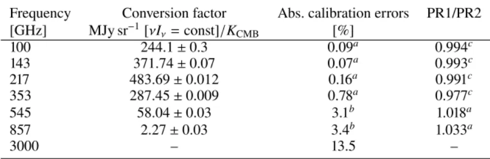
Table 1. Useful numbers used in our analysis.
Frequency Conversion factor Abs. calibration errors PR1/PR2
[GHz] MJy sr−1[νIν= const]/KCMB [%]
100 244.1 ± 0.3 0.09a 0.994c 143 371.74 ± 0.07 0.07a 0.993c 217 483.69 ± 0.012 0.16a 0.991c 353 287.45 ± 0.009 0.78a 0.977c 545 58.04 ± 0.03 3.1b 1.018a 857 2.27 ± 0.03 3.4b 1.033a 3000 – 13.5 –
Notes. The first column gives the unit conversion factors between MJy sr−1[νI
ν = const] and KCMB; the second column gives the error on the absolute calibration; and the third column gives the factors we applied to the Planck CIB measurements to account for a more accurate absolute cali-bration between the two releases of the Planck data (PR1 and PR2).(a)FromPlanck Collaboration VIII(2016a).(b)FromPlanck Collaboration XLVI (2016c).(c)Computed using exactly the same method as that used inPlanck Collaboration VIII(2016a).
Planck Collaboration XXX(2014b), the dust in these new SED
1
templates is warmer at z > 2. We used CAMB1to generate cold
2
dark matter power spectra Plin(k) for given redshifts. For the
3
effective bias, we chose the following parametric form based on
4
redshift evolution of the dark matter halo bias:
5
beff(z)= b0+ b1z+ b2z2. (7)
We also tested alternative parametric forms for the effective bias
6
where the evolution of the bias is slower compared to the above
7
equation. The results are presented in AppendixA.
8
To describe ρSFR, we used the parametric form of the
cos-9
mic star formation rate density proposed byMadau & Dickinson 10 (2014) and given by 11 ρSFR(z)= α (1+ z)β 1+ [(1 + z)/γ]δM yr −1Mpc−3, (8)
where α, β, γ, and δ are free parameters in our CIB model.
12
2.2. CIB–CMB lensing
13
Large-scale distribution of the matter in the Universe
gravitation-14
ally deflects the cosmic microwave background (CMB) photons
15
which are propagating freely from the last scattering surface.
16
This gravitational lensing leaves imprints on the temperature and
17
polarisation anisotropies. These imprints can be used to
recon-18
struct a map of the lensing potential along the line of sight
19
(Okamoto & Hu 2003). Dark matter halos located between us
20
and the last scattering surface are the primary sources for this
21
CMB lensing potential (Lewis & Challinor 2006) and it has been
22
shown (e.g.Song et al. 2003) that a strong correlation between
23
CIB anisotropies and a lensing derived projected mass map is
24
expected.
25
We calculated the cross-correlation between the CIB and
26
CMB lensing potential (Planck Collaboration XVIII 2014a),
27 which is given by 28 Cνφl = Z beff¯j(ν, z) 3 l2ΩmH 2 0 χ∗−χ χ∗χ ! Plin(k= l/χ, z)dχ, (9)
where χ∗ is the comoving distance to the CMB last scattering
29
surface,Ωmis the matter density parameters, and H0is the value
30
of the Hubble parameter today. From Eq. (9), we see that Clν,φis
31
1 http://camb.info/
proportional to beff, whereas CCIBl is proportional to b2eff. There- 32
fore, also using the CIB–CMB lensing potential measurement 33
when fitting the CIB model helps us resolve the degeneracy 34
between the evolution of beffand ρSFRto some extent. 35
2.3. Constraints on the model through data 36
2.3.1. Observational constraints on the power spectra 37
We used the CIB angular power spectra measured by 38
Planck Collaboration XXX (2014b). The measurements were 39
obtained by cleaning the Planck frequency maps from the CMB 40
and galactic dust, and they were further corrected for SZ and 41
spurious CIB contamination induced by the CMB template, as 42
discussed in Planck Collaboration XXX (2014b). We used the 43
measurements at the four highest frequencies (217, 353, 545, 44
and 857 GHz from the HFI instrument). For the 3000 GHz, far- 45
infrared data from IRAS (IRIS,Miville-Deschênes & Lagache 46 2005) were used. As we are using the linear model we fit the 47
data points only for l6 600, which are dominated by the 2-halo 48
term (>90%,Béthermin et al. 2013;Planck Collaboration XXX 49
2014b). 50
CIB–CMB lensing potential cross-correlation values and 51
error bars are available for the six Planck HFI chan- 52
nels (100, 143, 217, 353, 545, and 857 GHz) and are 53
provided in Planck Collaboration XVIII (2014a). These val- 54
ues range from ` = 163 to ` = 1937. As discussed in 55 Planck Collaboration XVIII(2014a), the non-linear term can be 56
neglected in this range of multipoles. 57
We used the νIν = const photometric convention. Thus, 58
the power spectra computed by the model need to be colour- 59
corrected from our CIB SEDs to this convention. Colour cor- 60
rections are 1.076, 1.017, 1.119, 1.097, 1.068, 0.995, and 0.960 61
at 100, 143, 217, 353, 545, 857, and 3000 GHz, respectively 62
(Planck Collaboration XXX 2014b). The CIB power spectra are 63
then corrected as 64
Cmodell,ν,ν0 x ccνx ccν0 = Cl,ν,νmeasured0 . (10)
Calibration uncertainties are not accounted for in the CIB 65
power spectra error bars and are treated differently.Béthermin 66 et al. (2011) introduce a calibration factor fcalν for galaxy 67
number counts. We used a similar approach here. We put 68
Gaussian priors on these calibration factors for different fre- 69
quency channels with an initial value of 1 and the error bars 70
as given in Table1. The CIB measurements from Planck were 71
Table 2. Mean levels of CIB from different instruments at different frequencies with the corresponding colour corrections used to convert them to the Planck and IRAS bandpasses.
Instrument Freq νIν Colour
GHz nWm−2sr−1 correction Herschel/PACS 3000 12.61+8.31−1.74 0.9996 Berta et al.(2011) Herschel/PACS 1875 13.63+3.53−0.85 0.9713 Berta et al.(2011) Herschel/SPIRE 1200 10.1+2.60−2.30 0.9880 Béthermin et al.(2012b) Herschel/SPIRE 857 6.6+1.70−1.60 0.9887 Béthermin et al.(2012b) JCMT/SCUBA2 667 1.64+0.36−0.27 1.0057 Wang et al.(2017) Herschel/SPIRE 600 2.8+0.93−0.81 0.9739 Béthermin et al.(2012b) JCMT/SCUBA2 353 0.46+0.04−0.05 0.9595 Zavala et al.(2017) ALMA 250 > 0.08 – Aravena et al.(2016)
Table 3. Marginalised values of the CIB model parameters provided at a 68% confidence level.
Parameter Marginalised value
α 0.007+0.001−0.001 β 3.590+0.324−0.305 γ 2.453+0.128−0.119 δ 6.578+0.501−0.508 b0 0.830+0.108−0.108 b1 0.742+0.425−0.471 b2 0.318+0.275−0.236 f217cal 1.000+0.002−0.002 f353cal 1.004+0.007−0.007 fcal 545 0.978+0.015−0.014 fcal 857 1.022+0.023−0.023 f3000cal 1.155+0.086−0.089
and PR2 releases, the absolute calibration improved further,
1
and we thus wanted to consider the absolute calibration of
2
the PR2 release for the CIB measurements. Consequently, the
3
CIB × CIB and CIB × CMB lensing power spectra data points
4
were corrected for the absolute calibration difference of the
5
two releases (following the numbers given in Table1), and we
6
used the absolute calibration errors as given for the PR2 release
7
(Planck Collaboration VIII 2016a).
8
2.3.2. External observational constraints
9
To put better constraints on ρSFR and beff parameters, in
addi-10
tion to the CIB × CIB and CIB × CMB lensing angular power
11
spectra, we used some external observational constraints on the
12
star formation rate density at different redshifts, local bias of the
13
dusty galaxies, and mean CIB levels at different frequencies, as
14
detailed below:
15
1. We used the ρSFR measurements at different redshifts that 16
were obtained by measuring the IR luminosity functions 17
from Gruppioni et al. (2013), Magnelli et al. (2013), and 18 Marchetti et al.(2015) (see the discussion in Sect.3.2). This 19
helped us to put better constraints on the parameters. The 20
cosmological parameters used in these studies are different 21
from the ones used here. As mentioned before, we also per- 22
form a Fisher matrix analysis to study the effect of the CIB 23
parameters on cosmology. For this purpose, we needed to 24
convert all the observational ρSFRdata points to actual mea- 25
surements which are cosmology independent. We thus used 26
the observed flux in the range 8–1000 µm (rest frame) per 27
redshift bin per solid angle dBIR
dzdΩ. We perform the conversion 28
as follows: 29 dBIR dzdΩ = d(PIR/4πD2L) dzdΩ (11) = 1 4πD2 L dPIR dVc dVc dzdΩ (12) = 1 4πD2 L ρSFR K DH(1+ z)2D2A E(z) . (13) Here dPIR
dVc is the power emitted in the infrared per unit co- 30
moving volume of space, DL is the luminosity distance, 31
DA is the angular diameter distance, DH is the Hubble 32
distance given by c/H0 (with c and H0 being the speed 33
of light and Hubble’s constant, respectively), and E(z) = 34
p
Ωm(1+ z)3+ Ωk(1+ z)2+ ΩΛ. This equation can be sim- 35
plified further using the relation DL = (1 + z)2DA and 36
becomes 37 dBIR dzdΩ = 1 4π ρSFR K DH(1+ z)2 (1+ z)2E(z). (14)
We also needed to convert the measurements to the same 38
IMF; e.g.Gruppioni et al.(2013),Magnelli et al.(2013), and 39 Marchetti et al.(2015) used the Salpeter IMF, whereas we 40
used the Chabrier IMF. Finally, we used these observed flux 41
values dBIR/dzdΩ in our fitting rather than the ρSFRvalues. 42
This conversion to cosmology-independent variables is par- 43
ticularly important for the Fisher matrix analysis presented 44
in Sect.5, else we would wrongly find that CIB anisotropies 45
can be used to significantly improve the uncertainties on the 46
cosmological parameters. 47
2. Saunders et al.(1992) provide the fixed value for the product 48
of the local bias of infrared galaxies bI and the cosmolog- 49
ical parameter σ8: bIσ8 = 0.69 ± 0.09. We put a constraint 50
of b= 0.83 ± 0.11 on local bias value which has been con- 51
verted using the σ8 measured byPlanck Collaboration XIII 52
(2016b). 53
3. The mean level of the CIB at different frequencies has been 54
deduced from galaxy number counts. The values we used 55
are given in Table 2. Similarly to what is being done for 56
Cl,ν,ν0 (Eq. (10)), the CIB computed by the model needs to 57
be colour-corrected, from our CIB SEDs to the photomet- 58
ric convention of PACS, SPIRE, and SCUBA2. The colour 59
corrections are computed using theBéthermin et al.(2012a) 60
CIB model and the different bandpasses and are given in 61
Table2. 62
4. Finally, we also put physical constraints on ρSFR and beff 63
parameters such that the star formation rate and galaxy bias 64
Fig. 1.Posterior confidence ellipses for the CIB model parameters. All the calibration parameters lie within the 1σ range of their prior values. There is no significant degeneracy between any of the calibration parameters and CIB parameters and hence they are not shown here.
2.3.3. Fitting the data
1
We performed a Markov chain Monte Carlo (MCMC)
2
analysis on the global CIB parameter space. Python
pack-3
age “emcee” (Foreman-Mackey et al. 2013) is used for
4
this purpose. We have a 12-dimensional parameter space:
5 {α, β, γ, δ, b0, b1, b2, f217cal, f cal 353, f cal 545, f cal 857, f cal 3000}. Our global χ 2has 6
a contribution from the CIB × CIB and CIB × CMB lensing
7
angular power spectra measurements, priors on calibration
fac-8
tors, and priors imposed by the external observational constraints
9
mentioned above. We assumed Gaussian uncorrelated error bars
10
for measurement uncertainties. The 1-halo and Poisson terms
11
have very little measurable contribution (less than 10%) at
12
l ≤600, where we are fitting the data points. Similar to the
pro-13
cedure used inPlanck Collaboration XXX(2014b), we added the
14
contribution of these terms derived from the Béthermin et al. 15
(2013) model to our linear model.
16
2.4. Results
17
We present the results from our fit in Table3. We find a good
18
fit for the model and the posterior of all the parameters with a
19
Gaussian prior (local effective bias and calibration factors) are
20
within a 1σ range of the prior values. The 1σ and 2σ confidence
21
regions for the ρSFR and beff parameters are shown in Fig. 1.
22
As expected, we observe strong degeneracies between ρSFRand
23
beff, and also within the ρSFR and beff parameters themselves.
24
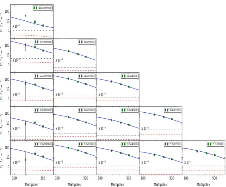
Figures2and3 show the fit for the linear model to the
obser-25
vational data points for all CIB × CIB auto- and cross-power
26
spectra, and CIB × CMB lensing power spectra, respectively. We
27
also show the shot noise and one-halo term for all the frequencies 28
in Fig.2. 29
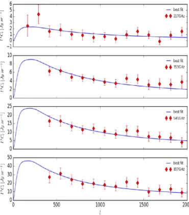
In Fig.3, we show the comparison between our best fit model 30
and the CIB–CMB lensing cross-correlation points. We consider 31
these data points to calculate the best fit of our model. We find a 32
good agreement between the data points and the best fit. 33
3. CIB redshift distribution and star formation 34
history 35
3.1. Redshift distribution of CIB anisotropies and mean level 36
The model we used is based on the SEDs over a range of 37
wavelengths for galaxies which vary with redshift. It is thus inter- 38
esting to study the redshift distribution of the mean level of the 39
CIB as well as the CIB anisotropies which are based on these 40
SEDs. In Fig.4, we show the redshift distribution of the CIB 41
anisotropies at ` = 300 and CIB mean level intensity for dif- 42
ferent frequency bands. Both plots have been normalised, i.e. 43
R
d(νIν)/dz dz= 1 and R dCl/dz dz = 1, so that it is easier to 44
compare the results for different frequencies. 45
It is observed that as we go to lower frequencies, from 3000 46
to 217 GHz, the peak of the CIB anisotropy redshift distribu- 47
tion increases in redshift. This is expected as higher frequencies 48
(lower wavelengths) probe lower redshifts and vice versa (e.g. 49 Lagache et al. 2005;Béthermin et al. 2013). The CIB mean level 50
distribution follows the same trend. A similar pattern is observed 51
for the CIB anisotropy and for the mean level distribution in 52 Béthermin et al.(2013) model. We note, however, that the peak 53
Fig. 2.Measurements of the CIB auto- and cross-power spectra obtained by Planck and IRAS (extracted fromPlanck Collaboration XXX 2014b) and the best fit CIB linear model. Data points on higher ` are not shown as they are not used for fitting. We also show the shot noise (black dash-dotted line) and one-halo term (red dashed line) for all the frequencies.
of CIB anisotropies predicted inBéthermin et al.(2013) at 353
1
and 217 GHz is reached around z= 2.4 and the same is reached
2
at lower redshift (around z= 1.7) for our model.
3
In Fig.5, we compare our redshift distribution on the CIB
4
mean level with the lower limits fromBéthermin et al.(2012c)
5
and Viero et al. (2013) which were derived by stacking the
6
24 µm-selected and mass-selected sources, respectively. It is
7
observed that the CIB mean level from our model is higher than
8
these two lower limits for most of the values. We also
com-9
pare our results with redshift distribution of the CIB derived
10
by Schmidt et al. (2015) using the cross-correlation between
11
the Planck HFI maps and SDSS DR7 quasars. It can be seen
12
that although some of the data points from Schmidt et al. 13
(2015) are consistent with our curve, the measurements tend
14
to be higher than our model at Z > 0.5. A similar trend is
15
followed at other frequencies, and so they are not shown here.
16
Koprowski et al.(2017) assumed a Gaussian distribution for the
17
IR and UV ρSFR and also provided the best fit values for the
18
distribution. Based on this ρSFR form, we calculated the
cor-19
responding mean CIB level distribution using Eqs. (6) and (5)
20
using the SED templates fromBéthermin et al.(2017) (see Fig.5,
21
dashed black curve). It can be seen that their mean CIB level dis- 22
tribution is lower than some lower limits (at z ∼ 1 and z ∼ 3). It 23
is also lower than values from our model between 0.5 < z < 2, 24
and hence in even more tension with the values fromSchmidt 25
et al.(2015). 26
3.2. Star formation history 27
We show the evolution of star formation density with the redshift 28
in Fig.6with the best fit as well as the corresponding 1σ and 2σ 29
confidence regions. We created these confidence regions using 30
the chains from the Monte Carlo sampling of our likelihood. 31
We took random samples from the chains for the star forma- 32
tion density parameters and constructed an array of ρSFR with 33
these samples for all the redshifts. The median of these values 34
at every redshift is then the central value, and we took samples 35
within 68.2% and 95.4% around the central value as 1σ and 2σ 36
regions, respectively. 37
We also show the IR measurements from Gruppioni et al. 38
(2013),Magnelli et al.(2013),Marchetti et al.(2015), andBourne 39 et al.(2017), and UV measurements fromCucciati et al.(2012), 40
Fig. 3.CIB × CMB lensing cross-power spectra. Our best fit model is shown by the blue curves for different frequency channels. Measure-ments (red data points) are fromPlanck Collaboration XVIII(2014a). They have been included in the likelihood to calculate and get better constraints on the CIB linear model.
Fig. 4.Expected CIB mean level and anisotropy redshift distributions are shown in the lower and upper panels, respectively. Both of the distributions have been normalised for easier comparison, and the dif-ferent colours show difdif-ferent frequency bands. The CIB anisotropy distribution is shown for `= 300.
Fig. 5.Expected CIB mean level redshift distribution at 857 GHz com-pared to observational constraints. The lower limits are fromBéthermin et al.(2012c) andViero et al.(2013). They are shown using black and red triangles, respectively. Measurements fromSchmidt et al.(2015) are shown in green. The redshift distribution derived fromKoprowski et al.
(2017) SFRD constraints is shown with the black dashed line.
Bouwens et al.(2012), andReddy & Steidel(2009), in the upper 1
and lower panels, respectively. Our best fit passes through the 2
IR data points considered in the fit. As mentioned in Sect.2.3.2, 3
these data points were obtained using a Salpeter IMF, whereas in 4
our study, we use a Chabrier IMF. Therefore, both the IR and UV 5
data points have been converted to take into account this change. 6
As expected, the UV data points (which have not been cor- 7
rected for dust attenuation) for unobscured star formation density 8
lie below our curves for z < 3 as most of the UV light emit- 9
ted by young and short-lived stars in this regime is reprocessed 10
by dust. Although the IR contribution is still dominant below 11
z < 4, the contribution from the UV becomes significant and 12
roughly equal to IR for z > 4. Hence IR contribution alone is not 13
a good measure of the total star formation rate density at such 14
high redshifts. 15
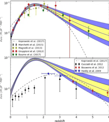
We plot the best fit IR and UV ρSFRcurves fromKoprowski 16 et al.(2017) with dashed black lines in the upper and lower pan- 17
els of Fig.6, respectively. It can be seen that their value of the 18
IR SFRD in the local Universe is higher compared to the other 19
measurements. Also, their IR SFRD drops very quickly at higher 20
redshifts and is basically negligible for z > 4. Their results are 21
clearly discrepant with ours in these two regimes. A similar trend 22
is followed by the UV SFRD which drops quickly and is much 23
smaller than current observational constraints at z ∼ 6. 24
To investigate the discrepancy between our values and the 25 Koprowski et al.(2017) ρSFR, we performed a MCMC fitting for 26
the CIB anisotropy model (as described in Sect.2.3.3) and fitting 27
for the effective bias and the calibration factors, but fixing the 28
SFRD to the best fit ofKoprowski et al.(2017). We found the 29
effective bias at redshifts z > 2.5 to be much higher (>50%) than 30
is observed for the SMGs. This effective bias value is too high 31
compared to what is realistically expected, suggesting that their 32
SFRD is underestimated. 33
Similarly, Fig. 6shows that the Bourne et al.(2017) points 34
at z ' 1 and 2 are a factor >2 and 1.3 below our measurements, 35
Fig. 6.Evolution of star formation density with redshift as constrained by the linear CIB model. The ±1σ and ±2σ confidence region around the median realisation is shown in yellow and blue, respectively. Mea-surements of obscured star formation density from Gruppioni et al.
(2013),Magnelli et al.(2013), andMarchetti et al.(2015), which were used to fit the CIB model, have been added along with the measurements fromBourne et al.(2017) in the upper panel. The Gaussian form of the ρSFRfor the IR obscured star formation rate density used byKoprowski
et al. (2017) has been plotted as the black dashed line in the upper panelwith a corresponding UV part in the lower panel. Unobscured star formation rate density derived from UV fromCucciati et al.(2012),
Bouwens et al.(2012), andReddy & Steidel(2009) are also shown in the lower panel.
those from Gruppioni et al. (2013) would give a lower
mea-1
surement for SFRD and this would affect the measurement of
2
the linear bias. We investigated the consistency of the solution
3
obtained on both ρSFRand beffeither by taking theBourne et al.
4
(2017) data points as priors or by forcing and fixing the SFRD
5
to go through theBourne et al.(2017) data points in our MCMC
6
analysis. We found that the linear bias is severely overestimated
7
compared to similar galaxy populations, for example by a factor
8
>3 at z ' 1.2 compared to the SMG sample ofWilkinson et al. 9
(2017). This shows that the SFRD determined byBourne et al. 10
(2017) at low z seems to be underestimated.
11
4. Host dark matter halos of the CIB
12
4.1. Effective bias of CIB galaxies
13
We also study the evolution of the effective bias and find that it is
14
increasing with redshift, as expected. In Fig.7, we compare our
15
measurements with the clustering measurements of individual
16
galaxies selected using various criteria.
17
At z > 2, our measurements and the clustering of SMGs by
18
Wilkinson et al.(2017) are very similar. SMGs are the most
star-19
forming galaxies at z& 2 (e.g.Blain et al. 2002;Chapman et al. 20
2005), and thus it is not completely surprising to find a
simi-21
lar bias since a large fraction of the SFRD at z > 2 is hosted
22
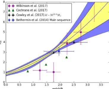
by galaxies forming more than 100 M yr−1 (e.g.Caputi et al. 23 2007; Magnelli et al. 2009; Béthermin et al. 2011; Gruppioni 24 et al. 2013). At z <2,Wilkinson et al.(2017) found a bias close 25
to 1, which is 1σ and 2σ below our model in the 1 < z < 1.5 26
and 1.5 < z < 2 bins, respectively. This might be a statistical 27
fluctuation coming from the small sample in their low-z bins 28
(∼60 objects). In addition, the algorithm they use to associate 29
SMGs with optical counterparts and photometric redshift is only 30
reliable at 83%, which could induce biases in the clustering mea- 31
surements. In the 1.5 < z < 2 bin, if they consider only objects 32
with a solid radio identification of the counterparts, they find a 33
bias of 1.65 ± 1.09, which is compatible at 1σ with our measure- 34
ments, which means that there might be no real tension in these 35
low-z bins. 36
We also compare our bias estimates with selections at other 37
wavelengths.Béthermin et al.(2014) measured the clustering of 38
massive star-forming galaxies at z ∼ 2 selected using the BzK 39
color criterium (Daddi et al. 2004). Our effective bias agrees 40
with this measurement. Viero et al. (2013) show that major- 41
ity of the contribution to the CIB is emitted by massive dusty 42
star-forming galaxies with log(M/M ) 10.0–11.0. We plot the 43
clustering of the mass-selected (M?= 1010.6M ) galaxies mea- 44
sured by Cowley et al.(2018) and find an agreement with our 45
measurements, as expected.Ishikawa et al.(2015) measured the 46
clustering of gzKs-selected galaxies for various depths and found 47
a strong dependance of bias with the depth. Their deep sample 48
(K ≤ 23) has a much smaller bias than the CIB (1.8 vs. 3.1), but 49
the shallowest sample (K ≤ 21) has a stronger bias (4.16). The 50
CIB measurements are indeed dominated by the galaxies, which 51
contribute the most to the star formation budget, while cluster- 52
ing measurements of galaxy populations are dominated by the 53
most numerous objects, which are usually the numerous low- 54
mass objects residing in low-mass halos (Mhalo< 1012M ) with 55
a lower clustering. It is thus expected that the deepest K-band 56
sample with masses and SFRs well below the knees of the mass 57
and SFR functions have a lower bias than the CIB. In a similar 58
way, the bias of Hα-selected galaxies, which are mainly low-SFR 59
and low-mass galaxies, measured byCochrane et al.(2017) (1.12, 60
1.78, 2.52), is significantly lower than our model (1.64, 2.62, 61
4.06) at redshifts 0.8, 1.47, 2.23 respectively. 62
4.2. What does the effective bias mean? 63
Throughout the paper, we have used the effective bias term (beff) 64
and it should be noted that effective bias might not be equal to 65
the mean bias of halos hosting the dusty galaxies (b(M, z)). As 66
shown in Appendix C ofPlanck Collaboration XXX(2014b), the 67
effective bias is the mean bias of halos hosting the dusty galaxies 68
weighted by their differential contribution to the emissivities and 69
is given by the following equation: 70
beff= R d j dM(ν, z)b(M, z)dM R d j dMdM . (15)
In this equation, dMd j is the differential contribution of a range 71
of halo mass to the emissivity. Since the emissivity is directly 72
proportional to ρSFR, we can rewrite this equation as 73
beff= P vol SFR × b(M, z) P vol SFR , (16)
where we sum over all the halos and their host galaxies in a 74
Fig. 7. Evolution of the effective bias with redshift derived from the CIB compared to the observational values obtained on selected pop-ulations of galaxies:Béthermin et al. (2014),Cochrane et al.(2017),
Cowley et al. (2018), and Wilkinson et al. (2017) using a sample of BzK-selected galaxies, Hα-selected galaxies, mass-selected galaxies, and SMGs, respectively.
halo mass and redshift, is calculated with the formula which
1
has been calibrated using the numerical simulations fromTinker 2 et al.(2010), 3 b(ν)= 1 − A ν a νa+ δa c + Bνb+ Cνc, (17)
where ν = δc/σM characterises the peak heights of the
den-4
sity field as function of mass and redshift; δc is the linear
5
critical density at a given redshift for a given cosmology; and
6
σM is the linear matter variance in a top hat filter of width
7
R = (3M/4π ¯ρ0)1/3 with M and ¯ρ0 being the mass and mean
8
density for a given halo, respectively. Details of these
calcula-9
tions have been given in Appendix A of Coupon et al.(2012).
10
A, a, B, b, C, and c are functions of ∆ which is the overdensity for
11
a given halo defined as the mean interior density for the halo
rel-12
ative to the background. These functions are provided in Table 2
13
inTinker et al.(2010). As often used, we took a virial value of
14
∆ ≈ 200. From Eq. (15), we can see that if halos in a given mass
15
range contribute more or less to the emissivity compared to halos
16
of a different mass range, there will be a slight offset between beff
17
and b(M, z).
18
It is interesting to quantify this offset, particularly in the
con-19
text of the measurement of the mass of the typical host dark
20
matter halos which contribute to the CIB, and hence to the
21
obscured star formation. This is the purpose of the next section.
22
As a first approximation, we can estimate the mean host halo
23
mass at a given redshift by equating beffand b(M, z). At z= 2,
24
we find that the mass of the dark matter halos which contribute
25
the most to the CIB calculated this way is log10M = 12.93+0.084−0.081,
26
where 0.084 and 0.081 are the 1σ upper and lower limits,
27
respectively.
28
4.3. Host dark matter halo mass of the dusty star formation
29
As is shown in the previous section, beff might not be exactly
30
equal to the mean bias of halos hosting the dusty galaxies
31
(b(M, z)). To understand how this effective bias relates to the
32
Fig. 8.Normalised cumulative SFR density and LIR density as a func-tion of host dark matter halo mass for galaxies in SIDES simulafunc-tion are shown in red and green, respectively. We also show the variation of these quantities when they are weighted with the corresponding bias value for the galaxies in blue and black, respectively. The black vertical line represents the mass of the dark matter halo mass calculated con-verting the beffobtained using the LIR instead of the SFR into the halo mass using Eqs. (17) and (16) (replacing SFR by LIR). The horizontal line represents the 50% cumulative level. This plot has been made for the galaxies in the range 2.0 < z < 2.2.
bias of the halos contributing the most to the star formation 33
budget, we used the Simulated Infrared Dusty Extragalactic Sky 34
(SIDES) simulation (Béthermin et al. 2017), where the impact of 35
clustering and angular resolution for far-infrared and millimetre 36
continuum observations has been taken into account. 37
The SIDES simulation provides the star formation rate for 38
galaxies corresponding to a given halo mass Mhaloat a given red- 39
shift z. In Fig.8we plot the cumulative star formation rate as a 40
function of halo masses for galaxies with 2.0 < z < 2.2. We can 41
see from the red curve in Fig.8how the cumulative SFR den- 42
sity grows with the halo masses in SIDES. We define the mass 43
at which the above curve reaches 50% of the total cumulative 44
star formation as the dark matter halo mass hosting the dusty 45
galaxies. 46
We calculated the bias b(M, z) corresponding to each halo 47
at a given redshift in SIDES using Eq. (17). The blue curve 48
in Fig.8, shows how the normalised cumulative SFR × b(M, z) 49
grows with the halo mass. It is seen that 50% of the total SFR 50
or SFR×b is reached around a halo mass of 1012M , but not at 51
the exact same halo mass. Since the bias is higher for massive 52
halos hosting more massive and star-forming galaxies, we reach 53
these 50% for SFR × b at a mass 0.06 dex higher than for just 54
SFR. The effective bias of the CIB, thus corresponds to a bias 55
slightly higher than the bias of the pivot halo mass at which we 56
have 50% of the SFRD. This value of 0.06 dex, however, is still 57
not the offset we should apply to the mass log10M= 12.93+0.084−0.081 58
of the host dark matter halo obtained using beff. 59
The CIB traces only the obscured star formation, but at low 60
stellar mass (and thus halo mass), a significant fraction of the 61
UV from the star formation escapes the galaxies. We used the 62
method ofBernhard et al.(2014) based on the empirical relation 63
between stellar mass and dust attenuation ofHeinis et al.(2014) 64
to predict the SFRIR, i.e. the obscured star formation, from which 65
the simulation. In Fig.8, the green and black curves represent the
1
cumulative contribution of the LIRand the LIR× b, respectively.
2
This latest quantity (LIR× b) is the closest to what we actually
3
measure with the CIB. The halo mass at which 50% of the total
4
quantity is reached for slightly higher halo mass (0.05 dex) than
5
that found for SFR × b because obscured star formation is slightly
6
biased toward massive galaxies (and thus halos). For the dark
7
matter halos between 2 < z < 2.2, we observe a difference of
8
around 0.11 dex between halo masses found using only the SFR
9
and the bias weighted LIR (LIR× b). Using Eq. (16), we can
cal-10
culate the beffcorresponding to these LIR values where we just
11
replace the SFR term in the equation with the LIR obtained here.
12
Using the procedure followed in Sect.4.2, we convert this beffto
13
the corresponding halo mass using Eq. (17). The black vertical
14
line in Fig.8represents this mass of the dark matter halo. Finally,
15
the difference between this mass and halo mass found using only
16
the SFR, which is 0.10 dex, is the actual offset we are looking for
17
at this redshift bin.
18
Following the procedure mentioned above, we calculate this
19
mass offset for all the redshift bins. This offset is shown in Fig.9.
20
The dashed blue line in the figure shows the mean value of the
21
offset over all the bins which is around 0.16 dex. It is clear from
22
the figure that this offset is not constant at all redshifts. After
23
applying this mean correction to the halo masses at all the
red-24
shifts, we also propagate the uncertainty on this offset to the
25
error bars on the mass measurements. We find that the mass of
26
the dark matter halos which contribute the most to the CIB at
27
z= 2 comes out to be log10M = 12.77+0.128−0.125, where 0.128 and
28
0.125 are the 1σ upper and lower limits, respectively
(consid-29
ering additional uncertainty on mass offset), compared to the
30
previous value of log10M = 12.93+0.084−0.081.
31
We show in Fig.10the variation of the host halo mass as a
32
function of redshift for z ≤ 4. Contours represent the 1σ and 2σ
33
confidence regions. We obtain an almost constant dark matter
34
halo mass (≈ 1012.7M
) contributing to the CIB from 1 < z < 4,
35
and then it starts decreasing from z < 1. Host halos grow over
36
time and the dashed lines show this growth of halos with
red-37
shift, as computed byFakhouri et al. (2010). We see that most
38
of the star formation at z > 2.5 occurred in the progenitors of
39
clusters (Mh(z = 0) > 1013.5M ). Then at the lower redshifts
40
from 0.3 < z < 2.5, most of the stars were formed in groups
41
(1012.5 < M
h(z = 0) < 1013.5M ) and later on, finally, inside
42
the Milky Way-like halos (1012 < Mh(z= 0) < 1012.5M ) for
43
z< 0.3. Although a bit high, these results are compatible with
44
the results obtained byBéthermin et al.(2013).
45
5. Effect of cosmology on CIB
46
5.1. Method
47
All the previous studies on the CIB were performed assuming a
48
fixed fiducial cosmology. We can see the role of the
cosmologi-49
cal parameters for the CIB through Eq. (5) where the CIB power
50
spectrum depends upon the dark matter power spectrum,
Hub-51
ble’s constant, cosmological energy density parameters (through
52
distance measures), etc. It was thus interesting to study the effect
53
of cosmology on the CIB, i.e. whether changing the cosmology
54
makes a significant impact on the CIB parameters. In order to
55
study this effect, we performed a Fisher matrix analysis over all
56
12 CIB parameters and 6 cosmological parameters.
57
For an N-variate multivariate normal distribution X ∼
58
N(µ(θ),Σ(θ)), the (m, n) entry of the Fisher matrix is given as
59
Fig. 9. Difference between the dark halo mass estimated as the halo mass where 50% cumulative SFR (Mh SFR 50%) is achieved and the halo mass calculated by converting the beff, which is obtained using the LIR (replacing SFR with LIR in Eq. (16)) to the corresponding halo mass using Eq. (17) (MhLIR weighted). This difference has been calcu-lated and is shown here for all the redshift bins. The dashed line shows the mean of these values: around 0.16 dex. This is the offset applied to the halo mass derived from beff to obtain the mean mass of dark matter halos contributing to CIB.
Fig. 10.Mass of the dark matter halos hosting the galaxies contributing to the CIB as a function of redshift. The black dashed lines show the growth of the dark matter halo mass with redshift. The red dashed line shows the mass that would be obtained directly equating beffand b(M, z) (see Sect.4.2). 60 Im,n=∂θ∂µ mΣ −1∂µ T ∂θn + 1 2tr Σ −1 ∂Σ ∂θmΣ −1∂Σ ∂θm ! , (18)
where ()Tdenotes the transpose of a matrix and tr() denotes the 61
trace of a square matrix; θ = [θ1, . . . , θK] is a K-dimensional 62
vector of parameters being considered; µ(θ)= [µ1(θ), . . . , µN(θ)] 63
are the mean values of the N random variables for which the 64
uncertainties on their measurements are available; Σ(θ) is the 65
covariance matrix for all the variables µ(θ); and 66
∂µ ∂θm ="∂µ1 ∂θm , . . . ,∂µN ∂θm # (19)
is a vector of the partial derivatives of the N variables for a given
1
parameter θm. In our case,Σ(θ) = constant, i.e. the covariance
2
matrix is independent of the parameters and hence the second
3
term in Eq. (18) vanishes as ∂Σ ∂θm = 0, and therefore 4 Im,n=∂θ∂µ m Σ−1∂µT ∂θn . (20)
In our case, the parameters being considered are θ =
5
[α, β, γ, δ, b0, b1, b2, fνcal, H0, Ωbh2, Ωch2, τ, ns, As]. In the
follow-6
ing sections, we explain the construction of the ∂µ ∂θ and Σ 7 matrices. 8 5.2. ∂µ∂θ matrix construction 9
Figure11shows the different components of the ∂µ∂θ matrix. To
10
construct this matrix, we have to calculate the partial derivatives
11
of all the variables with respect to all the CIB and
cosmologi-12
cal parameters. For every parameter θm, the partial derivative is
13 calculated as 14 ∂µ ∂θm = µ(Θ, θm+ δθm) − µ(Θ, θm−δθm) 2δθm , (21)
where while calculating the partial derivative for a parameter θm,
15
all the other parameters represented here byΘ are kept constant
16
at their best fit value. As we are performing the Fisher
analy-17
sis to see the relative effect of cosmological parameters on CIB,
18
we assume a fiducial cosmology and treat all the cosmological
19
parameters as priors. We maintain the value of δθ small enough
20
to ensure that we are within the Gaussian region for a given
21
parameter.
22
Component I in the upper left part of the matrix contains
23
the observational constraints mentioned in Sect.2.3.1, i.e. CIB
24
auto- and cross-power spectra, priors on calibration factors fcal ν ,
25
and CIB–CMB lensing cross-correlation points for all the
fre-26
quencies. Component II in the same upper left part of the
27
figure contains the external observational constraints mentioned
28
in Sect.2.3.2, which are the ρSFR observations, prior on local
29
bias, and mean level of CIB at different frequencies. It should
30
be noted that all the ρSFRvalues have been calculated by
differ-31
ent groups using different cosmologies. In order to perform the
32
Fisher analysis, we needed to make them cosmology
indepen-33
dent and therefore we converted them to observed flux values
34
using Eq. (14) assuming a single fiducial Planck 2015 cosmology
35
for all the points. Components III and IV in the lower left part
36
of Fig.11calculate the effect of the six cosmological parameters
37
on the CIB variables (observational constraints in component III
38
and external observational constraints in component IV).
39
Calculations in some of the cases are simplified as certain
40
variables are dependent on only one of the parameters, for
exam-41
ple the Gaussian prior on the calibration factor for a given
42
frequency fcal
ν is independent of all the parameters except itself,
43
and its partial derivative with respect to itself is one. Therefore,
44
the column vector corresponding to this variable in the matrix
45
would simply be {0, 0, . . . , 1, 0, . . . , 0}.
46
Component V in the upper right part of the matrix calculates
47
the effect of CIB parameters on six cosmological parameters.
48
As mentioned above, we treat cosmological parameters as
pri-49
ors, hence they are independent of the CIB parameters, and their
50
partial derivatives with respect to CIB parameters is zero.
There-51
fore, this part of a matrix is an array of the size 12 × 6 with all
52
Fig. 11.Details of the matrix ∂µ ∂θm
used in the Fisher matrix analysis.
Fig. 12.Details of the matrixΣ used in the Fisher matrix analysis.
the elements being zero. Similarly, component VI of the matrix 53
is a diagonal matrix with all the diagonal entries being one and 54
all the off-diagonal elements being zero. 55
5.3.Σ matrix construction 56
TheΣ matrix is the covariance matrix and it contains the infor- 57
mation of the error bars for the variables used in the∂µ
∂θ matrix. 58
As mentioned in Sect.2.3.3, we assume Gaussian uncorrelated 59
error bars for the data points and this makes it relatively easy 60
to construct this matrix. Its elements are shown in Fig.12. The 61
upper left panel of the figure contains the covariance matrix 62
from the CIB variables, which contains the observational and 63
the external observational constraints. As there is no correlation 64
between different CIB variables, the upper left panel is just a 65
diagonal matrix with component I containing the square of the 66
error bars for every variable. The off-diagonal components II 67
and III are both zero. We treat the cosmological parameters as 68
priors. Cosmological parameters are very well constrained by 69
Planck (see Planck Collaboration XIII 2016b) and the Monte 70
Carlo sampling chains for their likelihood is provided on the 71
Planck Legacy Archive2. We used these chains to calculate the
72
covariance matrix between the six cosmological parameters. 73
This matrix goes in component VI of Fig.12. Components IV 74
and V are matrices with all the elements being zero. 75
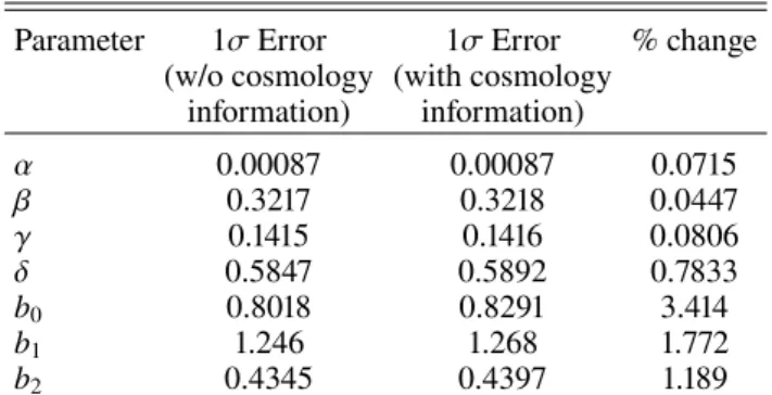
Table 4. Fisher analysis results for the CIB parameters.
Parameter 1σ Error 1σ Error % change
(w/o cosmology (with cosmology information) information) α 0.00087 0.00087 0.0715 β 0.3217 0.3218 0.0447 γ 0.1415 0.1416 0.0806 δ 0.5847 0.5892 0.7833 b0 0.8018 0.8291 3.414 b1 1.246 1.268 1.772 b2 0.4345 0.4397 1.189
Notes. This table gives the error on the CIB model parameters and fcal ν taking into account or not the errors on the cosmological parameters.
Once we have∂µ∂θ andΣ matrices, it is straightforward to
cal-1
culate the entries of the Fisher matrix with Eq. (20); in our case,
2
has the dimensions of (18,18).
3
5.4. Results
4
We show the results from our Fisher matrix analysis in Table4.
5
The error bars on the CIB parameters change very little when
6
we add the effect of varying the cosmological parameters. The
7
change in the error bars on the parameters varies from 0.04% to
8
3.4% which is within the uncertainties on the CIB parameters.
9
Therefore, we conclude that the cosmological parameters
deter-10
mined at the current level of precision have a negligible impact
11
on the CIB model.
12
6. Conclusion
13
We have developed a linear CIB model and used conjointly
14
the CIB anisotropies and CIB × CMB lensing cross-correlations
15
measured at large scale by Planck to determine the SFRD up
16
to z = 6 and the evolution of the effective bias. Our paper
17
improved upon the analysis of the linear CIB model performed
18
by Planck Collaboration XXX (2014b). We used a functional
19
form for the SFRD (Madau & Dickinson 2014) and a polynomial
20
functional form for the effective bias evolution with redshift.
21
We use effective SEDs derived from the latest observations and
22
modelling (Béthermin et al. 2015, 2017). The inclusion of the
23
CIB–CMB lensing cross-correlation in our fitting helps us to
24
partially break the degeneracy between the effective bias and the
25
SFRD parameters. In order to get better constraints on the SFRD
26
parameters, we also used external observational constraints on
27
the SFRD at different redshifts from different surveys which are
28
converted to observed flux values to account for the different
cos-29
mologies used in the analysis. We also used the mean level of the
30
CIB measured at different frequencies to get a better constraint
31
on the CIB model parameters. Gaussian priors have been put on
32
the local value of the effective bias along with the calibration
33
factors for different frequencies where the improved values of
34
the uncertainties on the calibration factors from Planck PR2 data
35
release compared to the PR1 data have been taken into account.
36
With these improved constraints on the CIB model
param-37
eters, we derived the SFRD of dusty galaxies up to z= 6. We
38
showed that UV SFRD measurements are consistently lower than
39
our IR SFRD measurement for z < 4 and become compatible
40
(at 1σ) with the IR SFRD at z= 5. The effective bias increases
41
steeply with redshift and is compatible with a number of other
42
measurements, and in particular with the bias obtained from the
43
mass-selected M? = 1010.6M sample ofCowley et al.(2018), 44
as expected from the mass distribution of the CIB (Viero et al. 45 2013). The possible deviation in the redshift bin 1.5 < z < 2 with 46
the SMG sample ofWilkinson et al.(2017) might be a statisti- 47
cal fluctuation arising from the small sample size in this redshift 48
bin. Consistency checks performed on the ρSFRand effective bias 49
revealed that the IR SFRD fromBourne et al.(2017) at z ' 1 and 50 Koprowski et al.(2017) at z > 3.5 are underestimated. We found 51
that the redshift distribution of the CIB mean was consistently 52
above the published lower limits and that it peaks at z ∼ 1.7 at 53
353 and 217 GHz. 54
Having measured the effective bias value, we have estimated 55
the typical host dark matter halo mass of galaxies contributing 56
to the CIB. As the effective bias of the galaxies we measure is 57
weighted by their SFR (and even more specifically by their LIR), 58
the value of the host dark matter halo mass obtained using the 59
effective bias value has to be corrected. We have used the SIDES 60
simulations fromBéthermin et al.(2017) to quantify the ampli- 61
tude of the correction, which is found to be 0.1 dex. Using this 62
offset, we find that the typical mass of the host halos contributing 63
to the CIB is log10M= 12.77+0.128−0.125at z= 2, which is slightly on 64
the high side of the range 1012.1±0.5M to 1012.6±0.1M found by 65 Viero et al.(2013) andPlanck Collaboration XXX(2014b) but in 66
very good agreement withChen et al.(2016) for faint SMGs of 67
log10M = 12.7+0.1−0.2. 68
Finally, we have quantified for the first time the effect of 69
the cosmology on the CIB parameters. All the previous stud- 70
ies on the CIB had been performed using a fiducial background 71
cosmology. We performed a Fisher matrix analysis to study the 72
effect of changing the cosmology on the CIB and found that it is 73
negligible compared to the existing measurement uncertainties 74
on the CIB parameters. 75
Acknowledgements.We acknowledge financial support from the “Programme 76
National de Cosmologie and Galaxies” (PNCG) funded by CNRS/INSU-IN2P3- 77
INP, CEA, and CNES, France; from the ANR under the contract ANR-15-CE31- 78
0017; and from the OCEVU Labex (ANR-11-LABX-0060) and the A*MIDEX 79
project (ANR-11-IDEX-0001-02) funded by the “Investissements d’Avenir” 80
French government programme managed by the ANR. Abhishek Maniyar 81
warmly thanks Sylvain De la Torre and Carlo Schimd for the enlightening 82
discussions on the Fisher matrix analysis. 83
References 84
Adelberger, K. L., Steidel, C. C., Pettini, M., et al. 2005,ApJ, 619, 697 85
Amblard, A., Cooray, A., Serra, P., et al. 2011,Nature, 470, 510 86
Aravena, M., Decarli, R., Walter, F., et al. 2016,ApJ, 833, 68 87
Bernhard, E., Béthermin, M., Sargent, M., et al. 2014,MNRAS, 442, 509 88
Berta, S., Magnelli, B., Nordon, R., et al. 2011,A&A, 532, A49 89
Béthermin, M., Dole, H., Lagache, G., Le Borgne, D., & Penin, A. 2011,A&A, 90
529, A4 91
Béthermin, M., Daddi, E., Magdis, G., et al. 2012a,ApJ, 757, L23 92
Béthermin, M., Le Floc’h, E., Ilbert, O., et al. 2012b,A&A, 542, A58 93
Béthermin, M., Le Floc’h, E., Ilbert, O., et al. 2012c,A&A, 542, A58 94
Béthermin, M., Wang, L., Doré, O., et al. 2013,A&A, 557, A66 95
Béthermin, M., Kilbinger, M., Daddi, E., et al. 2014,A&A, 567, A103 96
Béthermin, M., Daddi, E., Magdis, G., et al. 2015,A&A, 573, A113 97
Bethermin, M., Wu, H.-Y., Lagache, G., et al. 2017,A&A, 607, A89 98
Blain, A. W., Smail, I., Ivison, R. J., Kneib, J.-P., & Frayer, D. T. 2002, 99
Phys. Rep., 369, 111 100
Bourne, N., Dunlop, J. S., Merlin, E., et al. 2017,MNRAS, 467, 1360 101
Bouwens, R. J., Illingworth, G. D., Oesch, P. A., et al. 2012,ApJ, 754, 83 102
Caputi, K. I., Lagache, G., Yan, L., et al. 2007,ApJ, 660, 97 103
Casey, C. M., Narayanan, D., & Cooray, A. 2014,Phys. Rep., 541, 45 104
Chabrier, G. 2003,PASP, 115, 763 105
Chapman, S. C., Blain, A. W., Smail, I., & Ivison, R. J. 2005,ApJ, 622, 772 106
Cochrane, R. K., Best, P. N., Sobral, D., et al. 2017,MNRAS, 469, 2913
1
Cooray, A., Amblard, A., Wang, L., et al. 2010,A&A, 518, L22
2
Coupon, J., Kilbinger, M., McCracken, H. J., et al. 2012,A&A, 542, A5
3
Cowley, W., Caputi, K., Deshmukh, S., et al. 2018,ApJ, 853, 69
4
Cowley, W. I., Lacey, C. G., Baugh, C. M., & Cole, S. 2016,MNRAS, 461,
5
1621
6
Cucciati, O., Tresse, L., Ilbert, O., et al. 2012,A&A, 539, A31
7
Daddi, E., Cimatti, A., Renzini, A., et al. 2004,ApJ, 617, 746
8
Dole, H., Lagache, G., Puget, J.-L., et al. 2006,A&A, 451, 417
9
Fakhouri, O., Ma, C.-P., & Boylan-Kolchin, M. 2010,MNRAS, 406, 2267
10
Foreman-Mackey, D., Hogg, D. W., Lang, D., & Goodman, J. 2013,PASP, 125,
11
306
12
Gispert, R., Lagache, G., & Puget, J. L. 2000,A&A, 360, 1
13
Gruppioni, C., Pozzi, F., Rodighiero, G., et al. 2013,MNRAS, 436, 2875
14
Heinis, S., Buat, V., Béthermin, M., et al. 2014,MNRAS, 437, 1268
15
Hickox, R. C., Wardlow, J. L., Smail, I., et al. 2012,MNRAS, 421, 284
16
Ishikawa, S., Kashikawa, N., Toshikawa, J., & Onoue, M. 2015,MNRAS, 454,
17 205 18 Kaiser, N. 1986,MNRAS, 222, 323 19 Kennicutt, Jr. R. C. 1998,ARA&A, 36, 189 20
Knox, L., Cooray, A., Eisenstein, D., & Haiman, Z. 2001,ApJ, 550, 7
21
Koprowski, M. P., Dunlop, J. S., Michałowski, M. J., et al. 2017,MNRAS, 471,
22
4155
23
Lagache, G., Puget, J.-L., & Dole, H. 2005,ARA&A, 43, 727
24
Lagache, G., Bavouzet, N., Fernandez-Conde, N., et al. 2007,ApJ, 665, L89
25
Lewis, A., & Challinor, A. 2006,Phys. Rep., 429, 1
26
Madau, P., & Dickinson, M. 2014,ARA&A, 52, 415
27
Maddox, S. J., Dunne, L., Rigby, E., et al. 2010,A&A, 518, L11
28
Magnelli, B., Elbaz, D., Chary, R. R., et al. 2009,A&A, 496, 57 29
Magnelli, B., Popesso, P., Berta, S., et al. 2013,A&A, 553, A132 30
Marchetti, L., Vaccari, M., & Franceschini, A. 2015, IAU General Assembly, 31
2257521 32
Miville-Deschênes, M.-A., & Lagache, G. 2005,ApJS, 157, 302 33
Mo, H. J., & White, S. D. M. 1996,MNRAS, 282, 347 34
Nguyen, H. T., Schulz, B., Levenson, L., et al. 2010,A&A, 518, L5 35
Okamoto, T., & Hu, W. 2003,Phys. Rev. D, 67, 083002 36
Planck Collaboration XVIII. 2011,A&A, 536, A18 37
Planck Collaboration XVIII. 2014a,A&A, 571, A18 38
Planck Collaboration XXX. 2014b,A&A, 571, A30 39
Planck Collaboration VIII. 2016a,A&A, 594, A8 40
Planck Collaboration XIII. 2016b,A&A, 594, A13 41
Planck Collaboration XLVI. 2016c,A&A, 596, A107 42
Reddy, N. A., & Steidel, C. C. 2009,ApJ, 692, 778 43
Saunders, W., Rowan-Robinson, M., & Lawrence, A. 1992, MNRAS, 258, 44
134 45
Schmidt, S. J., Ménard, B., Scranton, R., et al. 2015,MNRAS, 446, 2696 46
Song, Y.-S., Cooray, A., Knox, L., & Zaldarriaga, M. 2003,ApJ, 590, 664 47
Tinker, J. L., Robertson, B. E., Kravtsov, A. V., et al. 2010,ApJ, 724, 878 48
Viero, M. P., Moncelsi, L., Quadri, R. F., et al. 2013,ApJ, 779, 32 49
Wang, W.-H., Lin, W.-C., Lim, C.-F., et al. 2017,ApJ, 850, 37 50
Wechsler, R. H., Gross, M. A. K., Primack, J. R., Blumenthal, G. R., & Dekel, 51
A. 1998,ApJ, 506, 19 52
Weiß, A., Kovács, A., Coppin, K., et al. 2009,ApJ, 707, 1201 53
Wilkinson, A., Almaini, O., Chen, C.-C., et al. 2017,MNRAS, 464, 1380 54
Williams, C. C., Giavalisco, M., Porciani, C., et al. 2011,ApJ, 733, 92 55