Anisotropies in the cosmic microwave background: Theoretical foundations

International Journal o f Theoretical Physics, Vol. 36, No. I1, 1997

Anisotropies in the Cosmic Microwave Background:

Theoretical Foundations

R u t h D u r r e r t

Received June 25, 1997

The analysis of anisotropies in the cosmic microwave background (CMB) has become an extremely valuable tool for cosmology. There is even hope that planned CMB anisotropy experiments may revolutionize cosmology. Together with determinations of the CMB spectrum, they represent the first precise cosmological measurements. The value of CMB anisotropies lies in large part in the simplicity of the theoretical analysis. Fluctuations in the CMB can be determined almost fully within linear cosmological perturbation theory and are not severely influenced by complicated nonlinear physics. In this contribution the different physical processes causing or influencing anisotropies in the CMB are discussed: the geometry perturbations at and after last scattering, the acoustic oscillations in the baryon-photon plasma prior to recombination, and the diffusion damping during the process of recombination. The perturbations due to the fluctuating gravitational field, the so-called Sachs-Wolfe contribution, is described in a very general form using the Weyl tensor of the perturbed geometry.

1. I N T R O D U C T I O N

T h e f o r m a t i o n o f c o s m o l o g i c a l structure in the universe, i n h o m o g e n e i t i e s in the m a t t e r d i s t r i b u t i o n such as quasars at redshifts up to z - - 5, g a l a x i e s , clusters, s u p e r c l u s t e r s , voids, and walls, is an o u t s t a n d i n g , b a s i c a l l y u n s o l v e d p r o b l e m w i t h i n the s t a n d a r d m o d e l o f c o s m o l o g y . W e a s s u m e that the o b s e r v e d i n h o m o g e n e i t i e s are f o r m e d f r o m s m a l l initial fluctuations by g r a v i - tational clustering.

A t first sight it s e e m s o b v i o u s that s m a l l d e n s i t y e n h a n c e m e n t s can g r o w sufficiently r a p i d l y by g r a v i t a t i o n a l instability. But g l o b a l e x p a n s i o n o f the universe and r a d i a t i o n p r e s s u r e c o u n t e r a c t gravity, so that, e.g., in the case o f a r a d i a t i o n - d o m i n a t e d , e x p a n d i n g u n i v e r s e no d e n s i t y i n h o m o g e n e i t i e s can g r o w significantly. E v e n in a universe d o m i n a t e d by p r e s s u r e l e s s matter, i D~partement de Physique Th~orique, Universit~ de Gen~ve, CH-1211 Geneva 4, Switzerland.

2469

cosmic dust, growth of density perturbations is strongly reduced by the expansion of the universe.

Furthermore, we know that the universe was extremely homogeneous and isotropic at early times. This follows from the isotropy of the 3 K cosmic microwave background (CMB), which represents a relic of the plasma of baryons, electrons, and radiation at times before protons and electrons com- bined to neutral hydrogen. After a long series of upper bounds, measurements with the DMR instrument aboard the COsmic Background Explorer satellite (COBE) have finally established anisotropies in this radiation (Smoot et al.,

1992; Wright et al., 1992) at the level of

(.(T(n) - F(n'))2_ t( ~ lO-'~ ~ angular scales 7~ -- 0 -< 90~

n-n' =cos0)

Such an angle-independent spectrum of fluctuations on large angular scales is called a Harrison-Zel'dovich spectrum (Harrison, 1970; Zel'dovich, 1972). It is defined by yielding constant mass fluctuations on horizon scales at all time, i.e., if ln(t) denotes the expansion scale at time t,

((~d4/M) 2 (h = ln)) = const, independent of time

The COBE result, the observed spectrum and amplitude of fluctuations, strongly support the gravitational instability picture.

There exist two main classes of models which predict a Harrison- Zel'dovich spectrum of primordial fluctuations: In the first class, quantum fluctuations expand to super Hubble scales during a period of inflationary expansion in the very early universe and 'freeze in' as classical fluctuations in energy density and geometry (Mukhanov et al., 1991). In the second class, a phase transition in the early universe at a temperature of about 1016 GeV leads to topological defects which induce perturbations in the geometry and in the matter content of the universe (Kibble, 1980). Both classes of models are in basic agreement with the COBE findings, but differ in their prediction of anisotropies on smaller angular scales.

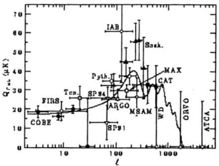
On smaller angular scales the observational situation is somewhat con- fusing and contradictory (Smoot and Scott, 1994; Hu et al., 1997), but many anisotropies have been measured with a maximum of about A T / T ~ (3 - 2) x 10 -5 at angular scale 0 ~ (1 _+ 0.5) ~ There is justified hope that the experiments planned and underway will improve this situation within the next few years. Figure 1, presents the experimental situation as of'spring 1996. In this paper we outline a formal derivation of general formulas which can be used to calculate the CMB anisotropies in a given cosmological model. Since we have the chance to address a community of relativists, we make full use of the relativistic formulation of the problem. In Section 2 we derive,

Anisotropies in CMB: Theoretical Foundations

2471 TO 8 U .50 ~ 4 U ~O 1 0 O I i I I I I I I I I J = -- p.,utl

--

T"~-I 8 P , ~

1 o ' ' ' ' ' " l a I I I i | i i I i I i i l I : OO OOO

l

, 2

Fig. 1. The corresponding quadrupole amplitude Qn~ versus the corresponding spherical har- monic index e. The amplitude Qn~t(s corresponds roughly to the temperature fluctuation on

the angular scale 0 - -rr/e. The solid line indicates the predictions from a standard cold dark

matter model. Figure taken from Smoot and Scott (1994).

Liouville's equation for massless particles in a perturbed Friedmann universe. In Section 3 we discuss the effects of nonrelativistic Compton scattering prior to decoupling. This fixes the initial conditions for the solution to the Liouville equation and leads to a simple approximation of the effect of collisional damping. In the next section we illustrate our results with a few simple examples. Finally, we summarize our conclusions.

N o t a t i o n We denote conformal time by t. Greek indices run from 0 to 3, Latin indices run from 1 to 3. The metric signature is chosen ( - + + +). The Friedmann metric is thus given by ds 2 = a 2 ( t ) ( - d t 2 + ~odxidxJ), where "y denotes the metric of a 3-space with constant curvature K. Three-dimensional vectors are denoted by boldface symbols. We set h = c = kBoltzm~n, = 1 throughout.

2. T H E L I O U V I L L E E Q U A T I O N F O R M A S S L E S S P A R T I C L E S

2.1. Generalities

Collisionless particles are described by their one-particle distribution function, which lives on the seven-dimensional phase space

Here At denotes the spacetime manifold and T~t its tangent space. The fact that collisionless particles move on geodesics translates to the Liouville equation for the one-particle distribution function f . The Liouville equation reads (Stewart, 1971).

Xg(f) = 0 (2.1)

In a tetrad basis (e~)3=o of ~ , the vector field

Xg

on @,, is given by (see, e.g., Stewart, 1971)

Xg = (p~e~ - oJ~(p)p~ + )

(2.2)

where to~. are the connection 1-forms o f (At, g) in the basis e ~, and we have chosen the basis

(e~)~= 0 and ~D / on 7~m, p =

p~e~

P =z

We now show that for massless particles and conformally related metrics, g ~ = a2g~v

(Xff)(x,

p) = 0 is equivalent to

(X-ef)(x, ap)

= 0 (2.3) This is easily seen if we write

Xg

in a coordinate basis:

with

Xg = b~O~ - Fi~b~b ~ 0

---2

Ob'

1

F ~ = ~ gi~(g~,~ + g~,o _ g~.~)

The variables b ~ are the components o f the momentum p with respect to the

coordinate

basis:

p = p~e~ = b~O~

If (e~) is a tetrad with respect to g, then ~ =

ae~,

is a tetrad basis for g. Therefore, the coordinates of

ap = a p ~ = a2p~e~ = a2br

with respect to the basis 0~ on (At, g) are given by

aZb ~.

In the coordinate basis thus our statement (2.3) follows if we can show that

Anisotropies in CMB: Theoretical Foundations 2473

S e t t i n g v = ap = v~g~ = w~'O~, we have v ~ = ap ~ and w ~" = a2b ~'. U s i n g p2 = O, w e o b t a i n the f o l l o w i n g relation for the Christoffel s y m b o l s o f g and g,:

2a ~, b'~b i F~f~b"b~ = ['~f~b'~b f~ + "

a

F o r this step it is crucial that the particles are massless! F o r m a s s i v e p a r t i c l e s the statement is o f c o u r s e not true. Inserting this result into the L i o u v i l l e equation, we find

a2Xgf = w~(Or~flb _ 2 --~ bi Of) _ ~ w ~ w ~ O----~Of (2.5) w h e r e 0 J i b d e n o t e s the d e r i v a t i v e o f f w.r.t, x ~ at c o n s t a n t (bi). U s i n g

Oufl b 3ofl w + 2 a , bi Of

a 3b'

w e see, that the b r a c e s in (2.5) j u s t c o r r e s p o n d to 3 j I w . T h e r e f o r e , a 2 X j ( x ' p) = w~,3~fl~ _ r w%v ~ 3f

O W i = Xff(x, ap)

w h i c h p r o v e s our c l a i m . This statement is j u s t a p r e c i s e w a y o f e x p r e s s i n g c o n f o r m a l i n v a r i a n c e o f m a s s l e s s particles.

2.2. Free, Massless Particles in a Perturbed F r i e d m a n n Universe W e now a p p l y this general f r a m e w o r k to the c a s e o f a p e r t u r b e d F r i e d - m a n n universe. F o r s i m p l i c i t y , we restrict our a n a l y s i s to the c a s e K = 0, i.e., f~ = 1. T h e m e t r i c o f a p e r t u r b e d F r i e d m a n n u n i v e r s e with d e n s i t y p a r a m e t e r f~ = 1 is g i v e n by ds 2 = g ~ d x ~ d x ~ with

g ~ = a2(xl~,~ + h ~ = a 2 ~ (2.6)

w h e r e ('q.~) = d i a g ( - , + , + , + ) is the flat M i n k o w s k i m e t r i c and (h~,~) is a s m a l l p e r t u r b a t i o n , I h ~ l < < 1. F r o m (2.3), we c o n c l u d e that the L i o u v i l l e e q u a t i o n in a p e r t u r b e d F r i e d m a n n universe is e q u i v a l e n t to the L i o u v i l l e e q u a t i o n in p e r t u r b e d M i n - k o w s k i space, (Xff)(x, v) = 0 (2.7) with v = v ~ = a p ~ . 2

2 Note that also Friedman universes with nonvanishing spatial curvature, K #: 0, are conformally flat and thus this procedure can also be applied for K r 0. Of course, in this case the conformal factor a 2 is no longer just the scale factor, but depends on position. A coordinate transformation which transforms the metric of K r 0 Friedmann universes into a conformally flat form can be found, e.g., in Choquet-Bruhat et al. (1982).

We now want to derive a linear perturbation equation for (2.7). If ~" is

1 v -

a tetrad in Minkowski space, ~ = ~, + -~h~ev is a tetrad w.r.t, the perturbed geometry g. For (x, v"~,) E P0, thus, (x, v"g~) ~ /5 0. Here P0 denotes the zero-mass, one-particle phase space in Minkowski space and Po is the phase space with respect to g, perturbed Minkowski space. We define the perturba- tion F of the distribution function by

f ( x , v"E~) = fix, v ~ , ) + F(x, v ~ ) (2.8) Liouville's equation for f then leads to a perturbation equation for F. We choose the natural tetrad

1

~

= O~ - ~ h~O~ with the corresponding basis of 1-forms

1 0~' = dx~' + ~ h ~ d x v

Inserting this into the first structure equation, dO ~' = - t o p / h dx ~, one finds

1

to~v = - ~ (h~.~ - h~x.~,)0 x

Using the background Liouville equation, namely that f is only a function of v = ap, we obtain the perturbation equation

V . .

(Or + niOi)F = - ~ [(hio - hoo.i)n i + (hij - hoj,i)n'n"] d---v

where we have set vi = vni, with v 2 = Z,.3=l(v~) z, i.e., n gives the momentum direction of the particle. Let us parametrize the perturbations of the metric by

( - 2 A B~ ) (2.9)

(h~.,,) = Bi 2HL~ii + 2Hij with ~ = 0. Inserting this above, we obtain

( 0 , + n ~ 0 ~ ) F = - t i t . + A~ +-~ B~ n ~ + I : I ~ j - ~ B~j nin j v ~

From (2.10) we see that the perturbation in the distribution function in each spectral band is proportional to v(d]f/dv). This shows once more that gravity is achromatic. We thus do not lose any information if we integrate this equation over photon energies. We define

Anisotropies in CMB: Theoretical Foundations 2475

m = - -

Fv 3 dv

pr a4

4m is the fractional perturbation of the brightness t, --- a-4 I fv3

dv

I,

Setting t(n, x) = ~(T(n, x)), one obtains that ~ = (rr/60)T4(n, x). Hence, m corresponds to the fractional perturbation in the temperature,

T(n, x) = 7"(1 + m(n, x)) (2.1 l)

Another derivation of equation (2.11) is given in Durrer (1994). According to (2.10), the v dependence of F is of the form

v(df/dv).

Using now

4"rr f ~ v4 dv = - 4 I [fv3 dv dl) = - 4 p r a4

(2.12) we find

F(x r', n i, v) = - m ( x ~, ni)v

This shows that m is indeed the quantity which is measured in a CMB anisotropy experiment, where the spectral information is used to verify that the spectrum of perturbations is the derivative of a blackbody spectrum. Of course, in a real experiment located at a fixed position in the universe, the monopole and dipole contributions to m cannot be measured. They cannot be distinguished from a background component and from a dipole due to our peculiar motion w.r.t, the CMB radiation.

Multiplying (2.10) with v 3 and integrating over v, we obtain the equation of motion for m,

( , ) ( 1 )

Otto + niOim = [21t. + A i + -~ B i n i + 121ij - ~ Bid n inj (2.13) It is well known that the equation of motion for photons only couples to the Weyl part of the curvature (null geodesics are conformally invariant). However, the r.h.s, of (2.13) is given by first derivatives of the metric only, which could at best represent integrals of the Weyl tensor. To obtain a local, nonintegral equation, we thus rewrite (2.13) in terms of V2m. It turns out that the most suitable variable is, however, not V~-m, but X, which is defined by

( , ) l

X --- V:m - V'-Hr - ~/T.{j - ~ ( V 2 B i -

30Yo'ij)n i

l 1

Note that X and V 2 m only differ by the monopole contribution, W-HL -- (1/2)HIj j., and the dipole term, ( 1 / 2 ) ( V 2 B i - 3OJo'ij)n i. The higher multipoles o f • and V 2 m agree. An observer at fixed position and time cannot distinguish a monopole contribution from an isotropic background and a dipole contribution from a peculiar motion. Only the higher multipoles, l ->- 2, contain information about temperature anisotropies. For a fixed observer, therefore, we can identify V-2x with ~ T / T .

In terms of metric perturbations, the electric and magnetic part, of the Weyl tensor are given by (e.g., Magueijo, 1992; Durrer, 1994)

1 2 H "2 H r

r = -2 [Aij(A - HL) -- drij -- 7 2 H o - ~ Hllmm~ij + il,j + )t,~] (2.14) 1

with Aij = O~Oj - (1/3)~q7 ~" (2.15)

Explicitly working out (0, 4- niOi)• using (2.13) yields, after some algebra, the equation of motion for •

(a t + rlic~i)X "= 3niO;~ii + nknJ~-kliCgt~ij - ~ • t , x, n) (2.16)

where Ekl i is the totally antisymmetric tensor in three dimensions with ~123 ~- 1. The spatial indices in this equation are raised and lowered with ~,j and thus index positions are irrelevant. Double indices are summed over, irrespective of their positions.

Equation (2.16) is the main result of this paper. We now discuss it, rewrite it in integral form, and specify initial conditions for adiabatic scalar perturbations with or without seeds.

In (2.16) the contribution from the electric part of the Weyl tensor is a divergence, and therefore does not contain tensor perturbations. On the other hand, scalar perturbations do not induce a magnetic gravitational field. The second contribution to the source term in (2.16) thus represents a combination of vector and tensor perturbations. If vector perturbations are negligible (as, e.g., in models where initial fluctuations are generated during an epoch of inflation), the two terms on the r.h.s of (2.16) thus yield a split into scalar and tensor perturbations which is local.

Since the Weyl tensor of the Friedmann-Lema]tre universes vanishes, the r.h.s, of (2.16) is manifestly gauge invariant (this is the so-called Stewart- Walker lemma; Stewart and Walker, 1974). Hence the variable X is also gauge invariant. Another proof of the gauge invariance of X, discussing the behavior of F under infinitesimal coordinate transformations, is presented in Durrer (1994).

Anisotropies in C M B : Theoretical Foundations 2477

The general solution of (2.16) is given by

X(t, x, n) = SO(t', x + (t' - t)n, n) d t ' + • x + (ti - t)n, n)

i

(2.17) where S ~ is the source term on the r.h.s, of (2.16).

In Appendix A we derive the relations between the geometric source term SO and the energy-momentum tensor in a perturbed Friedmann universe. 3. T H E C O L L I S I O N T E R M

In order for equation (2.17) to provide a useful solution, we need to determine the correct initial conditions X(td~c) at the moment of decoupling of matter and radiation. Before recombination, photons, electrons, and baryons form a tightly coupled plasma, and thus X cannot develop higher moments in n. The main collision process is nonrelativistic Compton scattering of electrons and photons. The only nonvanishing moments in the distribution function before decoupling are the zeroth, i.e., the energy density, and the first, the energy flow. We therefore set

where (3.1) _ ~p(r) 4HL + 27-Z(Hij) (3.2) P

= -T('W[4o ~3 p(~) + B"- 23 7_~(O,.(ru)

(3.3)

D(g r) and V (') are gauge-invariant density and velocity perturbation variables

(Kodama and Sasaki, 1980; Durrer, 1994).

In the tight-coupling or fluid limit, the initial conditions can also be obtained from the collision term. Setting At - V-2X, one finds the following expression for the collision integral (Durrer, 1994):

The last term is due to the anisotropy of the cross section for nonrelativistic Compton scattering, with

M q = " ~ nin j _ 3 ~ij ~ d ~

is a gauge-invariant perturbation variable for the distribution function of photons. V ~b) denotes the baryon velocity field, crr and ne are the Thomson cross section and the free electron density, respectively. To make contact with the literature, we note that .kt = | + qb, where 19 is the perturbation variable describing the CMB anisotropies defined in Hu and Sugiyama (1995) and d~ denotes a Bardeen potential (see Section 4). Since .kt and 19 differ only by a monopole term, they give rise to the same spectrum of temperature anisotropies for e --> 1. ~t satisfies the Boltzmann equation

(0, + n i a i ) ~ = 7-2~r + C [ ~ ] (3.5)

where b ~ is the gravitational source term given in (2.16). In the tight-coupling limit, tv -= (acrrne) -1 < < t, we may, to lowest order in (trlt), just set the square bracket on the fight-hand side of (3.4) equal to zero. Together with (3.3), this yields

v(b) = V (r)

Neglecting gravitational effects, the right-hand side of Boltzmann's equation then leads to

O~gr) _{= ~} 4 V - V (b) _{= ~} 4

D(gb)

_(3.6) where the last equal sign is due to baryon number conservation. In other words, photons and baryons are adiabatically coupled. Expanding (3.5) one order higher in tr, one obtains Silk (1968) damping, the damping of radiation perturbations due to imperfect coupling.

Let us estimate this damping by neglecting gravitational effects and the time dependence of the coefficients in the Boltzmann equation (3.5) since we are interested in time scales tv < < t. We can then look for solutions o f the form

V ~b) ~ ~ ~ exp[i(kx - ~t)]

We also neglect the angular dependence of the collision term. Solving (3.5) for ~t, we then find

A/t (l/4)D~r) + ik 9 n V Ib)

= " (3.7)

Anisotropies in C M B : Theoretical Foundations 2479

The collisions also induce a drag force in the equation of motion of the baryons which is given by

f 4p~ (V(r) _ ikV(b) )

Fi _ atrrneP~,tr C[./~]n i d f l = -~r

With this force, the baryon equation of motion becomes ktoV (b) + i ( a / a ) k V (b) = i k ~ - F/pb

To lowest order in tilt and ktr, this leads to the following correction to the adiabatic condition V (~ = V(r):

trtokV (b) = 49---5 (ikV (b) - V (r>) (3.8) 3pb

From (3.6) we obtain the relation k " V ( r ) : - (3/4)toD 7) to lowest order.

Using this approximation, we find, after multiplying (3.8) with k, V(b) _ (3/4)(O

trk2to R _ ik 2 D~g r) (3.9)

with R = 3pflpr. The densities Ph and Pr denote the baryon and radiation densities, respectively. Inserting this result in (3.7) leads to

1 + (3p~to/k)/(l - i t r t o R ) D (r)

= ,e (3.10)

1 - itr(to - klx) 4

where we have set p, = k 9 n/k. From this result, which is valid on time scales shorter than the expansion time (length scales smaller than the horizon), we can derive a dispersion relation to(k). In lowest order totr we obtain

to = too - i~ (3.1 l) with 4 R 2 + ~ (R + I) k and "y = k2tr (3.12) a)~ - x/3(l + R) 6(R + 1) 2 At recombination R -- 0.1, so that 3' - 2k2tr/15.

We have thus found that, due to diffusion damping, the photon perturba- tions thus undergo an exponential decay which can be approximated by

I~tl ~ e x p ( - 2 k Z t r t / 1 5 ) on scales t > > 1/k > > tr (3.13) In general, the temporal evolution of radiation perturbations can be split into three regimes: Before recombination, t < < td~c, the evolution of photons

can be determined in the fluid limit. After recombination, the free Liouville equation is valid. Only during recombination does the full Boltzmann equation have to be considered, but also there collisional damping can be reasonably well approximated by an exponential damping envelope (Hu and Sugiyama,

1996), which is a somewhat sophisticated version of (3.13).

4. E X A M P L E : A D I A B A T I C S C A L A R P E R T U R B A T I O N S

We now want to discuss equation (2.16) with initial conditions given by equation (3.1) in some examples.

Perturbations are called 'scalar' if all three-dimensional (tensors w.r.t their spatial components on hypersurfaces of constant time) can be obtained as derivatives of scalar potentials.

Scalar perturbations of the geometry can be described by two gauge- invariant variables, the Bardeen (1980) potentials ~ and W. The variable is the relativistic analog of the Newtonian potential. In the Newtonian limit, - ~ = W = the Newtonian gravitational potential. In the relativistic situation, is better interpreted as the perturbation in the scalar curvature on the hypersurfaces of constant time (Durrer and Straumann, 1988). In terms of the Bardeen potentials, the electric and magnetic components of the Weyl tensor are given by (Magueijo, 1992)

1

~ij = 2 Aij(~ -- ~Ir),

~]~ij = 0 (4.1)

where A 0 denotes the traceless part of the second derivative, Aq = Oiaj - -~ijV 2. T h e Liouville equation (2.16) then reduces to

(0, + niOi)~ = niOi(~ - qt) (4.2)

With the initial conditions given in (3.1) we find the solution - ~ (to, Xo, n) = .kt(t0, Xo, n)

= [~D(gr) + rlioiW~b) + "~tt -- f~] (tdec, Xdec)

- ( ~ - ~ ) ( t , x(t)) dt ( 4 . 3 )

dec

where xa~c = Xo - (to - tdec)n and correspondingly x(t) = Xo - (to - t)n. We now want to replace the fluid variables D~ r) and V ~b) wherever possible by perturbations in the geometry. To this goal, let us first consider the general

Anisotropies in CMB: Theoretical Foundations 2 4 8 1

situation, when one part of the geometry perturbation is due to perturbations in the cosmic matter components and another part is due to some type of seeds, which do not contribute to the background energy and pressure. The Bardeen potentials can then be split into contributions from matter and seeds: do = dO,,, + do.,, g2" = ~ , , + q t (4.4) To proceed further, we must assume a relation between the perturbations in the total energy density and energy flow Dg and V and the corresponding perturbations in the photon component. The most natural assumption here is that perturbations are adiabatic, i.e., that

D~')/(I + Wr) = Dg](l + w) and V (b) = V ('1 = V

where w -- p/p denotes the enthalpy, i.e., wr = 1/3. For wr r w this condition can only be maintained on superhorizon scales or for tightly coupled fluids. For decoupled fluid components, the different equations of state lead to a violation of this initial condition on subhorizon scales.

In order to use the perturbed Einstein equations to replace D~ and V by geometric perturbations, we define yet another density perturbation variable,

D----Dg + 3(1 + w) a-" V - 3 ( 1 + w)do

a

D (r) = D~ r) + 4 a_" iCr) _ 4do

o

The matter perturbations D and V determine the matter part of the Bardeen potentials via the perturbed Einstein equations (see, e.g., Durrer, 1994). The following relation between do,. and D can also be obtained using (4.1) and (AI6) in the absence of seeds:

2(:/

D = - ~ V2do~ ~ (kt)2dom

5

_*o

_{- | = + w ) v}

a 2\a]

The term D, respectively, D (r), is much smaller than the Bardeen potentials on superhorizon scales and it starts to dominate on subhorizon scales, kt > > 1. For this term, therefore, the adiabatic relation is not useful and we should not replace D ~r) by [4/3(1 + w)]D. The same holds for O~V ~b), which is of the order of ktdo,,. However, (d/a)~ r~ is of the same order of magnitude as the Bardeen potentials and thus mainly relevant on superhorizon scales. There the adiabatic condition makes sense and we may replace (gz/a)V by

its expression in terms of geometric perturbations. Keeping only D (r) and aiV Ib) in terms of photon fluid variables, (4.3) becomes

I

(:)

BT -,- 1 + 3w ~ , , -,- 2 r -~- (xo, to, n) = ~ s 3 + 3---~ 3(1 + w~ + n~aiV ~b)] (xd,c, td~c) 1 D(r)

I

tO - ( ~ - ~ ) ( x ( t ) , t) ( 4 . 5 ) dec

This is the most general result for adiabatic scalar perturbations in the photon temperature. It contains geometric perturbations, acoustic oscillations prior to recombination, and the Doppler term. Silk damping, which is relevant on very small angular scales (Lasenby, 1996), is neglected, i.e., we assume "instantaneous recombination." Equation (4.5) is valid for all types of matter models, with or without cosmological constant and/or spatial curvature (we just assumed that the latter is negligible at the last scattering surface, which is clearly required by observational constraints). The first two terms in the square bracket are usually called the ordinary Sachs-Wolfe contribution. The integral is the integrated Sachs-Wolfe effect. The third and fourth terms in the square bracket describe the acoustic Doppler oscillations, respectively. On superhorizon scales, kt < < I, they can be neglected.

To make contact with the formula usually found in textbooks, we finally constrain ourselves to a universe dominated by cold dark matter (CDM), i.e., w = 0 without any seed perturbations. In this case ~.~ = ~s = 0 and it is easy to show that xp. = _ ~ and that 9 = 9 = 0 (see, e.g., Durrer, 1994). Our results then simplify on superhorizon scales, kt < < l, to the well-known relation of Sachs and Wolfe (1967)

T - w = ~ qe(xo - ton, tj~) (4.6)

5. C O N C L U S I O N S

We have derived all the basic ingredients to determine the temperature fluctuations in the CMB. Since the fluctuations are so small, they can be calculated fully within linear cosmological perturbation theory. Note, how- ever, that density perturbations along the line of sight to the last scattering surface might be large, and thus the Bardeen potentials inside the Sachs-Wolfe integral might have to be calculated within nonlinear Newtonian gravity. But

Anisotropies in CMB: Theoretical Foundations 2483

the Bardeen potentials themselves remain small (as long as the photons never come close to black holes) such that (4.5) remains valid. In this way, even a CDM model can lead to an integrated Sachs-Wolfe effect, which then is known as the Rees-Sciama effect. Furthermore, do to ultraviolet radiation of the first objects formed by gravitational collapse, the universe might become reionized and electrons and radiation become coupled again. If this reionization happens early enough (z > 30), the subsequent collisions lead to additional damping of anisotropies on angular scales up to about 5 ~ However, present CMB anisotropy measurements do not support early reion- ization and the Rees-Sciama effect is probably very small. Apart from these effects due to nonlinearities in the matter distribution, which depend on the details of the structure formation process, CMB anisotropies can be deter- mined within linear perturbation theory.

This is one of the main reason why observations of CMB anisotropies may provide detailed information about the cosmological parameters (Hu et al., 1997): The main physics is linear and well known and the anisotropies can thus be calculated within an accuracy of 1% or so. The detailed results do depend in several ways on the parameters of the cosmological model, which can thus be determined by comparing calculations with observations. There is, however, one caveat: If the perturbations are induced by seeds (e.g., topological defects), the evolution of the seeds themselves is in general nonlinear and complicated. Therefore, much less accurate predictions have been made so far for models where perturbations are induced by seeds (see, e.g., Durrer and Zhou, 1996; Durrer et al., 1996; Crittenden and Turok, 1995). In this case, the observations of CMB anisotropies might not help very much to constrain cosmological parameters, but they might contain very interesting information about the seeds, which according to present understanding origi- nate from very high temperatures, T -- 1016 GeV. The CMB anisotropies might thus hold some "fossils" of the very early universe, of physics at an energy scale which we can never probe directly by accelerator experiments. APPENDIX. AN EQUATION O F M O T I O N F O R T H E W E Y L

T E N S O R

The Weyl tensor of a spacetime (At, g) is defined by

C~Vo~p Rp.,,o.p ~ ~[p.o"] _{= - =~[,~"pi + ~} 1 R~[p. ,~ 1 _{s[~,spi ( A 1 )}

where [ix...v] denotes antisymmetrization in the indices ix and v. The Weyl curvature has the same symmetries as the Riemann curvature and it is traceless. In addition, the Weyl tensor is invariant under conformal transformations:

( C a u t i o n : This equation only holds for the given index position.) In four- dimensional spacetime, the Bianchi identities together with Einstein's equa- tions yield equations of motion for the Weyl curvature. In four dimensions, the Bianchi identities

Rv.v[crp;X] : 0 are equivalent to (Choquet-Bmhat et al., 1982)

C ~ . t ~ = R~I~:a ~ _ 1 g~[~R:~ 1 6

This together with Einstein's equations yields

1 g.~i,~R;a] )

C ~ ' ~ = 8.rrG(T'~,~;~] -

(A2)

(A3)

which is the projection onto the subspace of tangent space normal to u. The decomposition of the Weyl tensor yields its electric and magnetic contributions:

where xl '~v~ denotes the totally antisymmetric 4-tensor with 110123 = v / ~ 9 Due to symmetry properties and the tracelessness of the Weyl curvature, % and ~ are symmetric and traceless, and they fully determine the Weyl curva- ture. One easily checks that %,~ and ~ are also conformally invariant. We now want to perform the corresponding decomposition for the energy- momentum tensor o f some arbitrary type of seed, TS~. We define

Ps - - T t ~ ur 1 T(S)h~.V PS =-- ~ --~,v.. 1 - a ~ ~ - - h v T ~ S ) u a _{- ~ - ~ . . , q, = - _ T~i} a

(A6)

(A7)

(A8)

c~lx v ~ CIa.kv~UkU tr 1

~ . = ~ C~x~uX'q ~,,u~

(A4)

(AS)

h ~ g ~ + u~u~

where TCv is the energy-momentum tensor, T = T~.

Let us now choose some timelike unit vector field u, u z = - I. We then can decompose any tensor field into longitudinal and transverse components with respect to u. We define

Anisotropies in CMB: Theoretical Foundations 2485

a13 ~

% , , - h ~ h ~ , T ~ - h~.~ps (A9) We then can write

T ~ = psur + pshr + q~u~ + ur + %~

(AIO)

This is the most general decomposition of a symmetric second-rank tensor. It is usually interpreted as the energy-momentum tensor of an imperfect fluid. In the frame of an observer moving with four-velocity u, Ps is the energy density, Ps is the isotropic pressure, q is the energy flux, u 9 q = 0 , and "r is the tensor of anisotropic stresses, "r~,,h ~ = "r~u ~' = 0,

We now want to focus on a perturbed Friedmann universe. We therefore consider a four-velocity field u which deviates only in first order from the Hubble flow: u = (1/a)Oo + first order. Friedmann universes are conformally flat, and we require the seed to represent a small perturbation on a universe dominated by radiation and cold dark matter (CDM). The seed energy- m o m e n t u m tensor and the Weyl tensor are of thus of first order, and (up to first order) their decomposition does not depend on the choice of the first- order contribution to u; they are gauge-invariant. But the decomposition of the dark matter depends on this choice. Cold dark matter is a pressureless perfect fluid. We can thus choose u to denote the energy flux of the dark

p. u

matter, T~u = - p c u ~'. Then the energy-momentum tensor of the dark matter has the simple decomposition

T~Q = pcu~u~ (A l 1)

With this choice, the Einstein equations (A3) linearized about an lq = 1 Friedmann background yield the following 'Maxwell equations' for E and B (Ellis, 1971):

(i) Constraint equations:

o i ~ i/ = 4.trG-qjl3~ul3qtr

tgic~ij = 8 7 r G ( ~ a 2 p c D j + _{a 2 o s j - 0 % - qj}

(A12)

(Al3)

(ii) Evolution equations:

a~ij + d~ij - a hcfqj)B.~u c~ a = -4"trGa2ha(i'qj)f3~vuB'r a~:v 2 ~ f~ ~:~ (A14)

where ( i . . . j ) denotes symmetrization in the indices i and j . The symmetric traceless tensor fields q ~ and u~, are defined by

I

1 h~.,,u~,

/'/p.u = U ( p . ; v ) - -

In (A14) and (A15) we have also used that for the dark matter perturbations only scalar perturbations are relevant; vector perturbations decay quickly. Therefore u is a gradient field u~ = U:i for some suitably chosen function U. Hence the vorticity of the vector field u vanishes, ul~;~ I = 0. With

"qoijk = a'*~-ijk, Ps = a - 2 T S , qi = - a - t Z S i we obtain from (AI3)

0 ~ o = 8 ~ G pca2Do + ~ r S j - ~ 0i'r~j + a - T (A16) In (A16) and the following equations summation over double indices is understood, irrespective of their position.

To obtain the equation of motion for the magnetic part of the Weyl curvature we take the time derivative of (AI4), using u = (lla)Oo + first order and rlo0k = a4~k. This leads to

a , m

(AI7) where we have again used that u is a gradient field and thus terms like e,-jkU0,k vanish. We now insert (A15) into the first square bracket above and replace product expressions of the form eij~ea,, and eijket,,,,, with double and triple Kronecker deltas. Finally we replace divergences of B with the help of (A 12). After some algebra, we obtain

E

]

I

a]

~tm~i ~y)t + a_

~1~t

= - V z ~ i y - 4"rrG~t,,,~i 2aql,my) + %t,,,, - -~ 'r))t.~

a ,rn

Inserting this into ( A l 7 ) and using energy-momentum conservation of the seed, we finally find the equation of motion for ~ :

Anisotropies in CMB: Theoretical Foundations 2487

with

= ~t,~i[-Totu3,, + %t.m] (A19)

Equation (A18) is the linearized wave equation for the magnetic part of the Weyl tensor in an expanding universe. A similar equation can also be derived for %.

Since dark matter just induces scalar perturbations and ~ii is sourced by vector and tensor perturbations only, it is independent of the dark matter fluctuations. Equations (A16) and (A18) connect the source terms in the Liouville equation of Section 2, O~%+j and ffSii, to the perturbations of the energy-momentum tensor.

REFERENCES

Bardeen, J. (1980). Physical Review D, 22, 1882.

Choquet-Bruhat. Y., De Witt-Morette. C., and Dillard-Bleick, M. (1982). Analysis, Manifolds and Physics, North-Holland, Amsterdam.

Crittenden, R. G.. and Turok N. (1995). Physical Review Letters, 75, 2642.

Duffer, R. (1994). Fundamental of Cosmic Physics, 15, 209.

Duffer, R., and Straumann, N. (1988). ttelvetica Physica Acta, 61, 1027.

Durrer, R., and Zhou, Z. H., (1996). Physical Review D, 53, 5394.

Duffer, R., Gangui, A., and Sakellariadou, M. (1996). Physical Review Letters, 76, 579.

Ellis, G. ( 1971). In Varenna Summer School on General Relativity and Cosmology XLVII Corso,

Academic Press, New York.

Harrison, E. (1970). Physical Review D, 1. 2726 (1970); Zel'dovich, Ya. B. (1972). Monthly Notices of the Royal Astronomical Society, 160, PI.

Hu, W., and Sugiyama, N. (1995a). Physical Review D, 51, 2599.

Hu, W., and Sugiyama, N. (1996). Astrophys. J. 471,542.

Hu, W., Sugiyama, N., and Sik, J. (1997). Nature 386, 37.

Kibble, T. (1980). Physics Reports, 67, 183.

Kodama, H., and Sasaki, M. (1980). Progress of Theoretical Physics Supplement, 78.

Magueijo, J. C. R. (1992). Physical Review D, 46, 3360.

Mukhanov, V. E, Bradenberger, R. H., and Feldmann, H. A. (1991). Physics Reports, 215, 203.

Sachs, R. K. and Wolfe, A. M. (1967), Astrophysical Journal, 147, 73.

Silk, J. (1968). Astrophysical Journal, 151,459.

Smoot, G. F., et al. (1992). Astrophysical Journal, 396, LI.

Smoot, G., and Scott, D. (1994). In L, Montanet et al., Physical Review D, 50, 1173 (1994)

[1996 upgrade available at URL: http:Hpdg.lbl.gov; or astro-ph/9603157].

Stewart, J. M. (1971). In Non-Equilibrium Relativistic Kinetic Theory, J. Ehlers, K. Hepp, and

H. A. WiedenmUller, eds., Springer, Berlin.

Stewart, J. M., and Walker, M. (1974). Proceedings of the Royal Society of London A, 341, 49.