High-resolution mapping of combustion processes and implications for CO2 emissions

HAL Id: hal-02930038

https://hal.archives-ouvertes.fr/hal-02930038

Submitted on 27 Oct 2020

HAL is a multi-disciplinary open access

archive for the deposit and dissemination of

sci-entific research documents, whether they are

pub-lished or not. The documents may come from

teaching and research institutions in France or

abroad, or from public or private research centers.

L’archive ouverte pluridisciplinaire HAL, est

destinée au dépôt et à la diffusion de documents

scientifiques de niveau recherche, publiés ou non,

émanant des établissements d’enseignement et de

recherche français ou étrangers, des laboratoires

publics ou privés.

implications for CO2 emissions

R. Wang, S. Tao, P. Ciais, H. Shen, Y. Huang, H. Chen, G. Shen, Biao Wang,

W. Li, Y. Zhang, et al.

To cite this version:

R. Wang, S. Tao, P. Ciais, H. Shen, Y. Huang, et al.. High-resolution mapping of combustion processes

and implications for CO2 emissions. Atmospheric Chemistry and Physics, European Geosciences

Union, 2013, 13 (10), pp.5189-5203. �10.5194/acp-13-5189-2013�. �hal-02930038�

Atmos. Chem. Phys., 13, 5189–5203, 2013 www.atmos-chem-phys.net/13/5189/2013/ doi:10.5194/acp-13-5189-2013

© Author(s) 2013. CC Attribution 3.0 License.

EGU Journal Logos (RGB)

Advances in

Geosciences

Open Access

Natural Hazards

and Earth System

Sciences

Annales

Geophysicae

Nonlinear Processes

in Geophysics

Atmospheric

Chemistry

and Physics

Atmospheric

Chemistry

and Physics

Atmospheric

Measurement

Techniques

Atmospheric

Measurement

Techniques

Biogeosciences

Open Access Open Access

Biogeosciences

Discussions

Climate

of the Past

Open Access Open Access

Climate

of the Past

Discussions

Earth System

Dynamics

Open Access Open Access

Earth System

Dynamics

Geoscientific

Instrumentation

Methods and

Data Systems

Open Access

_{Geoscientific}

Instrumentation

Methods and

Data Systems

Geoscientific

Model Development

Open Access Open Access

Geoscientific

Model Development

Hydrology and

Earth System

Sciences

Hydrology and

Earth System

Sciences

Ocean Science

Open Access Open Access

Ocean Science

Discussions

Solid Earth

Open Access Open Access

Solid Earth

Discussions

Open Access Open Access

The Cryosphere

Natural Hazards

and Earth System

Sciences

Open Access

Discussions

High-resolution mapping of combustion processes and implications

for CO

2

emissions

R. Wang1, S. Tao1, P. Ciais2,3, H. Z. Shen1, Y. Huang1, H. Chen1, G. F. Shen1, B. Wang1, W. Li1, Y. Y. Zhang1, Y. Lu1, D. Zhu1, Y. C. Chen1, X. P. Liu1, W. T. Wang1, X. L. Wang1, W. X. Liu1, B. G. Li1, and S. L. Piao1,2

1_{Laboratory for Earth Surface Processes, College of Urban and Environmental Sciences, Peking University,}

Beijing 100871, China

2_{Sino-French Institute for Earth System Science, Peking University, Beijing 100871, China}

3_{Laboratoire des Sciences du Climat et de l’Environnement, CEA CNRS UVSQ, 91191 Gif sur Yvette, France}

Correspondence to: S. Tao (taos@pku.edu.cn)

Received: 28 May 2012 – Published in Atmos. Chem. Phys. Discuss.: 21 August 2012 Revised: 18 March 2013 – Accepted: 3 April 2013 – Published: 23 May 2013

Abstract. High-resolution mapping of fuel combustion and

CO2 emission provides valuable information for modeling

pollutant transport, developing mitigation policy, and for

in-verse modeling of CO2 fluxes. Previous global emission

maps included only few fuel types, and emissions were estimated on a grid by distributing national fuel data on an equal per capita basis, using population density maps. This process distorts the geographical distribution of emis-sions within countries. In this study, a sub-national disag-gregation method (SDM) of fuel data is applied to

estab-lish a global 0.1◦×0.1◦ geo-referenced inventory of fuel

combustion (PKU-FUEL) and corresponding CO2emissions

(PKU-CO2)based upon 64 fuel sub-types for the year 2007.

Uncertainties of the emission maps are evaluated using a

Monte Carlo method. It is estimated that CO2 emission

from combustion sources including fossil fuel, biomass, and

solid wastes in 2007 was 11.2 Pg C yr−1_{(9.1 Pg C yr}−1_and

13.3 Pg C yr−1 _{as 5th and 95th percentiles). Of this,}

emis-sion from fossil fuel combustion is 7.83 Pg C yr−1_{, which is}

very close to the estimate of the International Energy Agency

(7.87 Pg C yr−1). By replacing national data disaggregation

with sub-national data in this study, the average 95th minus

5th percentile ranges of CO2emission for all grid points can

be reduced from 417 to 68.2 Mg km−2yr−1. The spread is

reduced because the uneven distribution of per capita fuel consumptions within countries is better taken into account by using sub-national fuel consumption data directly.

Signif-icant difference in per capita CO2emissions between urban

and rural areas was found in developing countries (2.08 vs.

0.598 Mg C/(cap. × yr)), but not in developed countries (3.55 vs. 3.41 Mg C/(cap. × yr)). This implies that rapid urbaniza-tion of developing countries is very likely to drive up their emissions in the future.

1 Introduction

The combustion of carbon-containing fuels emits CO2 and

pollutants (BP, 2008; Solomon et al., 2007; Bond et al.,

2004). Global emission inventories of CO2and air pollutants

were developed years ago (Marland et al., 1985; Andres et al., 1996; Penner et al., 1993). In view of data compilation difficulties, only a few major fuel types could be consid-ered (Rayner et al., 2010; Oda and Maksyutov, 2011). For example, it can be important for policy makers to know the

quantities of CO2 emitted only from diesel fuel used by

in-dustry and vehicles (Davis et al., 2010). Moreover, the emis-sion factors (EFs; the ratio of pollutant emitted per unit of fuel burned) of pollutants can differ by orders of magnitude among fuels or facilities (Bond et al., 2004; Zhang et al., 2007). In addition to fossil fuels, information on biomass and solid waste fuels is also desirable since they are among important sources of many pollutants (Bond et al., 2004; Andreae and Merlet, 2001). Emission inventories in adminis-trative units (countries, provinces) are usually geo-referenced into gridded maps using population density as a proxy for where emissions are located (Bond et al., 2004; Andres et al., 1996; JRC/PBL, 2009) This method can create a spatial

bias, because the per capita emission ratio Fcap is not

uni-form, especially within developing countries (Zhang et al., 2007). In this regard, sub-national fuel data are more reliable (Gurney et al., 2009). To reduce the bias caused by downscal-ing country emissions usdownscal-ing population density, a series of ef-forts has been made. For example, Rayner et al. (2010) devel-oped a data assimilation method based on the distribution of nightlights and population to produce a global emission field

(called FFDAS) at 0.25◦resolution, in which the distribution

of emission was smoother than that of traditional population-based inventories (Rayner et al., 2010). Finally, there is also

a need for high spatial (and temporal) emission maps of CO2

and pollutants for atmospheric dispersion modeling, because errors in dispersion modeling decrease with increasing reso-lution (Bocquet, 2005; Tie et al., 2010). Moreover, upcoming

atmospheric CO2measurements at 10 km or finer resolutions

(GOSAT, OCO-2 satellites, and regional networks) require

detailed CO2 emission inventories for the interpretation of

atmospheric gradients (Yokota et al., 2009; Lauvaux et al.,

2009; Pillai et al., 2010). In addition, uncertainties of CO2

emission inventories have rarely been quantified on a grid, leading to difficulties in evaluating them (Bocquet, 2005).

We present a sub-national disaggregation method (SDM)

of fuel data to produce 0.1◦×0.1◦ inventories of fuel

con-sumptions and CO2 emissions over the globe (PKU-FUEL

and PKU-CO2, Peking University Fuel and CO2

Invento-ries). The product covers 64 sectors for the year 2007. Sub-national fuel consumption data of the major (carbon) fuel

types were collected in 45 countries (7094 0.5◦×0.5◦grids

for 36 European countries (EUCS-36), 7942 counties for China, Mexico, and USA, 161 states/provinces for India, Brazil, Canada, Australia, Turkey, and South Africa). These sub-national administrative units are hereafter referred to as sub-nationally disaggregated units (SDUs). Fuel data for SDUs in the 45 countries where these data could be obtained, and national data in other countries were disaggregated to a

0.1◦×0.1◦grid using various proxies to generate the

PKU-FUEL and PKU-CO2emission maps. To show the

improve-ment gained by using SDU fuel data, a mock-up inventory

(Nat-CO2)is generated based on the national fuel data and

disaggregation (like in previous global emission maps) and

compared to PKU-CO2. The PKU-CO2emission maps also

compared against two previous inventories: VULCAN (over

the US) and ODIAC (over the globe). Finally, the PKU-CO2

inventory is used to calculate the difference in per capita CO2

emission between urban and rural areas.

2 Data and methodology

2.1 Combustion sources

PKU-FUEL and PKU-CO2were constructed around 64 fuel

sub-types in 5 categories and 6 sectors (Table 1). A to-tal of 223 countries/territories are classified into

develop-ing/developed countries based on the World Bank’s criteria for 2007. This is shown in Table S1 (World Bank, 2010). Russia was divided into two territories (European Russia and Asian Russia), because sub-national fuel consumption data were only available for European Russia. Due to differences in data sources and data processing methods, the 64 fuel sub-types were further classified into 8 groups in Table 2. These groups are (1) wildfires, (2) aviation/shipping, (3) power sta-tions, (4) natural gas flaring, (5) agricultural solid wastes, (6) non-organized waste incineration, (7) dung cakes, and (8) others. Generally, fuels consumed in various sectors were compiled at global/national level and further allocated to

0.1◦×0.1◦ grids using various proxies. The methodology

and data sources used to compile fuel consumption for all these sources are presented in Sects. 2.2 and 2.3.

2.2 Compilation of fuel consumption data

For Group 1 (wildfires), global 0.5◦×0.5◦ wildfire carbon

emissions from GFED3 (van der Werf et al., 2010) were con-verted to fuel consumption based on the used EFs and

disag-gregated to 0.1◦×0.1◦using vegetation density generated in

another dataset by Friedl et al. (2002) as a proxy. For Group 2 (aviation/shipping), global fuel consumptions of aviation (IEA, 2010a, b) and shipping (Equasis, 2008) were allocated

to 0.1◦×0.1◦using CO emissions as a proxy. CO emission

maps from aviation (JRC/PBL, 2011) and shipping (Wang et al., 2008; Eyers, 2005) were taken from the literature. For Group 3 (power stations), fuel consumptions by 26 239 ma-jor power stations from the CARMA v2.0 list (covering 77 % of the fuels used for power generation and 40 % of the global total fossil fuel emission) were allocated to individual grid points where power plants are reported (Wheeler and Um-mel, 2008; UmUm-mel, 2012). National fuel consumptions by other (non CARMA) power stations were calculated by sub-tracting these included in the CARMA v2.0 dataset from the national total for each type of fuel (IEA, 2010a, b) and

disaggregated to 0.1◦×0.1◦ using population density as a

proxy (ORNL, 2008). For Group 4 (gas flaring), fuel con-sumptions by natural gas flaring were derived using a regres-sion model (Elvidge et al., 2009) based on nightlight satel-lite measurements from the Defense Meteorological Satel-lite Program (NOAA, 2011). For Group 5 (agricultural solid wastes), the quantities of agricultural wastes burned in indi-vidual countries (provinces in China) were derived from crop production statistics (MAC, 2008; FAO, 2010), production-to-residue ratios (Bond et al., 2004; Streets et al., 2003; Cao et al., 2005; Zhang et al., 2009; Yevich and Logan, 2003), and percentage of field burned residues (Bond et al., 2004). For Group 6 (non-organized waste burning), quantities of non-organized wastes combusted were calculated from total quantities of wastes generated (UNSD, 2010) and incinera-tion rates (Bond et al., 2004; Zhang et al., 2009). For Group 7 (dung cakes), dung cake consumption data in India were compiled (TERI, 2008) and extrapolated to 12 other South

Table 1. Classification of the 64 fuel sub-types included in the inventory. The fuels are classified into 5 fuel categories and 6 sectors. They

are also divided into 8 groups (as marked by the superscripts) depending on data sources and data processing methods. Percentages of fuel consumption data collected from the literature are listed in parentheses, while consumptions of the remaining fuels were calculated using the regression models listed in Table S3.

Sector Coal Petroleum Natural gas Solid wastes Biomass Energy pro-duction anthracite (100 %)3 bituminous coal (97.3 %)3 lignite (99.4 %)3 coking coal (100 %)3 peat (100 %)3 gas/diesel (98.7 %)3 residue fuel oil (96.7 %)3 natural gas liquids (99.9 %)3

dry natural gas (95.9 %)3 natural gas flaring4

municipal waste (99.9 %)3 industrial waste (99.3 %)3 solid biomass (85.3 %)3 biogas (100 %)3

Industry anthracite excluding alu-minum production (98.1 %)8 bituminous coal excluding coke and brick production (98.0 %)8

lignite (99.4 %)8 coking coal (100 %)8 peat (100 %)8

bituminous coal used in coke production (99.1 %)8 bituminous coal used in brick production8

anthracite used in aluminum production8

gas/diesel (99.4 %)8 residue fuel oil (95.7 %)8 crude oil used in petroleum re-finery (96.6 %)8

natural gas liquids (98.6 %)8

dry natural gas (88.5 %)8 municipal waste (99.7 %)8 industrial waste (99.5 %)8 solid biomass (99.2 %)8 biogas (100 %)8 Transpor-tation vehicles gasoline (98.0 %)8 vehicles diesel (98.1 %)8 aviation gasoline (99.6 %)2 jet kerosene (99.5 %)2 ocean tanker2 ocean container2 ocean bulk and combined carries2

general cargo vessels2 non-cargo vessels2 auxiliary engines2 military vessels2 liquid biofuels (100 %)8 Residential and commercial anthracite (94.4 %)8 bituminous coal (97.3 %)8 lignite (100 %)8 coking coal (100 %)8 peat (100 %)8 kerosene (99.2 %)8 liquid petroleum gas (94.9 %)8

natural gas liquids (96.0 %)8

dry natural gas (96.0 %)8 non-organized waste incineration (86.2 %)6 firewood (90.1 %)6 straw (98.8 %)6 dung cake7 biogas (100 %)8

Agriculture gas/diesel (99.9 %)8 open burning of agriculture solid waste (98.5 %)5

Natural forest fire1

deforestation fire1 woodland fire1 savanna fire1 peat fire1

and Southeast Asian countries by assuming equal per capita consumption of that fuel. Then, consumptions data for all

solid wastes were disaggregated to 0.1◦_×0.1◦_{using a}

pop-ulation proxy from a global 0.8 × 0.8 km2 dataset (ORNL,

2008).

2.3 Sub-national fuel data disaggregation (PKU-FUEL)

For Group 8 (other fuel types), national fuel consumptions of

EUCS-36 (IEA, 2010a, b) were disaggregated to 0.5◦×0.5◦

grids using CO emission proxies from the European Monitor-ing and Evaluation Programme by sector (Table S2) (CEIP, 2011). National fuel consumption of Mexico (IEA, 2010a)

Table 2. Schematic methods for converting raw data into 0.1◦×0.1◦gridded fuel consumption database. For the 8 groups using different disaggregation approaches, the numbers of fuel sub-types are shown in parentheses.

No. Group Coverage Raw data Resolution Conversion and prediction 0.1◦_×0.1◦_{disaggregation}

1 wildfire (5) globe CO emissions 0.5◦_×0.5◦ _{converted to 0.5}◦_×0.5◦_{fuel consumptions biomass (grass/trees) proxy}

using CO emission factors

2 aviation and shipping (9) globe fuel consumption global none CO emission proxy

3 power stations (13) globe fuel consumptions of 26 239

major stations

locations none allocated directly to grids

globe fuel consumptions of other national predicted for the other 84 small countries/territories national population proxy

stations in 139 countries using region-specific models

4 natural gas flaring (1) globe nighttime lights 0.1◦_×0.1◦ _{converted to 0.1}◦_×0.1◦_{fuel consumptions allocated directly to grids}

for gas flaring based on a regression model

5 agricultural solid China crop productions provincial converted to provincial fuel consumptions based sub-national population proxy

wastes (1) on crop-specified production-to-residue ratios and

province-specific percentages of crop residues burned in the field

other crop productions of 206 national converted to national fuel consumptions based national population proxy

countries countries/territories on crop-specified production-to-residue ratios

and region-specific percentages of crop residues burned in the field (those for the remaining 17 small countries/territories were omitted)

6 non-organized waste globe municipal waste of 102 national converted to national fuel consumptions national population proxy

incineration (1) countries/territories using 1 % and 5 % incineration rates for developed

and developing countries, respectively, and predicted for the other 111 small countries/territories using region-specific models

7 dung cakes (1) SEA13a _{India consumption national predicted for other 12 countries assuming national population proxy}

the same per capita consumption

8 other fuels (33) EUCS-36b (1) fuel consumptions

ex-cept for aluminum, coke, and brick productions. National data for 132 countries and state/provincial data for USA, China and C-6

(2) coke, aluminum, and

brick productions for 132,

83, and 113 countriese

national converted to 0.5◦_×0.5◦_{fuel consumptions using CO emission proxy sub-national population/road proxy}f

Mexico national converted to county fuel consumptions sub-national population/road proxyf

using CO emission proxy

USA state converted to county fuel consumptions sub-national population/road proxyf

using CO emission proxy

China provincial predicted for 2373 counties sub-national population/road proxyf

using region-specific models

C-6c provincial/state none sub-national population/road proxyf

C-178d _{national predicted for other 84 small countries/territories national population/road proxy}f

using region-specific models in Table S3 (aluminum and brick productions for 140 and 110 small countries/territories not included were omitted).

a_{SEA13: 13 South and Southeast Asian countries including India, Bangladesh, Bhutan, Brunei, Cambodia, Laos, Maldives, Myanmar, Nepal, Pakistan, Sri Lanka, Timor-Leste, and}

Vietnam.bEUCS-36: 36 European countries including Albania, Andorra, Austria, Belarus, Belgium, Bosnia and Herzegovina, Bulgaria, Croatia, Czech Republic, Denmark, Estonia, Finland, France, Germany, Greece, Hungary, Iceland, Italy, Latvia, Lithuania, Macedonia, Moldova, Netherlands, Norway, Poland, Portugal, Romania, Russia, Serbia and Montenegro, Slovakia, Slovenia, Spain, Sweden, Switzerland, Ukraine, and United Kingdom.cC-6: 6 countries with state/province data collected, including India, Brazil, Canada, Australia, Turkey, and South Africa.d_{C-178: 178 countries other than EUCS-36, C-6, USA, China, or Mexico.}e_{Consumptions of bituminous (coke and bricks}

productions) and anthracite (aluminum production) were converted from the production volumes (1.25, 1.06, and 3 ton coal/ton coke, bricks, and aluminum produced, respectively).fPopulation proxy was applied to disaggregate fuel consumptions (the 15197 SDUs for the 45 countries and remaining 178 countries) to 0.1◦×0.1◦grids (ORNL, 2008) except for on-road gasoline and diesel vehicles, for which 0.1◦×0.1◦CO emission from road transportation in EDGAR v4.2 (JRC/PBL, 2011) was used as a proxy.

and state fuel consumptions of USA (USEIA, 2008) were al-located to counties using CO emissions by county as a proxy within Mexico or USA states by sector (Table S2) (USEPA, 2006, 2011). County-level fuel consumptions in China were determined based on the provincial fuel consumption (NBS, 2008) and a set of provincial-data-based regression models (Zhang et al., 2007). State/province fuel consumptions in India, Brazil, Canada, Australia, Turkey, and South Africa were directly compiled from the literature (TERI, 2008; Statistics South Africa, 2009; Brazil Energy Ministry, 2010; TSI, 2010; Environment Canada, 2010; ABES, 2008). Na-tional fuel consumptions for countries without sub-naNa-tional fuel data were taken from the International Energy Agency (IEA) (IEA, 2010a, b) and other energy statistics (USGS, 2010a; UNID, 2008). Finally, a population proxy was

ap-plied to disaggregate fuel consumption (15197 SDUs in 45 countries and 178 remaining countries where no SDU data

were available) to 0.1◦×0.1◦grids (ORNL, 2008). On-road

gasoline and diesel vehicles fuel data were disaggregated at

0.1◦×0.1◦ resolution from CO emission of the road

trans-portation sector in EDGAR v4.2 (JRC/PBL, 2011). The methods of disaggregation for the different fuels and re-gions are summarized in Table 2. For the countries with no fuel data available, a set of region-specific regression models were developed to predict their fuel consumptions based on data from other countries in the same region (Table S3). Ru-ral population, total population, and/or gross domestic pro-duction were used as independent variables (World Bank, 2010) in those regressions. In processing the sub-national data for these sectors in Group 8 (others), the sub-national

fuel data compiled in our local database are listed in Table S2. The fuel sub-types in Group 8 with detailed sub-national consumption data available are marked with a # superscript. For fuel sub-types without detailed data, the shares of these sub-types in sub-nationally disaggregated units (SDUs) were assumed to be equal to the national shares.

2.4 Development of PKU-CO2emission maps

Based on PKU-FUEL data, CO2emissions (PKU-CO2)were

calculated using CO2 emission factors (EFC)and the

com-bustion rates for the different fuel types. EFC for all

com-bustion processes were derived as the means of data

col-lected from the literature. Specially, EFCfor oil consumed in

petroleum refinery industry was from Nyboer et al. (2006),

and EFC for oil consumed by 7 ship types and 5 types of

biomass burning were collected from Wang et al. (2008) and van der Werf et al. (2010). For the remaining fuel types,

EFCwere collected from URS (2003), IPCC (1996), US

De-partment of Energy (2000), API (2001), and USEPA (2008). Fixed combusted rates of 0.990, 0.980, 0.995, 0.980, 0.901, 0.887, 0.789, 0.919, and 0.901 were applied to petroleum, coal, natural gas, solid municipal and industrial waste fuel, biomass burned in the field, firewood burned in cook stoves, firewood burned in fireplaces, crop residue burned in cook stoves, and open burning of agriculture waste, respectively (Johnson et al., 2008; Lee et al., 2005; Oda and Maksyutov, 2011; Zhang, et al., 2008). Although our study focuses on

fuel and CO2 emissions from fuel burning, CO2emissions

from cement production were also compiled. These are based on cement production data in 155 countries (USGS, 2010b)

and CO2emission factors from the literature (Andres et al.,

1996). Country-level reported CO2 emissions from cement

production were disaggregated to 0.1◦×0.1.◦grids using

in-dustrial coal consumption maps from PKU-FUEL as a proxy, hence making the assumption that cement manufactures are co-located with coal consumption.

2.5 Accuracy of the location of the power plants

Fuel consumptions of 26 239 major power plants from the CARMAv2.0 contribute 77 % of the fuels used for power generation (Wheeler and Ummel, 2008; Ummel, 2012).

Be-ing the important point sources of CO2 emission, the

posi-tions of these power plants were tested before being used in

PKU-FUEL and PKU-CO2. The locations for 350 randomly

selected power plants were checked one by one in Google imagery for all countries except the USA where the geo-locations have been proved to be accurate (Wheeler and Um-mel, 2008). The results are shown in Fig. S1. It was found that 45 % (China) and 89 % (countries other than China and the USA) of the stations are located in the same grid points

(0.1◦×0.1◦) as reported in the CARMA v2.0 database, and

that the remaining 42 % (China) and 9 % (countries other than China and USA) of stations are actually located in grids

adjacent to the one listed in CARMA v2.0. This suggests that the accuracy of the CARMA v2.0 power plant

loca-tions is satisfactory for 0.1◦_×0.1◦ _{resolution mapping,}

ex-cept for China. Spatial localization errors in China are rela-tively large. Yet, for 87 and 95 % of Chinese power stations, the differences between the CARMA v2.0 reported locations and actual locations found by Google imagery are no more than 2 (20 km) and 3 (30 km) grids, respectively. Although CARMA v2.0 was the best global power station dataset avail-able for the year of 2007, the location of power plants is ex-pected to be updated when the new CARMA version product is published or a new dataset is available.

2.6 Fuel and CO2emission-map uncertainties from

Monte Carlo simulations

Monte Carlo ensemble simulations of the PKU-FUEL and

PKU-CO2emission models were calculated 1000 times on

all grids. We randomly varied input data given an a priori uncertainty distributions with a coefficient of variation (CV). CVs of fuel consumptions from ships/aviation and wildfires are set to be 20 and 18 %, respectively, with normal distri-butions (Wang et al., 2008; van der Werf et al., 2010). A CV of 10 % was adopted for all other fuel data, with a uni-form distribution (Ciais et al., 2010; Marland et al., 2008). To consider the uncertainty associated with spatial disaggre-gation of fuel data, a CV was defined for each SDU (nationally disaggregated unit) or country (where no sub-national data exist) according to their size. The formula is

CVi=1000 % × Ni/225 829, where Ni is the number of grid

points in a certain SDU/country, and 225 829 is the number of grid points in Asian Russia, the largest SDU of the world. A CV of 1000 % was assigned to this latter region. The CVs

of literature-reported EFC range from 3.8 % to 5.1 %. Thus,

a constant value of 5 % was adopted with a normal distribu-tion. The CVs of combustion rates were set to be 20 % with a normal distribution. The results of the Monte Carlo

simu-lations are presented using the two metrics R90(95th minus

5th percentile range) and R90/M(R90/median) that provide

absolute and relative errors on a map, respectively.

2.7 Urban–rural per capita emissions contrast

For each country, a population density threshold value was defined to separate between urban and rural grid points, based on urbanization degree data (World Bank, 2010) and the spatial distribution of population density in 2007 (ORNL, 2008). The sensitivity of the result to the threshold value was

tested by re-calculating Ecap of urban and rural grid points,

with this threshold value multiplied by a factor varied from 0.8 to 1.2 at a 0.1 interval. It was found that, with a ±10 %

change in the threshold, the calculated Ecapchanges only by

0.3–0.5 % (0.4–1.2 %) in rural areas and by 5.5–5.8 % (0.6– 0.8 %) in urban areas for developing (developed) countries. This sensitivity test suggests that our classification method is

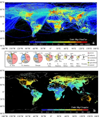
1 180°E 90°N 60°N 30°N 0° 30°S 60°S 90°S

180°W 150°W 120°W 90°W 60°W 30°W 0° 30°E 60°E 90°E 120°E 150°E a Unit: Mg C/km2_/yr 0.1 1 10 100 400 0.01 0 5 50 200 10000 N. America Europe E. Asia S. America W.C. Africa E.-S. Africa Oceania W.C. Asia S. SE. Asia power industry residential vehicles agriculture natural 50% 23% 14% 8.5% 3.2% 0.6% 39% 19% 28% 9.4% 1.1% 3.3% 47% 20% 12% 17% 1.3% 31% 10% 2.5% 2.4% 28% 19% 7.5% 4.3% 60% 12% 6.3% 10% 9.3% 28% 18% 62% 37% 41% 62% 16% 37% 9.5% 24% 16% 180°E 90°N 60°N 30°N 0° 30°S 60°S 90°S

180°W 150°W 120°W 90°W 60°W 30°W 0° 30°E 60°E 90°E 120°E 150°E b 0 0.1 0.5 1 2 5 10 20 100

Unit: Mg C/cap/yr

Fig. 1. Geographic distributions of total and per-capita CO2 emissions from combustion sources at 0.1°×0.1° resolution in 2007 from the PKU-CO2 inventory developed in this study. (a) total CO2 emissions from all

combustion sources and (b) per-capita anthropogenic CO2 emissions excluding shipping and aviation. For total

emission of each region, the relative contribution of each sector is shown in the pie charts in the inset and the total area of each pie is proportional to the emission.

Fig. 1. Geographic distributions of total and per capita CO2

emis-sions from combustion sources at 0.1◦×0.1◦resolution in 2007

from the PKU-CO2inventory developed in this study. (a) Total CO2

emissions from all combustion sources and (b) per capita

energy-related CO2emissions excluding shipping and aviation. For total

emission of each region, the relative contribution of each sector is shown in the pie charts in the inset and the total area of each pie is proportional to the emission.

robust (Fig. S2). A CV in the threshold of 10 % (uniform dis-tribution) was included in the Monte Carlo uncertainty

char-acterization of urban and rural Ecapcalculation.

2.8 Carbon balance of terrestrial ecosystem

For inverse modeling, the spatial distribution of terrestrial

ecosystem CO2fluxes, B(x) where x denotes the spatial

co-ordinate, can be calculated by subtracting fossil fuel CO2

emissions, F (x), from the net land–atmosphere CO2flux

dis-tribution, N (x). The result of the CarbonTracker inversion was used as N (x) for the year 2007 (Peters et al., 2007). Two maps B(x) were calculated as B(x) = N (x) − F (x),

with F (x) being the emission maps either from PKU-CO2or

from NAT-CO2(regridded to 1◦×1◦to match the resolution

of N (x) from CarbonTracker). The difference between the two maps of B(x) obtained with the two F (x) maps was cal-culated to illustrate the effect of using the sub-national (this study) instead of national fuel data (all atmospheric inversion studies) on terrestrial carbon fluxes.

3 Results

3.1 Global fuel consumption and CO2emission map in

2007

According to PKU-FUEL, oil (154 EJ yr−1), coal

(133 EJ yr−1), and natural gas (124 EJ yr−1)

domi-nated global fuel consumptions, followed by biomass

(11.4 EJ yr−1) and solid waste (3.59 EJ yr−1) fuels.

Glob-ally, Fcap was 0.0733 TJ/(cap. × yr), which was primarily

fossil fuel (0.0650 TJ/(cap. × yr)), while energy-related biomass (0.00829 TJ/(cap. × yr)) and solid waste fuels (0.000611 TJ/(cap. × yr)) contributed relatively small

frac-tions. The mean Fcapfor fossil fuels in developed countries

(0.172 TJ/(cap. × yr)) was approximately 4 times of that of developing countries (0.0414 TJ/(cap. × yr)).

PKU-CO2 was developed based on PKU-FUEL using

EFC, and combustion rates of various fuel types. Global CO2

emission from all combustion sources was 11.2 Pg C yr−1

in 2007. The largest contribution was from energy produc-tion (33.8 %), followed by industry (18.0 %), transporta-tion (15.2 %), residential/commercial (14.8 %), and agricul-ture (2.1 %). Wildfires contributed 16.1 % of the total. Fos-sil, biomass, and solid waste fuels emitted 7.83, 3.18, and

0.224 Pg C yr−1, respectively. The estimated fossil fuel

emis-sion of CO2(7.83 Pg C yr−1) is similar to the 7.87 Pg C yr−1

reported by IEA (IEA, 2010c) but lower than the 9.06 Pg

C yr−1from EIA (USEIA, 2010), in which non-fuel-use oil

products were included.

For energy-related (excluding wildfires) fuel combustions,

the global Ecap was 1.51 Mg C/(cap. × yr), with large

vari-ations among and within countries. For example, Ecapwere

0.661 for India, compared to 5.74 Mg C/(cap. × yr) for USA.

Moreover, among the 2373 counties in China, Ecap varied

dramatically from 0.05 to 41.1 Mg C/(cap. × yr), confirming the value of sub-national data down to county level. Emis-sions from individual fuel sub-types are listed in Table 3.

Figure 1 shows the geographical distributions of CO2

emis-sions and Ecap, the relative contributions of the 6 sectors in

9 regions given in the pie charts. Emissions from aviation

(91 Tg C yr−1) and shipping (181 Tg C yr−1) are not included

in the pie charts. Regionally, power generation was the most important sector in North America (38.6 %), Western Eu-rope (46.7 %), and East Asia (50.0 %), while savanna burn-ing dominated in Africa (62.5 %), South America (59.6 %), and Oceania (40.9 %). Emissions from motor vehicles were the second largest contributor in North America (28.3 %)

and Western Europe (16.7 %). In Fig. 1b, Ecapwas high in

the western USA because of relatively high fuel consump-tions for transportation in states with low population densi-ties: Wyoming, North Dakota and Texas (USEIA, 2008). For Alaska and northern Europe, more fuel was consumed for

heating in winter. CO2emission maps separated by the major

fuel categories and sectors are shown in Fig. S3. Information

1 Mexico 79.8% EC-36 71.6% China 61.4% South Africa 59.2% India 59.2% U.S.A. 53.3% Canada 37.8% Turkey 35.7% Brazil 24.2% Australia 17.5% 90°N 60°N 30°N 0° 30°S 60°S 90°S

180°W 150°W 120°W 90°W 60°W 30°W 0° 30°E 60°E 90°E 120°E 150°E 180°E

RD of CO2 emission,% -120 -80 0 80 160 -160 -40 40 120 200 -200 0 0.08 0 0.1 0 0.1 0 0.18 0 0.4 0 0.6 Frequency RD , % -200 0 200 -100

China Mexico U.S.A. India Brazil Australia

100 mean RDs:

Fig. 2. Comparison of CO2 emissions at the scale of sub-nationally disaggregated units (SDUs, e.g. counties, states/provinces, or 0.5 grids) in 45 countries between the sub-nationally (PKU-CO2) and nationally

(NAT-CO2) disaggregated inventories. RDs between the PKU-CO2 and NAT-CO2 inventory were calculated for

all SDUs with sub-national fuel consumption data specially compiled for PKU-CO2 (0.5 ×0.5° grids in

EUCS-36, counties in China, Mexico, and U.S.A., and states/provinces in India, Brazil, Canada, Australia, Turkey, and South Africa). Mean absolute RDs for these countries are listed at the bottom-left of the map. A positive value indicates an underestimation by national data disaggregation. Frequency distributions of RDs for China, Mexico, U.S.A., India, Brazil, and Australia are shown in the bar charts at the bottom.The RD could not be calculated for the countries where sub-national data were not available or not reported, and these areas are marked in black.

Fig. 2. Comparison of CO2emissions at the scale of sub-nationally

disaggregated units (SDUs, e.g., counties, states/provinces, or 0.5◦

grids) in 45 countries between the sub-nationally (PKU-CO2)and

nationally (NAT-CO2) disaggregated inventories. Relative

differ-ences (RDs) between the PKU-CO2and NAT-CO2 inventory are

calculated for all SDUs with sub-national fuel consumption data

specially compiled for PKU-CO₂(0.5◦×0.5◦grids in EUCS-36,

counties in China, Mexico, and USA, and states/provinces in In-dia, Brazil, Canada, Australia, Turkey, and South Africa). Mean ab-solute RDs for these countries are listed at the bottom-left of the map. A positive value indicates an underestimation by national data disaggregation. Frequency distributions of RDs for China, Mexico, USA, India, Brazil, and Australia are shown in the bar charts at the bottom. The RD cannot be calculated for the countries where sub-national data are not available or not reported, and these areas are marked in black.

Table S4, which is valuable for emission prediction and re-gional mitigation policy formation.

3.2 Comparing PKU-CO2with emission maps obtained

from national fuel data (NAT-CO2)

To quantify the improvement expected in PKU-CO2, a

mock-up emission map (NAT-CO2), excluding point (power

sta-tions/natural gas flaring), wildfires, and non-country-specific sources (aviation/shipping), was established using exactly the same method except that nationally aggregated fuel data and proxies were applied for the 45 countries where

PKU-CO2 uses sub-national data. Emissions calculated in the

SDUs of the 45 countries were compared between

PKU-CO2 and NAT-CO2 by calculating a relative difference

RD = (E1−E2)/((E1+E2)/2) where E1 and E2 are mean

emissions in each SDU from PKU-CO2and from the less

ac-curate NAT-CO2, respectively. E1is referred to as the more

accurate value (MAV), since it is derived from actual fuel data in each SDU without minimum proxy and

disaggrega-tion error. By comparison, E2is associated with geographic

bias induced by the disaggregation to smaller scales. In other

words, RD is a metric of how bias of regional CO2emissions

can be reduced by using sub-national fuel data. The larger the

RD value, the more realistic PKU-CO2is over NAT-CO2.

The 45 countries with sub-national fuel data available rep-resented 45, 61, and 69 % of the global total area, population, and fuel consumption, respectively. Within these countries,

CO2emissions were computed from the actual fuel data of

15 197 SDUs instead of from the national fuel data like for-mer studies (Andres et al., 1996; Oda and Maksyutov, 2011). Although residual errors still occurred when disaggregating

the emissions from SDUs to the 0.1◦×0.1◦ grids in

PKU-CO2, these errors should be much smaller than the errors

in-duced by disaggregating the emissions from a country’s total

to 0.1◦×0.1◦grids of NAT-CO2. In fact, the average area of

all SDUs is only 4560 km2, compared to 1 330 108 km2 of

the 45 countries, leading to a significant reduced spatial bias

in the CO2emission distribution. Figure 2 shows the spatial

distribution of RD for the 15 197 SDUs between PKU-CO2

and the less accurate NAT-CO2emission maps. In the 9

coun-tries with county or state/provincial data used in PKU-CO2,

the country averages of RD values in all SDUs range from 17.5 % (Australia) to 79.8 % (Mexico). These large RD val-ues indicate that a substantial reduction of the spatial bias of

CO2emission can be achieved using the sub-national data. It

was also found that the degree of the spatial bias reduction is

larger in countries with higher Fcapheterogeneity (e.g., large

developing countries) or with smaller SDUs (e.g., countries with county fuel data).

3.3 Uncertainty of PKU-CO2

Monte Carlo simulations were applied to estimate

uncertain-ties on CO2 emission maps associated with uncertain fuel

data and uncertain activity data in the spatial disaggregation

process. The result is that R90for global total CO2emission

in 2007 was 4.19 (range 9.11–13.3) Pg C yr−1(see Table 3

for R90of the 64 individual fuel types). For the spatial

dis-tribution of CO2emissions, the absolute and relative

uncer-tainties (R90and R90/M) are shown as maps in Fig. 3. Mean

R90 and R90/M of gridded emissions for the 45 countries

with sub-national data were 62.4 Mg km−2yr−1and 63.2 %

for PKU-CO2, compared to 417 Mg km−2yr−1 and 364 %

for NAT-CO2. This shows that a substantial reduction in the

uncertainty of CO2emission maps can be reached with the

patient effort of collecting sub-national data. In Fig. 3, the

highest R90 values can be found in large countries where

sub-national fuel data are not available, such as Indonesia and Pakistan, and in areas with very high emission densities such as northern China and Western Europe.

3.4 Comparison of PKU-CO2with ODIAC and

VULCAN 2.2 inventories

The PKU-CO2emission map is compared with the ODIAC

one (global fossil fuel, 2007, satellite nightlight-based,

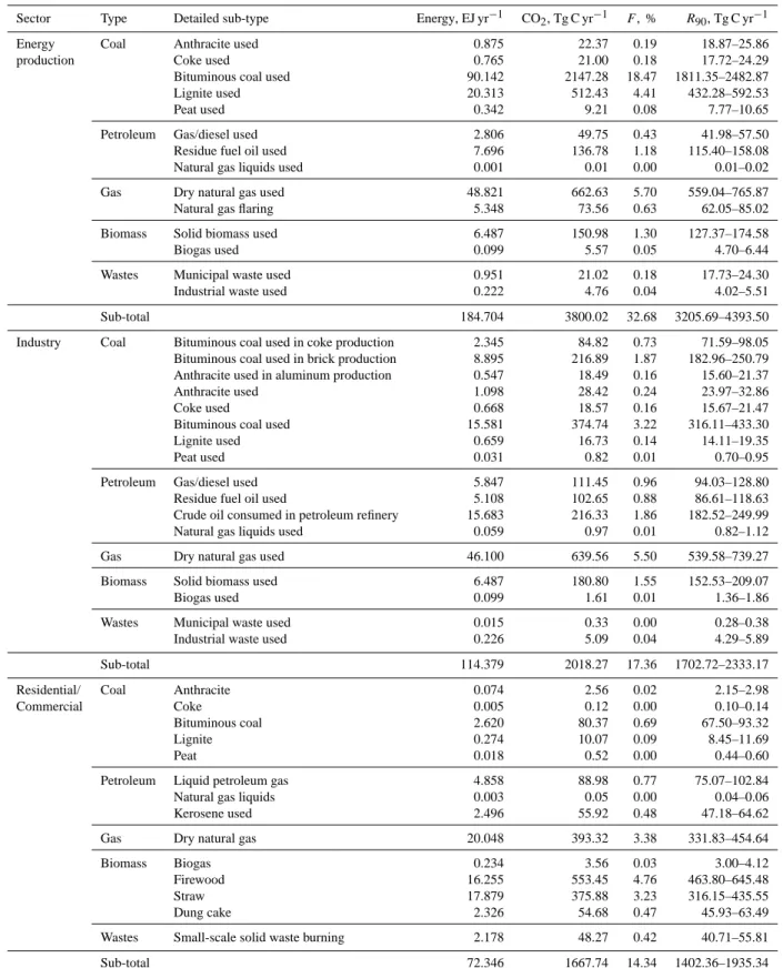
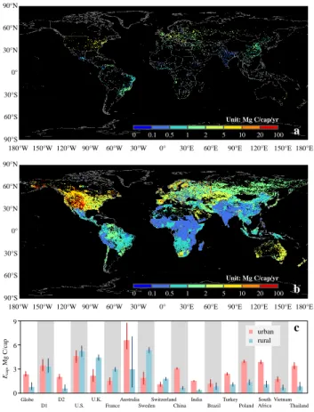
Table 3. Energy and CO2emissions from 64 fuel sub-types and cement production in 2007. Medians and R90(95th minus 5th percentile

range) were used for estimating the emissions and characterizing the uncertainties. CO2emission fractions (F ) are listed for individual fuel

sub-types. The emission from cement production is included in the last two rows so as to provide a complete emission inventory of CO2.

Sector Type Detailed sub-type Energy, EJ yr−1 CO2, Tg C yr−1 F, % R90, Tg C yr−1 Energy Coal Anthracite used 0.875 22.37 0.19 18.87–25.86 production Coke used 0.765 21.00 0.18 17.72–24.29 Bituminous coal used 90.142 2147.28 18.47 1811.35–2482.87 Lignite used 20.313 512.43 4.41 432.28–592.53 Peat used 0.342 9.21 0.08 7.77–10.65 Petroleum Gas/diesel used 2.806 49.75 0.43 41.98–57.50 Residue fuel oil used 7.696 136.78 1.18 115.40–158.08 Natural gas liquids used 0.001 0.01 0.00 0.01–0.02 Gas Dry natural gas used 48.821 662.63 5.70 559.04–765.87 Natural gas flaring 5.348 73.56 0.63 62.05–85.02 Biomass Solid biomass used 6.487 150.98 1.30 127.37–174.58 Biogas used 0.099 5.57 0.05 4.70–6.44 Wastes Municipal waste used 0.951 21.02 0.18 17.73–24.30 Industrial waste used 0.222 4.76 0.04 4.02–5.51 Sub-total 184.704 3800.02 32.68 3205.69–4393.50 Industry Coal Bituminous coal used in coke production 2.345 84.82 0.73 71.59–98.05 Bituminous coal used in brick production 8.895 216.89 1.87 182.96–250.79 Anthracite used in aluminum production 0.547 18.49 0.16 15.60–21.37 Anthracite used 1.098 28.42 0.24 23.97–32.86 Coke used 0.668 18.57 0.16 15.67–21.47 Bituminous coal used 15.581 374.74 3.22 316.11–433.30 Lignite used 0.659 16.73 0.14 14.11–19.35 Peat used 0.031 0.82 0.01 0.70–0.95 Petroleum Gas/diesel used 5.847 111.45 0.96 94.03–128.80 Residue fuel oil used 5.108 102.65 0.88 86.61–118.63 Crude oil consumed in petroleum refinery 15.683 216.33 1.86 182.52–249.99 Natural gas liquids used 0.059 0.97 0.01 0.82–1.12 Gas Dry natural gas used 46.100 639.56 5.50 539.58–739.27 Biomass Solid biomass used 6.487 180.80 1.55 152.53–209.07 Biogas used 0.099 1.61 0.01 1.36–1.86 Wastes Municipal waste used 0.015 0.33 0.00 0.28–0.38 Industrial waste used 0.226 5.09 0.04 4.29–5.89 Sub-total 114.379 2018.27 17.36 1702.72–2333.17 Residential/ Coal Anthracite 0.074 2.56 0.02 2.15–2.98

Commercial Coke 0.005 0.12 0.00 0.10–0.14

Bituminous coal 2.620 80.37 0.69 67.50–93.32 Lignite 0.274 10.07 0.09 8.45–11.69

Peat 0.018 0.52 0.00 0.44–0.60

Petroleum Liquid petroleum gas 4.858 88.98 0.77 75.07–102.84 Natural gas liquids 0.003 0.05 0.00 0.04–0.06 Kerosene used 2.496 55.92 0.48 47.18–64.62 Gas Dry natural gas 20.048 393.32 3.38 331.83–454.64 Biomass Biogas 0.234 3.56 0.03 3.00–4.12 Firewood 16.255 553.45 4.76 463.80–645.48 Straw 17.879 375.88 3.23 316.15–435.55 Dung cake 2.326 54.68 0.47 45.93–63.49 Wastes Small-scale solid waste burning 2.178 48.27 0.42 40.71–55.81 Sub-total 72.346 1667.74 14.34 1402.36–1935.34

Table 3. Continued.

Sector Type Detailed sub-type Energy, EJ yr−1 CO₂, Tg C yr−1 F, % R₉₀, Tg C yr−1 Transport- Petroleum Motor vehicle gasoline 41.862 755.29 6.50 637.21–872.88 ation Aviation gasoline 0.057 1.02 0.01 0.86–1.18 Jet kerosene 4.877 89.56 0.77 75.56–103.51 Motor vehicle gas/diesel 33.334 634.98 5.46 535.73–733.87 Oil used by ocean tanker 2.144 35.94 0.31 23.76–47.86 Oil used by ocean container ships 1.608 26.96 0.23 17.82–35.90 Oil used by bulk and combined carriers 1.488 25.39 0.22 16.78–33.80 Oil used by general cargo vessels 2.600 44.36 0.38 29.33–59.07 Oil used by non-cargo vessels 1.744 30.27 0.26 20.01–40.31 Oil used by auxiliary engines 0.616 10.76 0.09 7.12–14.33 Oil used by military vessels 0.355 7.93 0.07 5.25–10.56 Biomass Liquid biofuels used by vehicles 2.231 42.44 0.36 35.81–49.05 Sub-total 92.916 1704.91 14.66 1405.24–2002.31 Agriculture Petroleum Gas/diesel used in agriculture 6.264 85.27 0.73 71.94–98.55 Wastes Open burning of agriculture waste 4.464 145.03 1.25 121.98–168.04 Sub-total 10.728 230.30 1.98 193.92–266.59 Natural Biomass Biomass burned in forest fires 5.811 193.90 1.67 128.28–258.04 sources Biomass burned in deforestation fires 14.570 489.52 4.21 323.86–651.43 Biomass burned in peat fires 1.372 46.07 0.40 30.48–61.31 Biomass burned in woodland fires 8.527 286.34 2.46 189.44–381.05 Biomass burned in savanna fires 28.620 801.64 6.89 530.29–1066.92 Sub-total 58.900 1817.48 15.63 1202.36–2418.75 Fuel total 533.972 11238.72 96.65 9112.29–13349.65 Cement production 0.129 388.99 3.35 328.32–449.67 Total (fuel and cement production) 534.101 11627.71 100.00 9440.61–13799.32

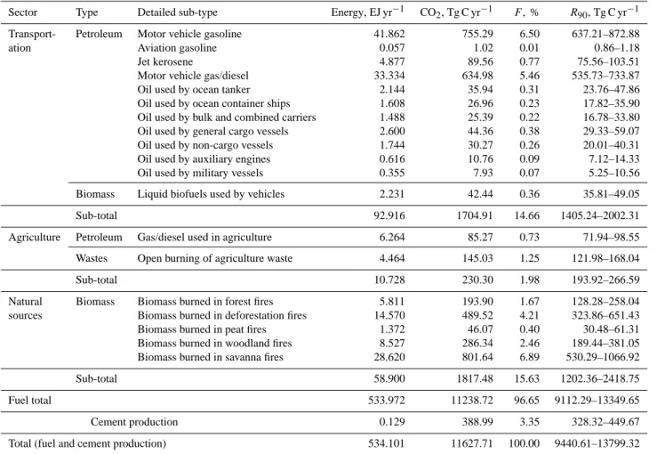
(Oda and Maksyutov, 2011) (Fig. 4). Differences in spatial pattern between the two inventories are large. ODIAC shows more concentrated emissions over urbanized regions with lights. Although a correlation between urban lighting and

CO2emission has been shown on a national basis (Raupach

et al., 2010; Oda et al., 2010), such a relationship is very likely to break down in populated or industrialized rural

ar-eas. For example, large CO2emissions from rural settlements

with high population densities in Sichuan, China, identified

in PKU-CO2 do not appear strongly in satellite nightlights

and ODIAC maps. Similarly, a highly emitting coking in-dustrial zone in Qin county, China, is also associated with negligible nightlight signals (inset of Fig. 4). The

underesti-mation of rural CO2 emissions using nightlight

spatializa-tion has been menspatializa-tioned by Oda et al. (2010). For com-parison, RDs were calculated for all SDUs of the 45

sub-nationally disaggregated countries based on the PKU-CO2

and ODIAC inventory, and E1 (from PKU-CO2)is

consid-ered to be the MAV. The means and standard deviations of the absolute RDs are 113 ± 67.3 % for all SDUs and range from 28.7 ± 29.2 % (8 SDUs in Australia) to 116.7 ± 67.6 % (2373 SDUs in China) for individual countries.

The second inventory to which PKU-CO2was compared is

VULCAN (version 2.2). VULCAN (a 0.1◦×0.1◦ and 1 h

resolution CO2emission inventory for year 2002 (fossil fuel

emissions only) in the USA) is perhaps one of the best emis-sion products in terms of the amount of accurate data entering in its fabrication (Gurney et al., 2009). Over the USA,

VUL-CAN 2.2 is closer to the true emissions than PKU-CO2

be-cause it uses a large number of sectoral “process-based” data

that are not used in PKU-CO2(and not available elsewhere

than in the USA). This is also the reason why we developed a top-down sub-national disaggregation approach. After nor-malization (at the county level to correct for the difference

between 2002 and 2007), PKU-CO2 was compared to the

VULCAN 2.2 over the USA (Fig. 5). RD was calculated for

each 0.1◦ grid point with no MAV assumed, since both

in-ventories are based on county fuel data. Although no sys-tematic skewness is found, more than 30 % of the grid points show a difference larger than a factor of 2 between

PKU-CO2 and VULCAN 2.2. These differences are due to the

fact that detailed information used by VULCAN 2.2 is absent

from PKU-CO2, such as road GIS data and geocoded

commer-1 180°E 90°N 60°N 30°N 0° 30°S 60°S 90°S

180°W 150°W 120°W 90°W 60°W 30°W 0° 30°E 60°E 90°E 120°E 150°E

R90, Mg C/km2_/yr 1 10 100 0.1 50 200 a 0.001 1000 180°E 90°N 60°N 30°N 0° 30°S 60°S 90°S

180°W 150°W 120°W 90°W 60°W 30°W 0° 30°E 60°E 90°E 120°E 150°E

R90/M, % b 36 40 80 200 400 33

30 60 100 300 500

Fig. 3. Geographical distributions of absolute and relative uncertainties of CO2 emissions from combustion sources, excluding shipping and aviation at 0.1°×0.1° resolution. (a) absolute uncertainties as R90 and (b)

relative uncertainties as R90/M, where R90 and M are the 95th minus 5th percentile range and median value

obtained in each grid-point calculated from 1000 Monte Carlo simulations with randomly varied input data. Fig. 3. Geographical distributions of absolute and relative

uncer-tainties of CO2emissions from combustion sources, excluding

ship-ping and aviation at 0.1◦×0.1◦resolution. (a) Absolute

uncertain-ties as R₉₀and (b) relative uncertainties as R₉₀/M, where R₉₀and

M are the 95th minus 5th percentile range and median value

ob-tained in each grid point calculated from 1000 Monte Carlo simula-tions with randomly varied input data.

cial sources, and airports. In addition, for area or nonpoint

sources, CO2 emissions were allocated from the counties

to the USA Census tracts according to the area of residen-tial/commercial/industrial building square footage and then distributed to 10 km × 10 km grids via area-based weighting in VULCAN 2.2, while they were more simply

disaggre-gated to 0.1◦×0.1◦ grids using the 0.8 km × 0.8 km

popu-lation distribution (ORNL, 2008) in PKU-CO2.

In addition, the improvement of the sub-national

disaggre-gation method was also tested by comparing both PKU-CO2

and NAT-CO2with VULCAN 2.2 at various spatial

resolu-tions from 0.1◦ to 4◦ . The average absolute values of RD

between PKU-CO2 and VULCAN 2.2 were much smaller

than those between the NAT-CO2 and VULCAN 2.2

(Ta-ble S5), indicating that most of the reduction of the spatial

bias of CO2emission maps is obtained by using fuel data at

US-states scale, the rest by using realistic activity data like VULCAN 2.2 does.

4 Discussion

4.1 Differences between urban and rural areas

Uneven development of urban and rural areas is a key reason

for Ecap variations within developing countries. It is

inter-esting to compare Ecap between urban and rural areas

us-1 180°E 90°N 60°N 30°N 0° 30°S 60°S 90°S

180°W 150°W 120°W 90°W 60°W 30°W 0° 30°E 60°E 90°E 120°E 150°E a 1 0 5 10 50 100 500 10000 Unit: Mg C/km2_/yr 1000 0 Sichuan Basin Qin county Sichuan Qin 180°E 90°N 60°N 30°N 0° 30°S 60°S 90°S

180°W 150°W 120°W 90°W 60°W 30°W 0° 30°E 60°E 90°E 120°E 150°E b 1 0 5 10 50 100 500 1000 10000 0 Sichuan Basin Qin county Sichuan Qin Unit: Mg C/km2 /yr

Fig. 4. Comparison between ODIAC (a) and PKU-CO2 (b) for fossil fuel emissions excluding shipping and aviation. Emissions in a coking industrial zone in rural area of Qin county, China and heavily populated Sichuan Basin, China are shown in the insets at the bottom-left of the maps. The grids with zero emission are displayed in black.

Fig. 4. Comparison between ODIAC (a) and PKU-CO2(b) for

fos-sil fuel emissions excluding shipping and aviation. Emissions in a coking industrial zone in rural area of Qin county, China, and heav-ily populated Sichuan Basin, China, are shown in the insets at the bottom-left of the maps. The grids with zero emission are displayed in black.

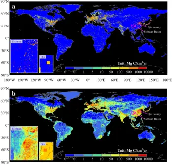
ing sub-nationally spatialized data. In Fig. 6, global fossil

fuel Ecapof urban and rural areas are mapped separately,

to-gether with M and R90 for representative countries.

Glob-ally, Ecapwere 2.41 and 0.799 Mg C/(cap. × yr) as medians

for urban and rural areas, respectively. The gap between

ru-ral and urban Ecapwas found to be very large in developing

countries (2.08 vs. 0.598 Mg C/(cap. × yr)), but small in veloped countries (3.55 vs. 3.41 Mg C/(cap. × yr)). For

de-veloping countries in transition (IMF, 2000), Ecap in urban

areas is close to that of developed countries, but Ecapin rural

areas were not much different from those of other developing

countries. As a typical example, Ecapin China is of 3.28 and

0.691 Mg C/(cap. × yr) in urban and rural areas, respectively.

The large urban–rural Ecap difference in developing

countries is due to uneven socioeconomic development (Satterthwaite, 2009; Dhakal, 2010). Such a difference is a key driver of future emission trends and must be addressed when formulating carbon mitigation policy. For example, China has experienced a rapid urbanization with the urban population rising from 19.6 % in 1980 to 42.2 % in 2007 (World Bank, 2010). A substantial change in economic activ-ity and lifestyle of the new urban settlers is associated with

the factor of 3.2 increase in the country Ecap(IEA, 2010c). It

is anticipated that there will be a rapid increase of CO2

emis-sions from millions of people who will continue to migrate from rural to urban areas in developing countries. Changes in the energy structure in rural areas of developing countries

1 0.002 Emission, kg C/m2_/yr b a C 0.010.05 0.1 1 10 2 Emission, kg C/m2_/yr 10.50.20.100.10.20.51 2 0.002 Emission, kg C/m2_/yr 0.010.05 0.1 1 10 0 -200 F re que n cy ,% 6 2 4 -100 100 200 e 10-1 Vulcan, Mg C/km2 /yr 10-1 ₁₀3 PKU -CO 2 , M g C /k m 2/yr 103 101 101 ₁₀5 R=0.77 105 d RD,% 0

Fig. 5. Comparison between the VULCAN2.2 (a very detailed fossil fuel CO2 process-based emission inventory model, only available over the U.S.A. territory, normalized for individual counties to correct for the difference between 2002 and 2007) and the PKU-CO2 inventory (this study) created at the resolution of 0.1°

over the globe. (a) VULCAN2.2 emissions corrected to year 2007; (b) the PKU-CO2 inventory established for

year 2007; (c) the difference plot between PKU-CO2 and corrected VULCAN2.2. (d) log-scaled scatter plot of

grid-point emissions (84166 grid-points) in PKU-CO2 and corrected VULCAN2.2; (e) Frequency distribution

of relative differences (RD) of grid-point emissions between PKU-CO2 and corrected VULCAN2.2. We do not

expect PKU-CO2 to be more realistic than the VULCAN2.2 inventory, but this comparison is shown to

illustrate how PKU-CO2 approaches VULCAN2.2 best product over a region where the comparison is

possible.

Fig. 5. Comparison between the VULCAN 2.2 (a very detailed

fos-sil fuel CO2 process-based emission inventory model, only

avail-able over the USA territory, normalized for individual counties to correct for the difference between 2002 and 2007) and the

PKU-CO2inventory (this study) created at the resolution of 0.1◦over the

globe. (a) VULCAN 2.2 emissions corrected to year 2007; (b) the

PKU-CO2inventory established for the year 2007; (c) difference

plot between PKU-CO₂and corrected VULCAN 2.2; (d) log-scaled

scatter plot of grid-point emissions (84166 grid points) in PKU-CO2

and corrected VULCAN 2.2; (e) frequency distribution of relative

differences (RDs) of grid-point emissions between PKU-CO2and

corrected VULCAN 2.2. We do not expect PKU-CO2to be more

realistic than the VULCAN 2.2 inventory, but this comparison is

shown to illustrate how PKU-CO2approaches VULCAN 2.2 best

product over a region where the comparison is possible.

are also taking place with improved stoves, biogas, liquid petroleum gas, and electric appliances being used increas-ingly (Cai and Jiang, 2008). Although this trend could im-prove energy efficiency and reduce emissions of air pollu-tants, the replacement of traditional biomass fuels by fossil

fuels and electricity may result in greater Ecapin rural areas

as well (Solomon et al., 2007).

4.2 Impact of PKU-CO2 emission maps on terrestrial

CO2flux maps derived from an inversion

The spatial distribution of terrestrial CO2 fluxes inferred

using atmospheric CO2 measurements and inverse models

remains uncertain (affected with biases), partly due to the lack of emission information with high spatial and tempo-ral resolutions (Lauvaux et al., 2009). Peylin et al. (2011) investigated the influence of using different fossil fuel

emis-sion inventories on the simulation of CO2in the atmosphere

in Europe, and pointed out an urgent need to improve the

spatially and temporally resolved CO2 emission inventory.

Therefore, reducing the uncertainty of CO2emission maps

F (x)helps to reduce uncertainty of terrestrial carbon fluxes

B(x)in inversions (see Sect. 2.8 for definitions). PKU-CO2

and NAT-CO2were compared for deducing B(x) using the

CarbonTracker inversion of the net fossil + terrestrial CO2

flux, N (x) (NOAA, 2010). B(x) calculated by subtracting

either PKU-CO2or NAT-CO2maps from N (x) are shown in

1 0 0.1 0.5 1 2 5 10 20 100 180°E 90°N 60°N 30°N 0° 30°S 60°S 90°S

180°W 150°W 120°W 90°W 60°W 30°W 0° 30°E 60°E 90°E 120°E 150°E Unit: Mg C/cap/yr a 0 0.1 0.5 1 2 5 10 20 100 180°E 90°N 60°N 30°N 0° 30°S 60°S 90°S

180°W 150°W 120°W 90°W 60°W 30°W 0° 30°E 60°E 90°E 120°E 150°E Unit: Mg C/cap/yr b 9 0 6 Globe 3 D1 U.S. Australia D2 India France Switzerland Poland Turkey Vietnam Sweden China Thailand U.K. Ecap , Mg C /cap c South Africa Brazil urban rural

Fig. 6. Comparison in per-capita fossil fuel CO2 emissions between urban and rural areas. (a) urban Ecap map,

(b) rural Ecap map, and (c) Ecap as M and R90 from the Monte Carlo simulations for 14 representative countries,

all developed countries (D1), all developing countries (D2), and the globe. For the Monte Carlo simulations, both variations in PKU-CO2 and urban-rural classification criteria (uniform distribution, ±10%) were taken

into consideration.

Fig. 6. Comparison in per capita fossil fuel CO2emissions (Ecap)

between urban and rural areas: (a) urban Ecapmap, (b) rural Ecap

map, and (c) Ecapas M and R90from the Monte Carlo simulations

for 14 representative countries, all developed countries (D1), all de-veloping countries (D2), and the globe. For the Monte Carlo

simu-lations, both variations in PKU-CO₂and urban–rural classification

criteria (uniform distribution, ±10 %) are accounted for.

Fig. 7a. With the PKU-CO2emission inventory, a different

pattern of terrestrial CO2sources and sinks is obtained. To

test the effect of sub-national disaggregation of emissions on

B(x)distribution, differences in the B(x) calculated based on

PKU-CO2and NAT-CO2are shown in Fig. 7b. The mean

ab-solute difference in B(x) by country is 52.2 (Mexico), 40.4 (China), 28.3 (USA), 17.9 (India), 3.05 (Brazil), and 0.681

(Australia) g C km−2yr−1. This simple application of

PKU-CO2here serves only to illustrate that using a CO2emission

map based on sub-national disaggregation method has a large indirect influence on B(x). In a future study, one should

pre-scribe PKU-CO2and its uncertainty to an inversion system

to correct both F (x) and B(x) using atmospheric CO2

obser-vations.

5 Conclusions

PKU-FUEL and PKU-CO2appear to be the first global

1 90°N 60°N 30°N 0° 30°S 60°S 90°S

180°W 150°W 120°W 90°W 60°W 30°W 0° 30°E 60°E 90°E 120°E 150°E 180°E

a B(x): g C/km2_/yr -100 -50 5 100 -250 -5 0 50 250 90°N 60°N 30°N 0° 30°S 60°S 90°S

180°W 150°W 120°W 90°W 60°W 30°W 0° 30°E 60°E 90°E 120°E 150°E 180°E

b

B(x): g C/km2 /yr -100 -50 5 100 -250 -5 0 50 250

Fig. 7. Geographic distribution of terrestrial ecosystem carbon flux deduced by subtracting from the net

land-atmosphere carbon flux in an atmospheric inversion CarbonTracker. (a) carbon balance based on the PKU-CO2 inventory, and the negative (positive) values are corresponding to carbon sinks (sources), and (b)

map of differences in terrestrial ecosystem carbon fluxes for sub-nationally disaggregated units (SDUs) based on the PKU-CO2 inventory and the (regionally) less accurate NAT-CO2 inventory relying on national fuel data

only for the 45 countries. This result depends on the inversion model used and the two maps are shown only as an example.The RD could not be calculated for the countries where sub-national data were not available or not reported, and these areas are displayed in black.

Fig. 7. Geographic distribution of terrestrial ecosystem CO2fluxes

deduced by subtracting from the net land–atmosphere carbon flux in an atmospheric inversion CarbonTracker. (a) Carbon balance based

on the PKU-CO2inventory, and the negative (positive) values

cor-respond to carbon sinks (sources), and (b) map of differences in terrestrial ecosystem carbon fluxes for sub-nationally disaggregated

units (SDUs) based on the PKU-CO2 inventory and the

(region-ally) less accurate NAT-CO2inventory relying on national fuel data

only for the 45 countries. The fluxes are not adjusted for other GHG exchange and crop harvest. This result also depends on the inver-sion model used, and the two maps are shown only as an example. The RD could not be calculated for the countries where sub-national data were not available or not reported, and these areas are displayed in black.

and CO2 emission maps, for which an uncertainty is

esti-mated. The major improvements of PKU-CO2 over

previ-ous inventories are as follows: (1) a large database of sub-national fuel consumptions was used for 45 major countries,

which explicitly accounts for uneven distributions of Fcap

and Ecapwithin these countries; (2) fossil, biomass, and solid

waste fuels were included and categorized into 64 types in

6 economic sectors, and (3) uncertainties of the CO2

emis-sion maps were quantified. The relative uncertainty range

(R90/M) of CO2 emission could be reduced from 364 % to

63.2 % by using the sub-national disaggregation. In the 9 countries with sub-national data of different levels available,

the spatial distortion of CO2emissions by using a nationally

disaggregation method can be reduced by 17.5–79.8 %, indi-cating a substantial reduction of the spatial bias. It was also found that the degree of spatial bias reduction is larger in countries with a higher degree of imbalance or with smaller SDUs applied.

The inventory can be further improved by compiling more sub-national fuel consumption data for other large countries. Inventories with temporal resolutions, both intra- and

inter-annual, are also needed. The significant difference in CO2

emissions between urban and rural areas in transition coun-tries suggests that more studies on the effect of rapid

urban-ization on CO2emissions should be addressed. PKU-FUEL

is ready to be used for estimating emissions of other green-house gases, black carbon, and various air pollutants, which can help us to improve our understanding on combustion-related climate forcing and health impact. In the future, sub-national data are recommended to be reported by large coun-tries with high differences in per capita fuel consumption, so as to reduce spatial bias in IPCC GHG reporting.

List of abbreviations

CO2: carbon dioxide

SDM: sub-national disaggregation method

EF: emission factor

Fcap: per capita fuel consumption

Ecap: per capita CO2emission

GOSAT: Japanese Greenhouse gases

Observing SATellite Project

PKU: Peking University

PKU-FUEL: Peking University Fuel Inventories

PKU-CO2: Peking University CO2Inventories

EUCS-36: the 36 European countries

with sub-national data

SDU: sub-nationally disaggregated unit

Nat-CO2: a mock-up inventory generated based on

the national fuel data and disaggregation

CO: carbon monoxide

NOx: nitrogen oxide

CARMA: Carbon Monitoring for Action

CV: coefficient of variation

RD: relative difference

R90: 95th minus 5th percentile range

M: median

R90/ M: the ratio of R90to median

ODIAC: Open source Data Inventory of

Anthropogenic CO2emission

IEA: International Energy Agency

EDGAR: The Emissions Database for Global

Atmospheric Research

MAV: more accurate value

Supplementary material related to this article is

available online at: http://www.atmos-chem-phys.net/13/ 5189/2013/acp-13-5189-2013-supplement.zip.

Acknowledgements. Funding for this study was provided by the

CarbonTracker 2010 results were provided by NOAA ESRL, Boulder, Colorado, USA (http://carbontracker.noaa.gov). We thank Tomohiro Oda (NOAA Earth System Research Lab, USA) and Shamil Maksyutov (National Institute for Environmental Studies, Japan) for providing the original data of ODIAC and valuable com-ments, Christopher D. Elvidge (NOAA National Geophysical Data Center, USA) for helping us to retrieve natural gas flaring data, and Brian Reid (University of East Anglia, UK) and Matthew J. Mc-Grath (Laboratoire des Sciences du Climat et de l’Environnement, France) for valuable comments and proof-reading.

Edited by: P. Monks

References

Andreae, M. O. and Merlet, P.: Emission of trace gases and aerosols from biomass burning, Global Biogeochem. Cy., 15, 955–966, 2001.

Andres, R. J., Marland, G., Fung, I. E., and Matthews, E. A.:

1◦×1◦distribution of carbon dioxide emissions from fossil fuel

consumption and cement manufacture, 1950-1990, Global Bio-geochem. Cy., 10, 419–429, 1996.

American Petroleum Institute (API): Compendium of Greenhouse Gas Emissions Estimation Methodologies for the Oil and Gas Industry, Pilot Test Version, available at: http://www.api.org/ environment-health-and-safety/climate-change/whats-new/ compendium-ghg-methodologies-oil-and-gas-industry, 2001. Australian Bureau of Agricultural and Resource Economics and

Sciences (ABES): Energy in Australia 2008, available at: http: //www.abares.gov.au/publications, 2008.

Bocquet, M.: Grid resolution dependence in the reconstruction of an atmospheric tracer source, Nonlinear Proc. Geophy., 34, 521– 529, 2005.

Bond, T. C., Streets, D. G., Fernandes, S. D., Nelson, S. M., Yarber, K. F., Woo, J.-H., and Klimont, Z.: A technology-based global inventory of black and organic carbon emis-sions from combustion, J. Geophys. Res. Atmos., 109, D14203, doi:10.1029/2003JD003697, 2004.

Brazil Energy Ministry: Brazil Energy Statistics, available at: http: //www.mme.gov.br/mme, 2010.

British Petroleum (BP): Statistical Review of World Energy-2007, available at: http://www.bp.com, 2008.

Cai, J. and Jiang, Z.: Changing of energy consumption patterns from rural households to urban households in China: an example from Shaanxi Province, China, Renew. Sust. Energ. Rev., 12, 1667– 1680, 2008.

Cao, G. L., Zhang, X. Y., Wang, D., and Zheng, F. C.: Inventory of emissions of pollutants from open burning crop biomass, J. Agr. Environ. Sci. 24, 800–804, 2005.

Centre on Emission Inventories and Projections (CEIP): Emissions as used in EMEP models, available at: http://www.ceip.at (last access: 14 August 2012), 2011.

Ciais, P., Paris, J. D., Marland, G., Peylin, P., Piao, S. L., Levin, I., Pregger, T., Scholz, Y., Friedrich, R., Rivier, L., Houwelling, S., Schulze, E. D., and members of the CARBOEUROPE SYN-THESIS TEAM (1): The European carbon balance, Part 1: fossil fuel emissions, Global Change Biol., 16, 1395–1408, 2010.

Davis, S. J., Caldeira, K., and Matthews, H. D.: Future CO₂

emis-sions and climate change from existing energy infrastructure,

Science, 329, 1330–1332, 2010.

Dhakal, S.: GHG emissions from urbanization and opportunities for urban carbon mitigation, Curr. Opin. Env. Sust., 2, 277–283, 2010.

Elvidge, C. D., Ziskin, D., Baugh, K. E., Tuttle, B. T., Ghosh, T., Pack, D. W., Erwin, E. H., and Zhizhin, M.: A fifteen year record of global natural gas flaring derived from satellite data, Energies, 2, 595–622, 2009.

Environment Canada/Natural Resource Canada: State Energy Statistics 2007, available at: www.nrcan.gc.ca, 2010.

Equasis: The world merchant fleet in 2007 (Lisbon), available at: http://www.equasis.org/EquasisWeb/public/HomePage (last ac-cess: 14 August 2012), 2008.

European Commission: Joint Research Centre (JRC)/Netherlands Environmental Assessment Agency (PBL). Emission Database for Global Atmospheric Research (EDGAR), release version 4.2. http://edgar.jrc.ec.europa.eu, 2011.

Eyers, V., Kohler, H. W., van Aardenne, J., and Lauer, A.: Emissions from international shipping: 1. The last 50 years, J. Geophys. Res., 110, D17305, doi:10.1029/2004JD005619, 2005.

Food and Agriculture Organization of the United Nations (FAO): FAOSTAT food and agriculture statistics, available at: http:// faostat.fao.org/default.aspx, 2010.

Friedl, M. A., Mclver, D. K., Hodges, J., Zhang, X. Y., Muchoney, D., Strahler, A. H., Woodcock, C. E., Gopal, S., Schneider, A., Cooper, A., Baccini, A., Gao, F., and Schaaf, C.: Global land cover mapping from MODIS: algorithms and early results, Re-mote Sens. Environ., 83, 287–302, 2002.

Gurney, K. R., Mendoza, D. L., Zhou, Y., Fischer, M. L., Miller, C. C., Geethakumar, S., and de la Rue du Can, S.: High resolution

fossil fuel combustion CO2emission fluxes for the United States,

Environ. Sci. Technol., 43, 5535–5541, 2009.

Intergovernmental Panel on Climate Change (IPCC): Revised 1996 IPCC Guidelines for National Greenhouse Gas Inventories, Ref-erence Manual (Volume 3), United Nations Environment Pro-gramme, the Organization for Economic Co-operation and De-velopment, the International Energy Agency, IPCC, available at: http://www.ipcc-nggip.iges.or.jp/public/gl/invs1.htm, 1996. International Energy Agency (IEA): Energy Statistics and Balances

of OECD Countries, 2007–2008, Paris, 2010a.

International Energy Agency (IEA): Energy Statistics and Balances of Non-OECD Countries, 2007–2008, Paris, 2010b.

International Energy Agency (IEA): CO2 Emission From Fuel

Combustion-2011 Highlights, Paris, 2010c.

International Monetary Fund (IMF): Transition Economies: An IMF Perspective on Progress and Prospects, available at: http: //www.imf.org/external/np/exr/ib/2000/110300.htm, 2000. Johnson, M., Edwards, R., Frenk, C. A., and Masera, O.: In-field

greenhouse gas emissions from cookstoves in rural Mexican households, Atmos. Environ., 42, 1206–1222, 2008.

Lauvaux, T., Pannekoucke, O., Sarrat, C., Chevallier, F., Ciais, P., Noilhan, J., and Rayner, P. J.: Structure of the transport

uncer-tainty in mesoscale inversions of CO₂ sources and sinks

us-ing ensemble model simulations, Biogeosciences, 6, 1089–1102, doi:10.5194/bg-6-1089-2009, 2009.

Lee, S., Baumann, K., Schauer, J. J., Sheesley, R. J., Naeher, L. P., Meinardi, S., Blake, D. R., Edgerton, E. S., Russell, A. G., and Clements, M.: Gaseous and particulate emissions from pre-scribed burning in Georgia, Environ. Sci. Technol., 39, 9049–