Impact of brine-induced stratification on the glacial carbon cycle

HAL Id: hal-02891945

https://hal.archives-ouvertes.fr/hal-02891945

Submitted on 28 Jul 2020

HAL is a multi-disciplinary open access

archive for the deposit and dissemination of

sci-entific research documents, whether they are

pub-lished or not. The documents may come from

teaching and research institutions in France or

abroad, or from public or private research centers.

L’archive ouverte pluridisciplinaire HAL, est

destinée au dépôt et à la diffusion de documents

scientifiques de niveau recherche, publiés ou non,

émanant des établissements d’enseignement et de

recherche français ou étrangers, des laboratoires

publics ou privés.

carbon cycle

Nathaëlle Bouttes, D. Paillard, Didier Roche

To cite this version:

Nathaëlle Bouttes, D. Paillard, Didier Roche. Impact of brine-induced stratification on the glacial

carbon cycle. Climate of the Past, European Geosciences Union (EGU), 2010, 6 (5), pp.575-589.

�10.5194/cp-6-575-2010�. �hal-02891945�

www.clim-past.net/6/575/2010/ doi:10.5194/cp-6-575-2010

© Author(s) 2010. CC Attribution 3.0 License.

Climate

of the Past

Impact of brine-induced stratification on the glacial carbon cycle

N. Bouttes1, D. Paillard1, and D. M. Roche1,2

1_{Laboratoire des Sciences du Climat et de l’Environnement, IPSL-CEA-CNRS-UVSQ, UMR 8212, Centre d’Etudes de} Saclay, Orme des Merisiers bat. 701, 91191 Gif Sur Yvette, France

2_{Faculty of Earth and Life Sciences, Section Climate Change and Landscape dynamics, Vrije Universiteit Amsterdam,} De Boelelaan, 1085, 1081 HV Amsterdam, The Netherlands

Received: 26 March 2010 – Published in Clim. Past Discuss.: 26 April 2010

Revised: 23 August 2010 – Accepted: 31 August 2010 – Published: 15 September 2010

Abstract. During the cold period of the Last Glacial Maxi-mum (LGM, about 21 000 years ago) atmospheric CO2was around 190 ppm, much lower than the pre-industrial con-centration of 280 ppm. The causes of this substantial drop remain partially unresolved, despite intense research. Un-derstanding the origin of reduced atmospheric CO2 during glacial times is crucial to comprehend the evolution of the different carbon reservoirs within the Earth system (atmo-sphere, terrestrial biosphere and ocean). In this context, the ocean is believed to play a major role as it can store large amounts of carbon, especially in the abyss, which is a car-bon reservoir that is thought to have expanded during glacial times. To create this larger reservoir, one possible mecha-nism is to produce very dense glacial waters, thereby strati-fying the deep ocean and reducing the carbon exchange be-tween the deep and upper ocean. The existence of such very dense waters has been inferred in the LGM deep Atlantic from sediment pore water salinity and δ18O inferred temper-ature. Based on these observations, we study the impact of a brine mechanism on the glacial carbon cycle. This mech-anism relies on the formation and rapid sinking of brines, very salty water released during sea ice formation, which brings salty dense water down to the bottom of the ocean. It provides two major features: a direct link from the sur-face to the deep ocean along with an efficient way of set-ting a strong stratification. We show with the CLIMBER-2 carbon-climate model that such a brine mechanism can ac-count for a significant decrease in atmospheric CO2and con-tribute to the glacial-interglacial change. This mechanism can be amplified by low vertical diffusion resulting from the brine-induced stratification. The modeled glacial

dis-Correspondence to: N. Bouttes

(nathaelle.bouttes@lsce.ipsl.fr)

tribution of oceanic δ13C as well as the deep ocean salinity are substantially improved and better agree with reconstruc-tions from sediment cores, suggesting that such a mechanism could have played an important role during glacial times.

1 Introduction

Proxy data suggest that the climate of the Last Glacial Max-imum (LGM, about 21 000 years ago) was very cold (−2 to −6◦C in the Southern Ocean surface (MARGO Project Members, 2009)) with huge Northern Hemisphere ice sheets (Peltier, 2004). The associated carbon cycle was character-ized by low atmospheric CO2 concentrations of ∼190 ppm (Monnin et al., 2001) and very negative deep ocean δ13C. The latter is based on the stable carbon isotopic composition (δ13C) of benthic foraminifera which is assumed to reflect the δ13C of total dissolved inorganic carbon (DIC) in bottom waters.

The Atlantic δ13C reached low values down to −0.8‰ in the deep ocean participating in a higher upper to deep oceanic gradient (Duplessy et al., 1988; Curry and Oppo, 2005; K¨ohler and Bintanja, 2008). The mean upper (−2000 m to 0 m) to deep (−5000 m to −3000 m) gradient in the Atlantic, (noted 1δ13Catl), was about 1.2‰ in the Atlantic, compared to only 0.4‰ during the pre-industrial.

LGM climate can be explained by the extended ice sheets in connection with a different orbital configuration (Berger, 1978) and lower CO2 (Jahn et al., 2005). To ex-plain the crucial question of the low glacial CO2 numer-ous hypotheses have been proposed. Some of them im-ply changes of physical mechanisms such as modifications of sea ice coverage (Stephens and Keeling, 2000) or winds (Toggweiler et al., 2006). Many have focused on enhancing

or making more efficient the marine biology, for example through higher C/P ratio (Broecker and Peng, 1982), iron fertilization (Martin, 1990), a shift of dominant plankton species (Archer and Maier-Reimer, 1994), larger nutrients availability (Matsumoto et al., 2002), or modified rain ratio (Brovkin et al., 2007). Other studies have involved coral reef fluctuations (Berger, 1982; Opdyke and Walker, 1992), or oceanic chemistry with carbonate compensation (Broecker and Peng, 1987). But most only have a small impact on CO2 compared to the glacial-interglacial change, or would require unrealistic modifications to become dominant (Archer et al., 2000, 2003; Kohfeld et al., 2005; Menviel et al., 2008b). Moreover, it has remained especially difficult to correctly simulate simultaneously the very negative δ13C in the deep ocean inferred from marine sediment cores, although part of the change is due to the glacial reduced terrestrial biosphere which releases light12C leading to a reduction of the global mean oceanic δ13C (K¨ohler et al., 2010). Additionally, the strong link between Antarctic temperatures and atmospheric CO2variations (Luthi et al., 2008) suggests that mechanisms closely tied to Southern Ocean surface processes are likely to be dominant in controlling atmospheric CO2variability.

The general consensus is that the ocean is at the core of the solution regarding LGM CO2. It is the biggest carbon reser-voir active on the short time scale studied (a few thousand years) and the only one that could increase during glacial times, since the other two reservoirs, i.e., the atmosphere (Monnin et al., 2001) and terrestrial biosphere (Bird et al., 1994; Crowley, 1995), were both reduced. Observations in-dicate that the deep glacial ocean was much saltier and colder than today (Adkins et al., 2002), thus more stratified in the abyss. Such a deep stratification has important impacts on the ocean’s circulation and carbon cycle, as pointed out by climate models of different complexities (Toggweiler, 1999; Paillard and Parrenin, 2004; K¨ohler et al., 2005a; Bouttes et al., 2009; Tagliabue et al., 2009). In particular, deep stratification is required to reconcile δ13C (Bouttes et al., 2009; Tagliabue et al., 2009). However, only box models could significantly reduce atmospheric CO2when prescrib-ing a reduced Southern ventilation (Watson and Garabato, 2005). With models of higher complexity (Bouttes et al., 2009; Tagliabue et al., 2009) the induced CO2drop remained too small which highlights the need of another mechanism that would still maintain the benefits of deep stratification (deep negative δ13C values) while reducing CO2more dras-tically.

Here we test the impact of the formation and rapid deep sinking of brines, i.e. very salty waters rejected during sea ice formation, on the glacial carbon cycle. The role of brines has been previously proposed as an explanation for the reduced Southern ventilation (Paillard and Parrenin, 2004; K¨ohler et al., 2005a; Watson and Garabato, 2005), but they were not explicitly simulated. Instead, the proposed effect of re-ducing the ventilation was tested by imposing lower mixing in box models only. Here we directly test this mechanism

with a more complex model which physically includes ad-vection and diffusion in the ocean and thus is able to repro-duce the dynamical effect of brines. Because they are en-riched in salt, these “pockets of water” are very dense. In the modern Antarctic they are generally mixed with fresh water from ice shelf melting (Joughin and Padman, 2003). How-ever, during the glacial periods the sea level progressively fell (down to about 120 m at the Last Glacial Maximum) and the northward Antarctic ice sheet extent resulted in a progressive reduction of the shelf slope (Ritz et al., 2001) where mod-ern waters are mixed. Tidal dissipation, which is important in today’s mixing, would then seriously decrease. Accord-ingly, the brine signal, which is diluted today, would be more preserved at the LGM. Furthermore, the sea ice formation location would also shift northward and closer to the conti-nental shelf break. The preserved brine-dense water, whose volume was increased because of enhanced sea ice forma-tion, would arrive at the shelf break and then flow quickly down the slope (helped by thermobaricity and supercritical flux properties) (Foldvik et al., 2004). This mechanism (re-ferred herein thereafter as the brine mechanism) provides two major features: a direct link from the surface to the deep ocean and an effective physical way of achieving a strong stratification. In this study we test its impact on the carbon cycle and compare the modeled results to atmospheric CO2, oceanic δ13C and salinity data inferred from ice core and ma-rine sediment cores.

2 Methods

2.1 CLIMBER-2 model

The brine mechanism has been implemented and tested in CLIMBER-2, an intermediate complexity climate model (Petoukhov et al., 2000) well suited for the long term sim-ulations we run. Indeed, the simsim-ulations are run for 20 000 years to ensure the equilibrium of the carbon cycle. More-over we realize an ensemble of about 100 simulations to test the mechanism, which would be unfeasible with a general circulation model (GCM) in a reasonable amount of time. The intermediate complexity model, although simpler than a state of the art OGCM, includes the main known processes and mechanisms and computes the dynamics of the oceanic circulation contrary to box models. Furthermore, like GCMs, CLIMBER-2 does not exhibit box model sensitivity to high-latitude sea ice or presumably stratification (Archer et al., 2003). Additionally, the model compares favourably with a state of the art OGCM and gives the same response in terms of carbon cycle when the circulation is arbitrarily modified (Tagliabue et al., 2009).

CLIMBER-2 has a coarse resolution of 10◦in latitude by 51◦in longitude in the atmosphere, and 21 depth levels by 2.5◦ latitude in the zonally averaged ocean, which is pre-cise enough to take into account geographical changes, while

allowing the model to be fast enough to run the long simu-lations considered. The model is composed of various mod-ules simulating the ocean, the atmosphere, and the continen-tal biosphere dynamics. No sediment model is included, the model thus does not take into account the carbonate com-pensation mechanism. CLIMBER-2 has already been used and evaluated in previous studies (Ganopolski et al., 2001a; Brovkin et al., 2002a,b, 2007; Bouttes et al., 2009). As the model version used explicitly computes the evolution of the carbon cycle and carbon isotopes (such as δ13C) in every reservoirs, it allows us to compare the model output with data from sediment cores. In the glacial simulations three boundary conditions are simultaneously imposed: the ice sheets (Peltier, 2004), the solar insolation (Berger, 1978), and the atmospheric CO2concentration for the radiative forc-ing (190 ppm, not used in the carbon cycle part of the model) (Monnin et al., 2001). To account for the glacial sea level fall of about 120 m, salinity and nutrients (NO−₃ and PO2−₄ ) mean concentrations are increased by 3.3%.

2.2 Implementation of brines in the CLIMBER-2 model When sea ice is formed, a flux of ions is released into the ocean as sea ice is mostly composed of fresh water (Wakat-suchi and Ono, 1983; Rysgaard et al., 2007, 2009). Be-cause the underlying water is then enriched in salt it becomes denser and can thus sink and transport salt to deeper waters. The rejection of salt by sea ice formation plays an impor-tant role in the formation of deep water, as it is the case for the Antarctic Bottom Water (AABW) which has been stud-ied for a few decades (Foster and Carmack, 1976; Whitworth and Nowlin, 1987; Foldvik et al., 2004; Nicholls et al., 2009). The brine mechanism has been mostly observed in details in the Northern Hemisphere oceans (Haarpaintner et al., 2001; Shcherbina et al., 2003; Skogseth et al., 2004, 2008), where measures are easier than in the Southern Ocean. For in-stance, measures in the Arctic fjords indicate that approxi-mately 78% of the brine-enriched shelf water was released out of the fjord in the Norwegian Sea (Haarpaintner et al., 2001), i.e. around 62% of the salt flux rapidly released by sea ice formation (the first rapid salt release is ∼82% of the total salt flux rejected by sea ice formation). The impact of the brine formation on the concentration of other geochem-ical variables, especially dissolved inorganic carbon (DIC) has also been studied and it has been shown that DIC is re-jected together with brine from growing sea ice (Rysgaard et al., 2007, 2009). Besides, numerical studies of this local mechanism show that the topography plays an important role in the transport of salt (Kikuchi et al., 1999).

Thus although today the brine formation around Antarc-tica does not affect the bottom waters (Toggweiler and Samuels, 1995), the formation and sinking of brines is a mechanism that can be observed and studied in some places of the modern ocean and that strongly depends on local con-ditions. The inferred higher salinity in the glacial Southern

Ocean seems to indicate that enhanced brine formation and sinking could well have taken place around Antarctica during glacial conditions, which should be tested.

In order to assess the potential impact of the sinking of brines on the carbon cycle we need to use a global carbon-climate model. Yet the spatial resolution of such models, even state of the art GCMs, is too large to resolve the brine sink, requesting a parameterization. We thus develop a sim-ple parameterization for this mechanism. The simplicity of the scheme used permits a first evaluation of such a mech-anism and allows a separation of the different processes to understand the reasons of the changes observed.

The sinking of brines initially depends on the amount of salt rejected which is determined by the rate of sea ice for-mation. In CLIMBER-2, sea ice formation is computed by a one layer thermodynamic sea ice model with a simple param-eterization for horizontal ice transport (Brovkin et al., 2007). The sea ice extent is increased in winter in agreement with proxy data (Gersonde et al., 2005) although during summer sea ice extent is also increased contrary to the data which indicate a sea ice covered area similar to the modern one.

During the formation of sea ice, in the standard version of CLIMBER-2 only the flux of salt (FS) was considered. It is usually a good approximation on the first order, yet the release of other ions and dissolved gases could be of impor-tance for this study. Hence we have added the same process as the release of salt for the other ions and dissolved gases simulated in the model (dissolved inorganic carbon (DIC), al-kalinity (ALK), nutrients, dissolved organic carbon, oxygen, DI13C, DI14C). As a first approximation the surface oceanic cell is enriched in these geochemical variables in the same proportion as salt as it has been observed to be not very dif-ferent on the first order (Rysgaard et al., 2007, 2009). The flux (FX) of any geochemical variable X rejected during sea

ice formation to the surface ocean is then:

FX= FS

Ssurface

·Xsurface (1)

With FS the flux of salt, Ssurfacethe surface salinity, and

Xsurface the surface concentration of any geochemical vari-able.

This process is active in all simulations, though it has a small impact on the standard pre-industrial and LGM simu-lations (atmospheric CO2is changed by less than 5 ppm).

In the standard version of CLIMBER-2 when sea ice is formed all the salt is released in the corresponding surface oceanic cell, which is relatively large according to the coarse resolution of the model and thus dilutes the brine signal. In the brine simulations, a fixed fraction (frac) of this salt flux (and of the other ions flux) will form the sinking brines (Fig. 1a). This fraction frac can be set to 0 when none of the salt sinks to the bottom of the ocean (standard version of the model) and 1 when all the salt is used in the brine mech-anism. The very salty (thus dense) brine water sinks to the bottom of the ocean where it modifies the concentration of

ions flux

sea ice formation

(1-frac) x FX

sea ice melting

fresh water flux

surface

bottom

frac x FX

brines

salty dense water

a

b

Fig. 1. (a) Brine sinking mechanism scheme and (b) Potential density difference between the

deep Atlantic ocean (between -5000 m and -3000 m) and the upper Atlantic ocean (between

-2000 m and 0 m) as a function of the fraction of salt released by sea ice formation used for

the brine mechanism (fraction of salt f rac, 0 ≤ f rac ≤ 1). (a) When sea ice is formed salt and

other modeled ions (and dissolved gases), such as dissolved inorganic matter (DIC), alkalinity

(ALK), dissolved organic carbon (DOC), nutrients, oxygen, DI

13

_{C and DI}

14

_{C are released into}

the surface ocean beneath as a flux (F

X

which is the flux of variable X). A fraction of this flux

(f rac×F

X

) is dedicated to the brine sinking mechanism and is directly transported to the deep

ocean instead of being diluted in the surface cell as the rest of the flux ((1 − f rac) × F

X

). This

mechanism both creates a link from the surface to the deep ocean and sets an efficient deep

ocean stratification as the vertical density gradient increases (b).

25

Fig. 1. (a) Brine sinking mechanism scheme and (b) Potential density difference between the deep Atlantic ocean (between −5000 m and −3000 m) and the upper Atlantic ocean (between −2000 m and 0 m) as a function of the fraction of salt released by sea ice formation used for the brine mechanism (fraction of salt frac, 0 ≤ frac ≤ 1). (a) When sea ice is formed salt and other modeled ions (and dissolved gases), such as dissolved inorganic matter (DIC), alkalinity (ALK), dissolved organic carbon (DOC), nutrients, oxygen, DI13C and DI14C are released into the surface ocean beneath as a flux (FXwhich is the flux of variable X). A fraction of this flux (frac·FX) is dedicated to the brine sinking

mechanism and is directly transported to the deep ocean instead of being diluted in the surface cell as the rest of the flux ((1 − frac) · F_X). This mechanism both creates a link from the surface to the deep ocean and sets an efficient deep ocean stratification as the vertical density gradient increases (b).

any geochemical variable X (salinity, DIC, ALK, nutrients, dissolved organic carbon, oxygen, DI13C and DI14C) as fol-lowing:

Vbottom

dXbottom

dt =frac · FX·area (2)

With Vbottom the volume of the bottom cell, Xbottom the concentration of X at the bottom and area the area of the sur-face cell. At the sursur-face the rest of the ion flux from sea ice formation not sinking with brines ((1 − frac) · FX) is diluted

in the surface cell. The geochemical variables are thus mod-ified as following:

Vsurface

dXsurface

dt =(1 − frac) · FX·area (3)

Even if this brine mechanism is idealized, it reflects the impact of intense Antarctic sea ice formation during the LGM. As the glacial Antarctic ice sheet extends close to the limit of the continental shelf, sea ice formation enhanced by the strong katabatic winds happens close to the continental slope. The brines formed by the coeval salt rejection can then rapidly sink along the continental slope down to the deep ocean. Unlike convection, the brine mechanism directly transports this fraction of salt and other ions (frac · FX) to the

deep ocean, and thus represents a direct link from the surface to the bottom of the ocean. Because of the salt transport to

the deep ocean this mechanism leads to enhanced stratifica-tion of the ocean as the density gradient between the deep and upper ocean increases (Fig. 1b).

We present model results and compare them to the main carbon data available for the LGM, e.g. atmospheric CO2 concentration and δ13C distribution in the ocean, which con-stitute a major constraint with which to validate this mech-anism. We also compare model results to the glacial deep ocean salinity and 114C.

3 Results and discussion 3.1 Standard simulation

The CLIMBER-2 version used here has a closed carbon cy-cle i.e. the total (fixed) amount of carbon is interactively distributed between the three reservoirs (atmosphere, ter-restrial biosphere and ocean) (Brovkin et al., 2002a), and the model does not include carbonate compensation. From the pre-industrial value of 280 ppm, atmospheric CO2rises to 296 ppm for the standard glacial simulation (LGM-std, Fig. 2a). This CO2 rise is due to the prevailing effect of increased ocean salinity and terrestrial vegetation decline (of approximately 700 GtC) which increase CO2, despite increased nutrient concentration (linked to sea level drop) and colder sea surface temperatures which decrease CO2. This modeled 16 ppm increase adds to the observed 90 ppm

0 0.2 0.4 0.6 0.8 1 180 200 220 240 260 280 300 At m os ph er ic CO2 (p pm ) LGM data PI data and model no salt in brines LGM std all salt in brines more salt in brines a 0 0.2 0.4 0.6 0.8 1 0.2 0.4 0.6 0.8 1.0 1.2 1.4 ∆ δ 13C at l (p er m il) LGM data PI data PI model LGM std more salt in brines b 0 0.2 0.4 0.6 0.8 1

fraction of salt (frac)

34.5 35.0 35.5 36.0 36.5 37.0 37.5 38.0

Deep Southern salinity (permil)

LGM data LGM std more salt in brines PI data PI model c

Fig. 2. (a) Atmospheric CO

2

concentration, (b) ∆δ

13

C

atl

(mean upper (-2000 m to 0 m) to

deep (-5000 m to -3000 m) gradient in the Atlantic) and (c) salinity in the deep Southern ocean

(Atlantic sector, 50 degrees South, 3626 m depth) as a function of the fraction of salt released

by sea ice formation used for the brine mechanism (fraction of salt f rac, 0 ≤ f rac ≤ 1). f rac =

0 corresponds to the standard simulations without any brine mechanism (all the salt and ions

are diluted in the surface cell where sea ice is formed). When f rac = 1 all the released salt

and other ions sink with the brine mechanism down to the abyss. The Last Glacial Maximum

(LGM) and Pre-industrial (PI) data are from Monnin et al., 2001; Curry and Oppo, 2005; K ¨ohler

and Bintanja, 2008; Adkins et al., 2002.

26

Fig. 2. (a) Atmospheric CO2 concentration, (b) 1δ13Catl (mean

upper (-2000 m to 0 m) to deep (−5000 m to −3000 m) gradient in the Atlantic) and (c) salinity in the deep Southern ocean (Atlantic sector, 50 degrees South, 3626 m depth) as a function of the frac-tion of salt released by sea ice formafrac-tion used for the brine mecha-nism (fraction of salt frac, 0 ≤ frac ≤ 1). frac = 0 corresponds to the standard simulations without any brine mechanism (all the salt and ions are diluted in the surface cell where sea ice is formed). When

frac = 1 all the released salt and other ions sink with the brine

mech-anism down to the abyss. The Last Glacial Maximum (LGM) and Pre-industrial (PI) data are from Monnin et al., 2001; Curry and Oppo, 2005; K¨ohler and Bintanja, 2008; Adkins et al., 2002.

drop between the Pre-industrial and the LGM and means the total required simulated LGM drawdown is 106 ppm (1CO2). The simulated oceanic δ13C distribution is differ-ent from the reconstructed one, in particular the simulated upper to bottom δ13C gradient (1δ13Catl) is around 0.5‰ compared to the data value of about 1.2‰ (Fig. 2b). Finally the simulated salinity in the deep Southern Ocean (Fig. 2c) lies well below the data value of around 37.1 psu measured in a sediment core (Shona Rise, 49◦S, 3626 m depth) (Adkins et al., 2002). This mismatch between model results and data indicate the need for a mechanism which would increase the deep Southern salinity (the global mean increase of salinity due to sea level fall is already taken into account in all sim-ulations) and lower the deep δ13C thus probably changing

0.0 0.2 0.4 0.6 0.8 1.0

fraction of salt frac

60 50 40 30 20 10 0 10 At m os ph er ic ∆ CO2 (p pm )

a

S transport DIC+ALK transport Nutrients transport All 0.0 0.2 0.4 0.6 0.8 1.0

fraction of salt frac

0.2 0.0 0.2 0.4 0.6 0.8 1.0 ∆ ( ∆ δ 13C at l ) ( pe rm il)

b

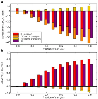
Fig. 3. (a) Atmospheric CO

2

change (∆CO

2

) and (b) ∆δ

13

C

atl

change (∆(∆δ

13

C

atl

)) due to

the transport of salt (S), dissolved inorganic carbon (DIC) and alkalinity (ALK), nutrients, and

dissolved organic carbon (DOC, too small too be visible, less than 1 ppm). In all simulations

the transport of salt is activated. In the “S transport” experiment only salt is transported, in

“DIC+ALK transport” salt, DIC and ALK are transported, in “Nutrients transport” salt and

nutri-ents are transported. “All” is the effect of the simultaneous transport of all variables. ∆CO

2

is

the difference between the modeled CO

2

and the standard modeled CO

2

(LGM std, CO

2

=296

ppm). ∆(∆δ

13

_C

atl

) is the difference between the modeled ∆δ

13

C

atl

and the standard modeled

∆δ

13

_C

atl

(LGM std).

27

Fig. 3. (a) Atmospheric CO₂ change (1CO₂) and (b) 1δ13C_atl change (1(1δ13Catl)) due to the transport of salt (S), dissolved

in-organic carbon (DIC) and alkalinity (ALK), nutrients, and dissolved organic carbon (DOC, too small too be visible, less than 1 ppm). In all simulations the transport of salt is activated. In the “S transport” experiment only salt is transported, in “DIC+ALK transport” salt, DIC and ALK are transported, in “Nutrients transport” salt and nu-trients are transported. “All” is the effect of the simultaneous trans-port of all variables. 1CO2is the difference between the modeled

CO2and the standard modeled CO2 (LGM std, CO2= 296 ppm). 1(1δ13Catl) is the difference between the modeled 1δ13Catl and

the standard modeled 1δ13Catl(LGM std).

oceanic circulation. The brines seem to be a good candidate as they will bring saline water to the abyss which will in-crease deep water salinity. In the following we will assess the impact of the brines and compare with data to either val-idate or reject such a possibility.

3.2 Atmospheric CO2drawdown induced by the

brine mechanism

The sinking of brines can have a very large effect on atmo-spheric carbon in our simulations (Fig. 2a). Atmoatmo-spheric CO2progressively decreases when the fraction of salt frac that sinks to the abyss increases. The frac = 0 simulation (no brine mechanism) corresponds to the standard LGM simula-tion (LGM-std), where CO2is 296 ppm. The maximum ef-fect of the brines is obtained for frac = 1, i.e. when all the salt released by sea ice formation sinks to the bottom of the ocean with the brine mechanism. The latter gives a maximum CO2 drop of about 52 ppm (CO2is 244 ppm). In this case it takes approximately 3000 years for the model to gain steady state

-60 -30 0 30 60 4000 3000 2000 1000 0 depth (m)

PI

a

-60 -30 0 30 60 4000 3000 2000 1000 0

LGM, frac=0

b

-60 -30 0 30 60 latitude (degree) 4000 3000 2000 1000 0 depth (m)

LGM, frac=0.5

c

-60 -30 0 30 60 latitude (degree) 4000 3000 2000 1000 0

LGM, frac=1

d

8 4 0 4 8 12 16 20 24

Fig. 4. Simulated meridional overturning stream function (Sv) in the Atlantic for (a) the

Pre-industrial (PI) simulation, (b) the standard LGM simulation (LGM-std) with f rac=0 (no impact of

brines), (c) the LGM simulation with f rac=0.5 (medium impact of brines), (d) the LGM

simula-tion with f rac=1 (maximum impact of brines).

28

Fig. 4. Simulated meridional overturning stream function (Sv) in the Atlantic for (a) the Pre-industrial (PI) simulation, (b) the standard LGM

simulation (LGM-std) with frac = 0 (no impact of brines), (c) the LGM simulation with frac = 0.5 (medium impact of brines), (d) the LGM simulation with frac = 1 (maximum impact of brines).

again after the onset of the sinking of brines, as the ocean circulation has to adapt to the induced change of density dis-tribution (Fig. 1b).

To understand the reasons of the atmospheric CO2 draw-down, we first assess which variable transport is a major con-tributor to these changes (Fig. 3a). We explore the impact of the sinking of salt alone, then we add either dissolved inor-ganic carbon (DIC) and alkalinity (ALK), nutrients (phos-phate and nitrate) or dissolved organic carbon (DOC). The transport of salt is activated in all simulations as it is the ini-tial reason for the sinking of the brines.

First we consider only the transport of salt to the deep ocean; the other variables do not sink with the brines. The salt sink accounts for the largest part of the CO2 drop (ap-proximately 60% of the CO2 drawdown due to the brine mechanism, Fig. 3a). The increased salinity of the bottom waters results in higher upper to deep ocean density differ-ence (Fig. 1b). Hdiffer-ence the deep stratification is enhanced and the oceanic circulation modified (Fig. 4). In the standard glacial simulation the atlantic meridional overturning circu-lation is slightly different from the pre-industrial one. The upper branch is shallower while the lower branch more in-tense and penetrates farther north (Fig. 4a and b). With the sinking of salt the vertical density gradient is higher. This leads to a more reduced upper branch while the lower branch expands upwards (Fig. 4c and d). The ventilation of the lower branch is reduced resulting in a decoupling between upper

and deep waters. The carbon enriched Antarctic Bottom Wa-ter (AABW) is less mixed with the surrounding waWa-ters and constitutes a greater volume of water. The trapping of CO2 released from the remineralization of organic matter in the deep ocean is then more efficient. The deep carbon reser-voir has thus expanded thanks to the change of circulation induced by the salt transport alone.

The transport of dissolved inorganic carbon (DIC) and al-kalinity (ALK) by brines also plays a role as it further de-creases atmospheric CO2 (Fig. 3). The direct transport of DIC and ALK to the abyss helps building an increased deep oceanic carbon reservoir as carbon is brought to the deep ocean but can not escape because of the stratification set by the increased density. In these sensitivity experiments, salt, DIC and ALK are transported. If only DIC and ALK were transported, the CO2change would be much greater, but with the salt transport the DIC and ALK concentrations in the sur-face are already depleted so that the effect of transporting DIC and ALK is not as effective.

The transport of nutrients has an opposite effect, as their transport to the abyss decreases their surface concentrations and thus the biological activity (Fig. 3). The biological pump being less efficient, less atmospheric CO2is taken up by the ocean. Yet this effect is smaller than the two previous ones. Additionaly the transport of DOC is negligible compared to the other mechanisms (less than 1 ppm).

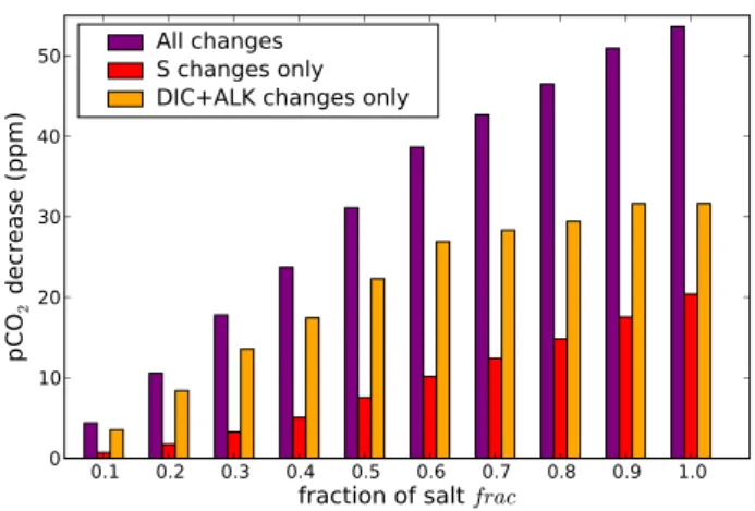
Now that we have seen that the salt sink is the main driver of the CO2drop and that the DIC and ALK transport can also play a role, we investigate how they impact the atmospheric CO2. Because of the direct effect of the salt sink (transport from the surface to the bottom) and indirect effect (change of oceanic circulation because of the stratification) the dis-tribution of salinity, DIC and ALK in the ocean is modified (especially the repartition between surface and deep waters). The changed surface concentrations modify the oceanic dis-solved CO2which ultimately drives atmospheric CO2.

Because of the salt transport by brines, salinity is increased in the deep ocean (Fig. 2c) and decreased in the surface. As the solubility of CO2 increases when salinity decreases it results in an atmospheric CO2 drawdown. To quantify this impact we have run the geochemical module of CLIMBER-2 alone forced by the standard distribution of all variables (from the LGM-std simulation without brines) except salin-ity. For the latter we prescribe the distribution obtained in the simulation with brines for frac = 0 to 1. This allows us to get the CO2change only due to the salinity distribution change. It appears that the modification of the salinity dis-tribution generally accounts for around 1/4 to a 1/3rd of the total CO2decrease (Fig. 5).

Similarly, DIC and ALK are increased in the deep ocean and decreased in the surface (Fig. 6), both because of the salt transport induced stratification (we have seen that this is the main process) and the direct transport of DIC and ALK by brines. To assess the impact of the change of DIC and ALK distribution we realize the same test as for salinity. With the geochemical module of CLIMBER-2 we evaluate the impact of the change of distribution of DIC and ALK alone for frac = 0 to 1. It shows that the DIC and ALK dis-tribution modification can generally explain between 1/2 and 2/3rd of the oceanic pCO2decrease (Fig. 5). Indeed, as the brines sink and make the deep ocean saltier, increased verti-cal stratification results. Southern convection (formation of Antarctic Bottom Water, AABW) is greatly reduced and very little exchange exists from the deep ocean to the surface, cre-ating a deep isolated water mass that is enriched in DIC and ALK (while the surface is depleted, Fig. 6). With respect to oceanic pCO2, DIC and ALK changes have opposite ef-fects (reduced surface DIC decreases pCO2, reduced ALK increases pCO2), but the DIC change prevails and results in a net oceanic pCO2decrease.

3.3 Impact of brines on oceanic δ13C

δ13C is usually used to track oceanic circulation, since their changes reflect the changes in ventilation of the different wa-ter masses (Duplessy et al., 1988; Curry and Oppo, 2005; K¨ohler and Bintanja, 2008). In the brine simulations, the modeled 1δ13Catl in the Atlantic Ocean is increased when the fraction of salt frac increases (Fig. 2b), which improves the results compared to proxy data. Several mechanisms can affect 1δ13Catl, as biology and circulation both impact the

0.1 0.2 0.3 0.4 0.5 0.6 0.7 0.8 0.9 1.0

fraction of salt

frac 0 10 20 30 40 50

pC

O

2

d

ec

re

as

e (

pp

m

)

All changes

S changes only

DIC+ALK changes only

Fig. 5. Mean global ocean surface pCO2decrease due to the brine mechanism as a function

of the fraction of salt rejected by sea ice formation used for the brine mechanism (fraction of salt f rac, 0 ≤ f rac ≤ 1). The pCO2is calculated from the chemical formulas of the surface

ocean where the geochemical fields (salinity, temperature, DIC and ALK) are imposed and taken from the simulations with CLIMBER-2. In the pCO2calculations (except “All changes”)

all the geochemical fields are from the standard LGM run (LGM-std, f rac=0) except for one variable. Hence the “S changes only” (red) is the pCO2change due to the contribution of the

modification in the salinity (S) distribution only (the distribution of the other variables is the one from the standard simulation). Similarly, the “DIC + ALK changes only” (orange) corresponds to the contribution of the modification of dissolved inorganic carbon (DIC) and alkalinity (ALK) only. However, “All Changes” (purple) corresponds to the decrease due to the change of distribution of all oceanic variables.

29

Fig. 5. Mean global ocean surface pCO₂decrease due to the brine mechanism as a function of the fraction of salt rejected by sea ice formation used for the brine mechanism (fraction of salt frac, 0 ≤ frac ≤ 1). The pCO2is calculated from the chemical formulas

of the surface ocean where the geochemical fields (salinity, temper-ature, DIC and ALK) are imposed and taken from the simulations with CLIMBER-2. In the pCO2calculations (except “All changes”)

all the geochemical fields are from the standard LGM run (LGM-std, frac = 0) except for one variable. Hence the “S changes only” (red) is the pCO₂change due to the contribution of the modification in the salinity (S) distribution only (the distribution of the other vari-ables is the one from the standard simulation). Similarly, the “DIC + ALK changes only” (orange) corresponds to the contribution of the modification of dissolved inorganic carbon (DIC) and alkalinity (ALK) only. However, “All Changes” (purple) corresponds to the decrease due to the change of distribution of all oceanic variables.

distribution of δ13C. Indeed, the vertical gradient of δ13C is primarily due the biological activity which preferentially incorporates 12C during photosynthesis. This tends to de-plete the upper waters of12C and hence increase δ13C. On the opposite, when organic matter is remineralized deeper in the ocean it releases12C thus decreases the deep δ13C. This process is then modulated by the oceanic circulation which transports and mixes water masses with different δ13C sig-natures and thus modifies the δ13C distribution. With the brine mechanism these two processes are involved as the salt transport alters circulation, the DIC, ALK and DOC trans-port directly modifies the upper and deep δ13C values, and the nutrients transport impacts the biological activity.

To assess the role of the salt, DIC and ALK, nutrients and DOC transport on the increase of 1δ13Catl we ana-lyze the same simulations as for CO2, when considering the transport of each of the variables (Fig. 3b). As for the CO2 decrease, the salt transport plays an important role. The 1δ13Catl increase is explained entirely by the salt transport. Because of the brine-induced stratification and resulting modified circulation (Fig. 4) the waters are less mixed. Hence the effect of the biological pump becomes

-60

-30

0

30

60

4000

3000

2000

1000

0

depth (m)

DIC

frac=0

a

-60

-30

0

30

60

4000

3000

2000

1000

0

depth (m)

frac=0.5

c

-60

-30

0

30

60

latitude (degree)

4000

3000

2000

1000

0

depth (m)

frac=1

d

-60

-30

0

30

60

4000

3000

2000

1000

0

frac=0

ALK

b

-60

-30

0

30

60

4000

3000

2000

1000

0

frac=0.5

d

-60

-30

0

30

60

latitude (degree)

4000

3000

2000

1000

0

frac=1

f

1900

2000

2100

2200

2300

2400

2500

Fig. 6. (a,c,d) Dissolved inorganic carbon (DIC) (µmol/kg) and (b,d,f) alkalinity (ALK) (µmol/kg)

distribution in the Atlantic for (a, b) the standard simulation (LGM-std) with f rac=0 (no impact of

brines), (c, d) f rac=0.5 (medium impact of brines), (e, f) f rac=1 (maximum impact of brines).

30

Fig. 6. (a), (c), (e) Dissolved inorganic carbon (DIC) (µmol/kg) and (b), (d), (f) alkalinity (ALK) (µmol/kg) distribution in the Atlantic for

(a), (b) the standard simulation (LGM-std) with frac = 0 (no impact of brines), (c), (d) frac = 0.5 (medium impact of brines), (e), (f) frac = 1 (maximum impact of brines).

more important compared to the mixing. The biological pump increases the vertical δ13C gradient. On the contrary the mixing lowers this gradient. Because the mixing is less intense the vertical gradient increases with lower deep δ13C and higher upper δ13C.

The DIC and ALK transport as well as nutrient transport have an opposite yet minor effect. The DIC and ALK trans-port brings high surface δ13C values down to the bottom and tends to lower the 1δ13Catl, but it has only a small impact of generally less than 0.1‰. The transport of nutrients lowers the surface nutrient concentration which decreases the bio-logical production. As the latter is responsible for the initial

1δ13Catlit also lowers 1δ13Catl. However this effect is neg-ligible (less than 0.1‰). Finally the effect of DOC transport is too small to be seen.

It appears that the salt transport is clearly the main pro-cess driving the 1δ13Catlincrease. On the contrary the other variables have only a small impact and tend to decrease

1δ13Catl. The 1δ13Catl is thus improved due to the change of circulation.

3.4 Amplifications by low vertical diffusion

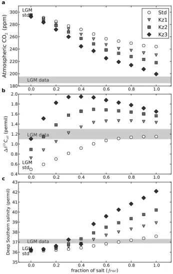
In the previous simulations, only the impact of brines on convection and advection was taken into account via salin-ity changes. But it is highly probable that such changes would also reduce vertical diffusion. CLIMBER-2 prescribes vertical diffusion as a fixed vertical profile, whereas in the-ory it depends on the vertical density profile in the ocean. The brine induced stratification would therefore also change

101 ₁₀2 Kz (10−4 cm2/s) 5000 4000 3000 2000 1000 0 Depth (m) Standard Kz0 Kz1 Kz2 Kz3

Fig. 7. Vertical diffusion coefficient profiles imposed in the simulations. Kz0 is the standard

profile, Kz1, 2 and 3 are the low diffusion profiles used to test the impact of deep low diffusion.

31

Fig. 7. Vertical diffusion coefficient profiles imposed in the

simula-tions. Kz0 is the standard profile, Kz1, 2 and 3 are the low diffusion profiles used to test the impact of deep low diffusion.

diffusion, as the more stratified the water becomes, the less vertical diffusion there would be (it requires more energy to mix well stratified water masses). To test this impact on CO2, we conduct a series of simulations with the brine mecha-nism where three low vertical diffusion profiles (Kz1, Kz2 and Kz3) are prescribed (Fig. 7). The impact of such low diffusion profiles alone in CLIMBER-2 has been previously studied (Bouttes et al., 2009) which showed that it helps rec-oncile the deep glacial δ13C though with a small impact on atmospheric CO2(10 ppm decrease only). Here we test these low diffusion profiles when the brine mechanism is activated in the model. We run a set of simulations by varying the frac value between 0 and 1 for the three diffusion profiles.

The effect of low diffusion alone, that was previously an-alyzed, resulted in a very small impact on atmospheric CO2, which is the case for the frac = 0 simulations. When com-bined with brines, the brine induced CO2decline is amplified and it leads to a further significant CO2decrease (Fig. 8a). It shows a clear amplification of the brine mechanism. Indeed, the low diffusion prevents even more the mixing between the carbon enriched bottom waters and the surface. Therefore it amplifies the trapping of carbon in the deep ocean and results in the supplementary simulated CO2drawdown.

The amplification also applies for δ13C, especially for

1δ13Catl which is increased (Fig. 8b). Indeed, when low diffusion is added, the deep δ13C becomes even more nega-tive. The deep (below −3000 m) ocean δ13C distribution thus compares far better with the data than in our standard simula-tion (LGM-std) where the values were too high (Figs. 9 and 10). The upper (above −2000 m) values are greater, resulting in the stronger upper to deep gradient. Hence δ13C strongly supports the brine mechanism amplified by low diffusion. Yet even though the Antarctic Bottom Water (AABW) ex-pands and the Glacial North Atlantic Deep Water (GNADW) shoals, the δ13C values are still not negative enough in the in-termediate south. This suggests that either GNADW should

0.0 0.2 0.4 0.6 0.8 1.0 180 200 220 240 260 280 300

At

m

os

ph

er

ic

CO

2

(p

pm

)

LGM data LGM std

a

Std

Kz1

Kz2

Kz3

0.0 0.2 0.4 0.6 0.8 1.0 0.4 0.6 0.8 1.0 1.2 1.4 1.6 1.8 2.0 ∆ δ 13C at l (p er m il) LGM data LGM std

b

0.0 0.2 0.4 0.6 0.8 1.0

fraction of salt (frac) 35 36 37 38 39 40 41 42 43

Deep Southern salinity (permil)

LGM data

LGM std

c

Fig. 8. (a) Atmospheric CO

2

concentration, (b) ∆δ

13

C

atl

(mean upper (-2000 m to 0 m) to

deep (-5000 m to -3000 m) gradient in the Atlantic) and (c) salinity in the deep Southern ocean

(Atlantic sector, 50 degrees South, 3626 m depth) as a function of the fraction of salt released

by sea ice formation used for the brine mechanism (fraction of salt f rac, 0 ≤ f rac ≤ 1) for

different vertical diffusion profiles. Kz0 (grey) is the standard profile, Kz1, 2 and 3 are the

tested low diffusion profiles (black). The Last Glacial Maximum (LGM) data are from Monnin et

al., 2001; Curry and Oppo, 2005; K ¨ohler and Bintanja, 2008; Adkins et al., 2002.

₃₂

Fig. 8. (a) Atmospheric CO2 concentration, (b) 1δ13Catl (mean

upper (−2000 m to 0 m) to deep (−5000 m to −3000 m) gradient in the Atlantic) and (c) salinity in the deep Southern ocean (Atlantic sector, 50 degrees South, 3626 m depth) as a function of the fraction of salt released by sea ice formation used for the brine mechanism (fraction of salt frac, 0 ≤ frac ≤ 1) for different vertical diffusion profiles. Kz0 (grey) is the standard profile, Kz1, 2 and 3 are the tested low diffusion profiles (black). The Last Glacial Maximum (LGM) data are from Monnin et al., 2001; Curry and Oppo, 2005; K¨ohler and Bintanja, 2008; Adkins et al., 2002.

be further reduced and confined to the northern Atlantic, or that another southern water mass existed at intermediate depths (e.g. a Glacial Antarctic Intermediate Water). 3.5 Impact of brines and low diffusion on oceanic 114C The oceanic distribution of 114C can be modified by two different processes with the brine mechanism. The change of oceanic circulation induced by the transport of salt to the deep ocean alters the mixing of water masses. The mixing is lowered which tends to increase the vertical gradient and

-60

-30

0

30

60

4000

3000

2000

1000

0

depth (m)

DATA

interpolation

a

-60

-30

0

30

60

4000

3000

2000

1000

0

depth (m)

frac=0

b

-60

-30

0

30

60

4000

3000

2000

1000

0

depth (m)

frac=0.5

d

-60

-30

0

30

60

latitude (degree)

4000

3000

2000

1000

0

depth (m)

frac=1

f

-60

-30

0

30

60

4000

3000

2000

1000

0

_{frac=0, Kz1}

c

-60

-30

0

30

60

4000

3000

2000

1000

0

_{frac=0.5, Kz1}

e

-60

-30

0

30

60

latitude (degree)

4000

3000

2000

1000

0

_{frac=1, Kz1}

g

1.0

0.6

0.2

0.2

0.6

1.0

1.4

Fig. 9. δ

13

C (‰) distribution in the Atlantic. The dots represent the LGM data (Curry and

Oppo, 2005; K ¨ohler and Bintanja, 2008). (a) Interpolation of the data. (b,c,d,e,f,g) Modelled

δ

13

C distribution: (b,d,f) with the standard diffusion profile Kz0 (Figure 7); (c, e, g) with the low

diffusion profile Kz1 (Figure 7). (b, c) f rac=0 (no impact of brines), (d,e) f rac=0.5 (medium

impact of brines), (f,g) f rac=1 (maximum impact of brines).

33

Fig. 9. δ13C (‰) distribution in the Atlantic. The dots represent the LGM data (Curry and Oppo, 2005; K¨ohler and Bintanja, 2008).

(a) Interpolation of the data. (b), (c), (d), (e), (f), (g) Modelled δ13C distribution: (b), (d), (f) with the standard diffusion profile Kz0 (Fig. 7); (c), (e), (g) with the low diffusion profile Kz1 (Fig. 7). (b), (c) frac = 0 (no impact of brines), (d), (e) frac = 0.5 (medium impact of brines), (f), (g) frac = 1 (maximum impact of brines).

lower δ14C in the deep ocean. On the opposite, the DI14C transport during the sinking of brines brings DIC with high 14_{C from the surface to the bottom. It then increases the deep}

114C values and lower the vertical gradient. The change of circulation is the prevailing effect and the deep 114C values become very low (Fig. 11a, c and d). Yet only with the very extreme and probably unrealistic frac value (frac=1) can the circulation capture the increased deep-water ages present in the data (Robinson et al., 2005; Skinner et al., 2010).

The low diffusion enhances the vertical gradient as the deep ocean becomes even more isolated. The deep 114C data values can then be reached with lower frac values. With very low diffusion profiles (Kz2 and 3, Fig. 12), the deep wa-ter 114C become too low showing that the diffusion should be lowered but not as much.

3.6 Glacial-interglacial carbon cycle changes

Previous studies with simple box models showed that a re-duced Southern ocean vertical mixing rate, which is im-posed in the model, can reduce atmospheric CO2 (Paillard

-60

-30

0

30

60

4000

3000

2000

1000

0

depth (m)

frac=0, Kz2

a

-60

-30

0

30

60

4000

3000

2000

1000

0

depth (m)

frac=0.5, Kz2

c

-60

-30

0

30

60

latitude (degree)

4000

3000

2000

1000

0

depth (m)

frac=1, Kz2

e

-60

-30

0

30

60

4000

3000

2000

1000

0

_{frac=0, Kz3}

b

-60

-30

0

30

60

4000

3000

2000

1000

0

_{frac=0.5, Kz3}

d

-60

-30

0

30

60

latitude (degree)

4000

3000

2000

1000

0

_{frac=1, Kz3}

f

1.0

0.6

0.2

0.2

0.6

1.0

1.4

Fig. 10. δ

13

C (‰) distribution in the Atlantic. The dots represent the LGM data (Curry and

Oppo, 2005; K ¨ohler and Bintanja, 2008). (a,b,c,d,e,f) Modelled δ

13

C distribution: (a, c, e) with

the low diffusion profile Kz2 (Figure 7); (b, d, f) with the low diffusion profile Kz3 (Figure 7).

(a, b) f rac=0 (no impact of brines), (c, d) f rac=0.5 (medium impact of brines), (e, f) f rac=1

(maximum impact of brines).

34

Fig. 10. δ13C (‰) distribution in the Atlantic. The dots represent the LGM data (Curry and Oppo, 2005; K¨ohler and Bintanja, 2008).

(a), (b), (c), (d), (e), (f) Modelled δ13C distribution: (a), (c), (e) with the low diffusion profile Kz2 (Fig. 7); (b), (d), (f) with the low diffusion profile Kz3 (Fig. 7). (a), (b) frac = 0 (no impact of brines), (c), (d) frac = 0.5 (medium impact of brines), (e), (f) frac = 1 (maximum impact of brines).

and Parrenin, 2004; K¨ohler et al., 2005). It also decreases the deep Southern δ13C (K¨ohler et al., 2005). More com-plex models of intermediate comcom-plexity and general circula-tion showed that changes in the oceanic circulacircula-tion impacts the δ13C distribution in the ocean. Reducing the strength of the meridional overturning circulation by adding fresh water fluxes to the North Atlantic tends to decrease the simulated

δ13C of the deep ocean in line with data (Tagliabue et al., 2009). Alternatively, imposing a lower vertical mixing by changing the vertical diffusion profile also increases the up-per to deep oceanic δ13C in agreement with data (Bouttes et al., 2009). However in both cases the associated at-mospheric CO2 drawdown remains small compared to the glacial-interglacial change (less than 10 ppm compared to

∼90 ppm).

With the sinking of brines, the necessary change of circu-lation which leads to an increase of the oceanic vertical δ13C gradient is simulated with a more physical mechanism (no

artificial fresh water flux is added). Moreover the CO2 draw-down simulated is much more significant. With the maxi-mum effect of the sinking of brines (frac = 1) the CO2 draw-down is 52 ppm. With less extreme values of frac around 0.5, the CO2 decrease is around 30 ppm, which can be further amplified by 5 to 15 ppm with vertical low diffusion. frac values around 0.5 are the most plausible values as they are both supported by the comparisons of model results with data and modern observations. Indeed, comparisons between the modelled salinity and 1δ13_{C with data are in better} agree-ment for frac values around 0.5 with the low diffusion profile Kz1 (Fig. 8), as well as 114C (Fig. 11). Such a frac value is also close to 0.62 which corresponds to the observed ∼62% of the salt flux rapidly released by sea ice formation that is released out of the fjord in the Norwegian Sea (Haarpaint-ner et al., 2001). Yet, though the simulated CO2 drop is important it is still not enough indicating the need for other processes.

-60

-30

0

30

60

4000

3000

2000

1000

0

depth (m)

frac=0

a

-60

-30

0

30

60

4000

3000

2000

1000

0

depth (m)

frac=0.5

c

-60

-30

0

30

60

latitude (degree)

4000

3000

2000

1000

0

depth (m)

frac=1

e

-60

-30

0

30

60

4000

3000

2000

1000

0

_{frac=0, Kz1}

b

-60

-30

0

30

60

4000

3000

2000

1000

0

_{frac=0.5, Kz1}

d

-60

-30

0

30

60

latitude (degree)

4000

3000

2000

1000

0

_{frac=1, Kz1}

f

350

300

250

200

150

100

50

Fig. 11. ∆

14

C (‰) distribution in the Atlantic simulated by the model (where ∆

14

C= 1000 ×

(

DI

_DIC

14

C

− 1)). The dots represent the LGM data (Robinson et al., 2005; Skinner et al., 2010).

(a, c, e) with the standard diffusion profile Kz0 (Figure 7); (b, d, f) with the low diffusion profile

Kz1 (Figure 7). (a, b) f rac=0 (no impact of brines), (c, d) f rac=0.5 (medium impact of brines),

(e, f) f rac=1 (maximum impact of brines).

35

Fig. 11. 114C (‰) distribution in the Atlantic simulated by the model (where 114C= 1000 · (DI_DIC14C−1)). The dots represent the LGM data (Robinson et al., 2005; Skinner et al., 2010). (a), (c), (e) with the standard diffusion profile Kz0 (Fig. 7); (b), (d), (f) with the low diffusion profile Kz1 (Fig. 7). (a), (b) frac = 0 (no impact of brines), (c), (d) frac = 0.5 (medium impact of brines), (e), (f) frac = 1 (maximum impact of brines).

Hence, although the brine mechanism has the potential to decrease significantly atmospheric CO2, additional mech-anisms are also very likely to be involved. In particu-lar, within the already tested mechanisms, the addition of carbonate compensation is a likely candidate, since it would further decrease CO2by around 30 ppm (Broecker and Peng, 1987; Brovkin et al., 2007). Additionally, modifications to the biological pump (linked to dust reconstructions and phytoplankton stoichiometry) can provide an additional 10– 25 ppm (Bopp et al., 2003; Tagliabue et al., 2009), as well as increasing carbon export in line with proxy reconstruc-tions. Overall, a combination of low diffusion, carbonate compensation and enhanced biological pump added to the brine mechanism could yield the full range of glacial to in-terglacial variability of CO2.

4 Conclusions

In conclusion, the brine mechanism can lead to a large atmo-spheric CO2 drop supported by the concomitant simulated changes in oceanic carbon isotope distribution, in agreement with proxy data. We have shown that this CO2decline is pri-marily due to the salt transport although the DIC and ALK sink also play a role. Because of the salt transport to the deep ocean the oceanic circulation is modified and the deep ocean becomes more stratified and decoupled from the surface. The abyss is enriched in carbon which is trapped because of the reduced mixing with other water masses. This decrease can be amplified if the simultaneous impact on oceanic vertical diffusion is accounted for. The low diffusion would further reduce the mixing between the deep and upper ocean, hence

-60

-30

0

30

60

4000

3000

2000

1000

0

depth (m)

frac=0, Kz2

a

-60

-30

0

30

60

4000

3000

2000

1000

0

depth (m)

frac=0.5, Kz2

c

-60

-30

0

30

60

latitude (degree)

4000

3000

2000

1000

0

depth (m)

frac=1, Kz2

e

-60

-30

0

30

60

4000

3000

2000

1000

0

_{frac=0, Kz3}

b

-60

-30

0

30

60

4000

3000

2000

1000

0

_{frac=0.5, Kz3}

d

-60

-30

0

30

60

latitude (degree)

4000

3000

2000

1000

0

_{frac=1, Kz3}

f

350

300

250

200

150

100

50

Fig. 12. ∆

14

C (‰) distribution in the Atlantic simulated by the model (where ∆

14

C= 1000 ×

(

DI

_DIC

14

C

− 1)). The dots represent the LGM data (Robinson et al., 2005; Skinner et al., 2010).

(a, c, e) with the low diffusion profile Kz2 (Figure 7); (b, d, f) with the low diffusion profile Kz3

(Figure 7). (a, b) f rac=0 (no impact of brines), (c, d) f rac=0.5 (medium impact of brines), (e, f)

f rac=1 (maximum impact of brines).

36

Fig. 12. 114C (‰) distribution in the Atlantic simulated by the model (where 114C= 1000 · (DI_DIC14C−1)). The dots represent the LGM data (Robinson et al., 2005; Skinner et al., 2010). (a), (c), (e) with the low diffusion profile Kz2 (Fig. 7); (b), (d), (f) with the low diffusion profile Kz3 (Fig. 7). (a), (b) frac = 0 (no impact of brines), (c), (d) frac = 0.5 (medium impact of brines), (e), (f) frac = 1 (maximum impact of brines).

decreasing atmospheric CO2and increasing the 1δ13Catl in line with data. We hypothesize that a combination of the al-ready known carbonate compensation mechanism, iron fer-tilization, brine mechanism and low diffusion would be suf-ficient to reach the glacial value of 190 ppm. The brine mech-anism provides two major features: a physical way of setting the needed glacial deep ocean stratification and a direct con-nection from surface to deep waters, which is crucial to cre-ate a very large deep ocean carbon reservoir. Beyond the un-derstanding of past climate, this mechanism sheds new light on ocean dynamics. Brines have a crucial role in the forma-tion of deep water and should therefore be better accounted for in climate models.

Acknowledgements. We thank Alessandro Tagliabue for comments

and ideas, and Laurent Bopp for discussion. We also thank Bill Curry and Peter K¨ohler for providing the δ13C data and Victor Brovkin for his help on the CLIMBER-2 model. We are greatful to Elisabeth Michel for her help with 114C, and to two anonymous reviewers and Gerald Ganssen for their comments which helped improve this manuscript.

Edited by: G. M. Ganssen

References

Adkins, J. F., McIntyre, K., and Schrag, D. P.: The salinity, temper-ature, and δ18O of the glacial deep ocean, Science, 298, 1769– 1773, 2002.

Archer, D. and Maier-Reimer, E.: Effect of deep-sea sedimentary calcite preservation on atmospheric CO2concentration, Nature,

367, 260–263, doi:10.1038/367260a0, 1994.

Archer, D., Winguth, A., Lea, D., and Mahowald, N.: What caused the glacial/interglacial pCO2cycles?, Rev. Geophys., 38, 159–

189, 2000.

Archer, D. E., Martin, P. A., Milovich, J., Brovkin, V., Plattner, G.-K., and Ashendel, C.: Model sensitivity in the effect of Antarctic sea ice and stratification on atmospheric pCO2,

Paleo-ceanography, 18(1), 1012, doi:10.1029/2002PA000760, 2003. Berger, A. L.: Long-term variations of daily insolation and

Quater-nary climatic changes, J. Atmos. Sci., 35, 2362–2368, 1978. Berger, W. H.: Increase of carbon dioxide in the atmosphere during

Deglaciation: the coral reef hypothesis, Naturwissenschaften, 69, 87–88, 1982.

Bird, M. I., Lloyd, J., and Farquhar, G. D.: Terrestrial carbon stor-age at the LGM, Nature, 371, 566, 1994.

Bopp, L., Kohfeld, K. E., Qu´er´e, C. L., and Aumont, O.: Dust impact on marine biota and atmospheric CO2 during

glacial periods, Paleoceanography, 18(2), 1046, doi:10.1029/ 2002PA000810, 2003.

Bouttes, N., Roche, D. M., and Paillard, D.: Impact of strong deep ocean stratification on the carbon cycle, Paleoceanography, 24, PA3203, doi:10.1029/2008PA001707, 2009.

Broecker, W. S. and Peng, T.-H., eds.: Tracers in the Sea, Lamont-Doherty Geological Observatory of Columbia University, Pal-isades, New York, USA, 466–484, 1982.

Broecker, W. S. and Peng, T.-H.: The Role of CaCO3

Compen-sation in the Glacial to Interglacial Atmospheric CO₂Change, Global Biogeochem. Cy., 1(1), 15–29, 1987.

Brovkin, V., Hofmann, M., Bendtsen, J., and Ganopolski, A.: Ocean biology could control atmospheric δ13C during glacial-interglacial cycle, Geochem. Geophys. Geosyst., 3(5), 1027, doi: 10.1029/2001GC000270, 2002.

Brovkin, V., Bendtsen, J., Claussen, M., Ganopolski, A., Kubatzki, C., Petoukhov, V., and Andreev, A.: Carbon cycle, vegetation, and climate dynamics in the Holocene: Experiments with the CLIMBER-2 model, Global Biogeochem. Cy., 16(4), 1139, doi: 10.1029/2001GB001662, 2002a.

Brovkin, V., Ganopolski, A., Archer, D., and Rahmstorf, S.: Lower-ing of glacial atmospheric CO2in response to changes in oceanic

circulation and marine biogeochemistry, Paleoceanography, 22, PA4202, doi:10.1029/2006PA001380, 2007.

Crowley, T.: Ice Age Terrestrial Carbon Changes Revisited, Global Biogeochem. Cy., 9(3), 377–389, 1995.

Curry, W. B. and Oppo, D. W.: Glacial water mass geometry and the distribution of δ13C of 6CO₂in the western Atlantic Ocean, Paleoceanography, 20, PA1017, doi:10.1029/2004PA001021, 2005.

Duplessy, J.-C., Shackleton, N., Fairbanks, R., Labeyrie, L., Oppo, D., and Kallel, N.: Deep water source variations during the last climatic cycle and their impact on the global deepwater circula-tion, Paleoceanography, 3, 343–360, 1988.

Foldvik, A., Gammelsrød, T., Østerhus, S., Fahrbach, E., Rohardt, G., Schr¨oder, M., Nicholls, K. W., Padman, L., and Woodgate,

R. A.: Ice shelf water overflow and bottom water formation in the southern Weddell Sea, J. Geophys. Res., 109, C02 015, doi: 10.1029/2003JC002008, 2004.

Foster, T. D. and Carmack, E.: Temperature and salinity structure in the Weddell Sea, J. Phys. Oceanogr., 6, 36–44, 1976. Ganopolski, A., Petoukhov, V., Rahmstorf, S., Brovkin, V.,

Claussen, M., Eliseev, A., and Kubatzki, C.: CLIMBER-2: A climate system model of intermediate complexity, part II: Model sensitivity, Clim. Dyn., 17, 735–751, 2001a.

Gersonde, R., Crosta, X., Abelmann, A., et al.: Sea-surface temper-ature and sea ice distribution of the Southern Ocean at the EPI-LOG Last Glacial Maximum – A circum-Antarctic view based on siliceous microfossil records, Quat. Sci. Rev., 24, 869–896, 2005.

Haarpaintner, J., Gascard, J. C., and Haugan, P. M.: Ice production and brine formation in Storfjorden, Svalbard, J. Geophys. Res, 106, 14001–14013, 2001.

Jahn, A., Claussen, M., Ganopolski, A., and Brovkin, V.: Quantify-ing the effect of vegetation dynamics on the climate of the Last Glacial Maximum, Clim. Past, 1, 1–7, doi:10.5194/cp-1-1-2005, 2005.

Joughin, I. and Padman, L.: Melting and freezing beneath Filchner-Ronne Ice Shelf, Antarctica, Geophys. Res. Lett., 30, 1477, doi: 10.1029/2003GL016941, 2003.

Kikuchi, T., Wakatsuchi, M., and Ikeda, M.: A numerical investiga-tion of the transport process of dense shelf water from a conti-nental shelf to a slope, J. Geophys. Res., 104(C1), 1197–1210, 1999.

Kohfeld, K. E., Qu´er´e, C. L., Harrison, S. P., and Anderson, R. F.: Role of Marine Biology in Glacial-Interglacial CO2Cycles,

Sci-ence, 308, 74–78, 2005.

K¨ohler, P. and Bintanja, R.: The carbon cycle during the Mid Pleis-tocene Transition: the Southern Ocean Decoupling Hypothesis, Clim. Past, 4, 311–332, doi:10.5194/cp-4-311-2008, 2008. K¨ohler, P., Fischer, H., Munhoven, G., and Zeebe, R. E.:

Quanti-tative interpretation of atmospheric carbon records over the last glacial termination, Global Biogeochem. Cy., 19, GB4020, doi: 10.1029/2004GB002345, 2005a.

K¨ohler, P., Fischer, H., and Schmitt, J.: Atmospheric δ13CO2

and its relation to pCO2 and deep ocean δ13C during the

late Pleistocene, Paleoceanography, 25, PA1213, doi:10.1029/ 2008PA001703, 2010.

Luthi, D., Floch, M. L., Bereiter, B., Blunier, T., Barnola, J.-M., Siegenthaler, U., Raynaud, D., Jouzel, J., Fischer, H., Kawamura, K., and Stocker, T. F.: High-resolution carbon dioxide concentra-tion record 650,000-800,000 years before present, Nature, 453, 379–382, doi:10.1038/nature06949, 2008.

MARGO Project Members: Constraints on the magnitude and patterns of ocean cooling at the Last Glacial Maximum, Nat. Geosci., 2, 127–132, doi:10.1038/ngeo411, 2009.

Martin, J. H.: Glacial-Interglacial CO₂change: the iron hypothesis, Paleoceanography, 5, 1–13, 1990.

Matsumoto, K., Sarmiento, J. L., and Brzezinski, M. A.: Silicic acid leakage from the Southern Ocean: A possible explanation for glacial atmospheric pCO2, Global Biogeochem. Cy. , 16(3),

1031, doi:10.1029/2001GB001442, 2002.

Menviel, L., Timmermann, A., Mouchet, A., and Timm, O.: Meridional reorganizations of marine and terrestrial productiv-ity during Heinrich events, Paleoceanography, 23, PA1203, doi:

10.1029/2007PA001445, 2008b.

Monnin, E., Inderm¨uhle, A., Daellenbach, A., Flueckiger, J., Stauf-fer, B., Stocker, T. F., Raynaud, D., and Barnola, J.-M.: Atmo-spheric CO2Concentrations over the Last Glacial Termination,

Science, 291, 112–114, 2001.

Nicholls, K. W., Østerhus, S., Makinson, K., Gammelsrød, T., and Fahrbach, E.: Ice-ocean processes over the continental shelf of the southern Weddell Sea, Antarctica: A review, Rev. Geophys., 47, RG3003, doi:10.1029/2007RG000250, 2009.

Opdyke, B. N. and Walker, J. C. G.: Return of the coral reef hy-pothesis: Basin to shelf partitioning of CaCO3and its effect on

atmospheric CO₂, Geology, 20, 733–736, 1992.

Paillard, D. and Parrenin, F.: The Antarctic ice sheet and the trig-gering of deglaciations, Earth Planet. Sc. Lett., 227, 263–271, 2004.

Peltier, W. R.: Global glacial isostasy and the surface of the ice-age Earth: The ICE-5G (VM2) Model and GRACE, Annu. Rev. Earth Planet. Sci., 32, 111–49, doi:10.1146/annurev.earth.32. 082503.144359, 2004.

Petoukhov, V., Ganopolski, A., Eliseev, A., Kubatzki, C., and Rahmstorf, S.: CLIMBER-2: A climate system model of inter-mediate complexity, part I: Model description and performance for present climate, Clim. Dynam., 16, 1–17, 2000.

Ritz, C., Rommelaere, V., and Dumas, C.: Modeling the evolution of Antarctic ice sheet over the last 420,000 years: Implications for altitude changes in the Vostok region, J. Geophys. Res., 106, 31,943–31,964, 2001.

Robinson, L. F., Adkins, J. F., Keigwin, L. D., Southon, J., Fernan-dez, D. P., Wang, S.-L., , and Scheirer, D. S.: Radiocarbon Vari-ability in the Western North Atlantic During the Last Deglacia-tion, Science, 310, 1469–1473, doi:10.1126/science.1114832, 2005.

Rysgaard, S., Glud, R. N., Sejr, M. K., Bendtsen, J., and Chris-tensen, P. B.: Inorganic carbon transport during sea ice growth and decay: A carbon pump in polar seas, Geophys. Res., 112, C03 016, doi:10.1029/2006JC003572, 2007.

Rysgaard, S., Bendtsen, J., Pedersen, L. T., Ramløv, H., and Glud, R. N.: Increased CO2uptake due to sea ice growth and

decay in the Nordic Seas, J. Geophys. Res., 114, 114, doi: 10.1029/2008JC005088, 2009.

Shcherbina, A. Y., Talley, L. D., and Rudnick, D. L.: Direct Ob-servations of North Pacific Ventilation: Brine Rejection in the Okhotsk Sea, Science, 302, 1952–1955, doi:10.1126/science. 1088692, 2003.

Skinner, L. C., Fallon, S., Waelbroeck, C., Michel, E., and Barker, S.: Ventilation of the Deep Southern Ocean and Deglacial CO₂ Rise, Science, 328(5982), 1147–1151, doi:10.1126/science.1183627, 2010.

Skogseth, R., Haugan, P. M., and Haarpaintner, J.: Ice and brine production in Storfjorden from four winters of satellite and in situ observations and modeling, J. Geophys. Res., 109, C10 008, doi:10.1029/2004JC002384, 2004.

Skogseth, R., Smedsrud, L. H., Nilsen, F., and Fer, I.: Observa-tions of hydrography and downflow of brine-enriched shelf wa-ter in the Storfjorden polynya, Svalbard, J. Geophys. Res., 113, C08 049, doi:10.1029/2007JC004452, 2008.

Stephens, B. B. and Keeling, R. F.: The influence of Antarctic sea ice on glacial-interglacial CO2variations, Nature, 404, 171–174,

2000.

Tagliabue, A., Bopp, L., Roche, D. M., Bouttes, N., Dutay, J.-C., Alkama, R., Kageyama, M., Michel, E., and Paillard, D.: Quanti-fying the roles of ocean circulation and biogeochemistry in gov-erning ocean carbon-13 and atmospheric carbon dioxide at the last glacial maximum, Clim. Past, 5, 695–706, doi:10.5194/cp-5-695-2009, 2009.

Toggweiler, J. and Samuels, B.: Effect of Sea Ice on the Salinity of Antarctic Bottom Waters, J. Phys. Oceanogr., 25, 1980–1997, 1995.

Toggweiler, J. R.: Variation of atmospheric CO2by ventilation of

the ocean’s deepest water, Paleoceanography, 14(5), 571–588, 1999.

Toggweiler, J. R., Russell, J. L., and Carson, S. R.: Midlat-itude westerlies, atmospheric CO2, and climate change

dur-ing the ice ages, Paleoceanography, 21, PA2005, doi:10.1029/ 2005PA001154, 2006.

Wakatsuchi, M. and Ono, N.: Measurements of Salinity and Vol-ume of Brine Excluded From Growing Sea Ice, J. Geophys. Res., 88(C5), 2943–2951, 1983.

Watson, A. J. and Garabato, A. C. N.: The role of Southern Ocean mixing and upwelling in glacial-interglacial atmospheric CO2

change, Tellus B, 58(1), 73–87, doi:10.1111/j.1600-0889.2005. 00167.x, 2005.

Whitworth, T. and Nowlin, W.: Water Masses and currents of the Southern Ocean, J. Geophys. Res., 92, 6463–6476, 1987.