HAL Id: cea-02421745
https://hal-cea.archives-ouvertes.fr/cea-02421745
Submitted on 18 Mar 2020
HAL is a multi-disciplinary open access
archive for the deposit and dissemination of sci-entific research documents, whether they are pub-lished or not. The documents may come from teaching and research institutions in France or abroad, or from public or private research centers.
L’archive ouverte pluridisciplinaire HAL, est destinée au dépôt et à la diffusion de documents scientifiques de niveau recherche, publiés ou non, émanant des établissements d’enseignement et de recherche français ou étrangers, des laboratoires publics ou privés.
Neutron multiplication in random media: Reactivity
and kinetics parameters
Coline Larmier, Andrea Zoia, Fausto Malvagi, Eric Dumonteil, Alain Mazzolo
To cite this version:
Coline Larmier, Andrea Zoia, Fausto Malvagi, Eric Dumonteil, Alain Mazzolo. Neutron multiplication in random media: Reactivity and kinetics parameters. Annals of Nuclear Energy, Elsevier Masson, 2017, 111, pp.391-406. �10.1016/j.anucene.2017.09.006�. �cea-02421745�
Neutron multiplication in random media: reactivity and
kinetics parameters
Coline Larmiera, Andrea Zoiaa,∗, Fausto Malvagia, Eric Dumonteilb, Alain Mazzoloa
aDEN-Service d’´etudes des r´eacteurs et de math´ematiques appliqu´ees (SERMA), CEA,
Universit´e Paris-Saclay, F-91191, Gif-sur-Yvette, France
bIRSN, 31 Avenue de la Division Leclerc, 92260 Fontenay aux Roses, France.
Abstract
Eigenvalue problems for neutron transport in random geometries are key for many applications, ranging from reactor design to criticality safety. In this work we examine the behaviour of the reactivity and of the kinetics parame-ters (the effective delayed neutron fraction and the effective neutron generation time) for three-dimensional UOX and MOX assembly configurations where a portion of the fuel pins has been randomly fragmented by using various mixing statistics. For this purpose, we have selected stochastic tessellations of the Pois-son, Voronoi and Box type, which provide convenient models for the random partitioning of space, and we have generated an ensemble of assembly realiza-tions; for each geometry realization, criticality calculations have been performed by using the Monte Carlo code TRIPOLI-4 R, developed at CEA. We have then examined the evolution of the ensemble-averaged observables of interest as a function of the average chord length of the random geometries, which is roughly proportional to the correlation length of the fuel fragmentation. The method-ology proposed in this work is fairly general and could be applied, e.g., to the assessment of re-criticality probability following severe accidents.
Keywords: Random media, Monte Carlo, TRIPOLI-4 R, Kinetics parameters, Markov tessellations, Poisson, Voronoi.
∗Corresponding author
1. Introduction
Neutron multiplication in stochastic media has attracted intense research ef-forts, in view of many relevant applications emerging in reactor physics and criti-cality safety, such as the design of prismatic and pebble-bed reactors with double heterogeneity fuel (Murata et al., 1996;Liang et al., 2013; Brown and Martin,
5
2004), the analysis of neutron absorbers with dispersed poison grains (Doub,
1961) or MOX fuels with Pu-rich agglomerates (Yamamoto, 2010), optimal ra-dioactive waste storage (Williams,2003), and the assessment of the safety mar-gins due to the multiplication factor distribution (Pomraning, 1999; Williams,
2000;Williams and Larsen,2001), only to name a few.
10
The formal approach to these problems consists in averaging the critical Boltzmann equation with respect to the random configurations, and then solv-ing the correspondsolv-ing eigenvalue problem (Pomraning,1991,1999). Theoretical progress on such topics is hindered by the great amount of ingenuity required to derive exact results, even in the simplest models and configurations (Pomraning,
15
1999; Williams, 2000, 2003; Williams and Larsen, 2001). Perturbation theory can be helpful, but several simplifications are usually required, including mono-energetic transport, isotropic scattering, or diffusion approximation (Pomraning,
1999;Williams and Larsen,2001).
In this respect, Monte Carlo simulation offers a convenient tool for the
nu-20
merical analysis of eigenvalue problems in stochastic media. For this purpose, two complementary strategies have been proposed (Pomraning, 1991): the for-mer consists in generating by Monte Carlo methods a collection of realizations of random media (obeying some given distribution, which is supposed to accu-rately model the system under analysis) and then solving the eigenvalue problem
25
for each realization by using a transport code. The ensemble averages will finally yield the moments, and in principle also the full distribution, of the physical ob-servables of interest, e.g., the multiplication factor or the neutron flux shape. Such reference solutions are exact, since the stochastic nature of the medium is entirely preserved, including the effects on neutron trajectories possibly induced
30
by the spatial correlations. The latter consists in developing effective trans-port kernels capable of reproducing on-the-fly the ‘average’ behaviour of neu-tron displacement accounting for the underlying random heterogeneities, such as in the case of the well-known Chord Length Sampling algorithm (Zimmerman,
1990; Zimmerman and Adams, 1991; Donovan and Danon, 2003; Donovan et
35
al.,2003). In this case, a single eigenvalue calculation with effective jump distri-bution is sufficient, at the expense of sacrificing the correlations (whose effects must be typically neglected in constructing these algorithms).
Reference solutions, although computationally expensive, are nonetheless of utmost importance for the validation of approximate, albeit much faster
meth-40
ods, and for the verification of exact formulas (Levermore et al., 1986; Adams
et al.,1989;Malvagi et al.,1992;Su and Pomraning,1995;Zuchuat et al.,1994;
Larsen and Vasques, 2011; Brantley, 2011; Donovan and Danon, 2003;
Dono-van et al., 2003; Brantley and Palmer, 2009; Brantley, 2009). Significant ad-vances have been made in the numerical simulation of eigenvalue problems in
45
the presence of stochastic inclusions, where objects (typically spheres) are ran-domly placed within a background matrix (Murata et al., 1996; Liang et al.,
2013;Brown and Martin,2004). Stochastic inclusions emerge for instance in the modelling of the double heterogeneities in prismatic or pebble-bed reactors. In particular, highly sophisticated algorithms have been devised in order to properly
50
take into account boundary effects due to spheres not entirely contained in the medium (Grieshiemer et al.,2010;Ji and Martin.,2013). Eigenvalue calculations in stochastic tessellations, where the medium is supposed to be partitioned into a collection of random (fissile and non-fissile) volumes obeying a given mixing statistics (Pomraning,1991), have been limited so far to one-dimensional
config-55
urations of the rod or slab type (Pomraning, 1999;Williams and Larsen,2001). Such models might represent, e.g., the accidental positioning of fuel lumps into moderating material, in the context of criticality safety.
In a series of recent papers, we have examined the statistical properties of linear particle transport through d-dimensional stochastic tessellations without
60
multiplication (Lepage et al., 2011; Larmier et al., 2017a). In particular, we have computed reference solutions for the ensemble-averaged scalar flux and the reflection and transmission probabilities for Poisson (Markov) mixing statistics by revisiting the benchmark originally proposed by Adam, Larsen and Pomran-ing (Adams et al., 1989;Brantley, 2011;Brantley and Palmer, 2009;Brantley,
65
2009), and we have then extended our findings to the case of Voronoi and Box statistics (Larmier et al.,2017b).
In this work, we will adopt stochastic tessellations (Santalo,1976;Torquato,
2013) in order to assess the impact of the three-dimensional random fragmen-tation of fuel elements on the key safety parameters for criticality calculations,
70
including the multiplication factor keff, the effective delayed neutron fraction βeff,
and the effective neutron generation time `eff. In-pile fuel degradation might result from partial core melt-down during severe accidents, with melting, re-solidification and relocation (Hagen and Hofmann, 1987; Hofmann, 1999), as occurred in the case of the Three Mile Island unit 2 (Broughton et al., 1989).
75
evaluation of the re-criticality probability. To our best knowledge, the influence of random geometries on kinetics parameters has never been addressed before. Starting from a reference UOX or MOX assembly with 17 × 17 fuel pins, we will consider three perturbed configurations having the central pin, 7 × 7 central pins
80
and the whole 17 × 17 pins being randomly fragmented. We will assume that the random re-arrangement after melt-down can be described by ternary mix-ing statistics (Pomraning, 1991), accounting for the dispersion of the fuel, the cladding and the moderator, the average linear size of the chunks for each mate-rial being a free parameter of the model. For each realization, we will perform
85
criticality calculations by using the Monte Carlo transport code TRIPOLI-4 R developed at CEA (Brun et al.,2015), so as to investigate the distribution of keff,
βeffand `effas a function of the model parameters, including the material
compo-sitions, the kind of stochastic tessellation, the linear size of the random chunks, and the number of fragmented fuel pins.
90
In order to better grasp the physical behaviour of these systems without being hindered by the complexity of all the ingredients involved in nuclear accidents, the analysis of assembly configurations that will be carried out in this work is ad-mittedly highly simplified with respect to the realistic description of fuel degra-dation: for instance, we will focus exclusively on neutron transport, and we will
95
not include the effects due to thermal-hydraulics, thermo-mechanics or the com-plex physical-chemical reactions occurring in accidental transients (Hagen and
Hofmann, 1987; Hofmann, 1999). Nonetheless, the methodology proposed in this paper is fairly broad and can be applied without any particular restrictions to more sophisticated models.
100
This paper is organized as follows: in Sec. 2 we will briefly introduce the stochastic tessellations that will be used in this work. Then, in Sec. 3 we will describe the benchmark model for the partially melted fuel assembly. Simulation results for the multiplication factor and the kinetics parameters will be presented and discussed in Sec.4. Conclusions will be finally drawn in Sec.5.
105
2. Stochastic tessellations
Stochastic tessellations form a convenient class of probabilistic models to partition a given d-dimensional domain into random polyhedral cells (Santalo,
1976; Chiu et al., 2013; Torquato, 2013), and as such have been adopted in a broad spectrum of applications, ranging from material science (Gilbert, 1962;
110
Meijering, 1953) to stereology (Serra, 1982; Santalo, 1976): for an extensive review, see, e.g., (Santalo, 1976;Miles, 1972; Torquato, 2013). In this section, we introduce the three mixing statistics that will be used in order to generate the
random geometries for the criticality calculations. In particular, we will recall the algorithms for their construction based on Monte Carlo methods, and their main
115
statistical features. These algorithms have already been discussed elsewhere, but they are reported here in order for the paper to be self-contained. For the sake of conciseness, the three stochastic tessellations will be distinguished by their label m, namely, m =P for Poisson tessellations, m = V for Voronoi tessellations, and m =B for Box tessellations. The algorithms described in the following have
120
been implemented into a computer code that can perform the statistical analysis of an ensemble of realizations, and can produce input files for the TRIPOLI-4 R
Monte Carlo transport code (Brun et al.,2015). 2.1. Isotropic Poisson tessellations
Markovian mixing is generated by using isotropic Poisson geometries, which
125
form a prototype process of stochastic tessellations: a domain included in a d-dimensional space is partitioned by randomly generated (d − 1)-dimensional hyper-planes drawn from an underlying Poisson process (Santalo, 1976;Miles,
1970, 1972). An algorithm has been recently proposed for finite d-dimensional geometries (Serra,1982;Ambos and Mikhailov,2011), allowing for the explicit
130
construction of three-dimensional homogeneous and isotropic Poisson tessella-tions. In the following we will present the algorithm for the construction of these geometries restricted to a cubic box (further details are provided in (Larmier et
al.,2016)).
The algorithm starts by sampling a random number of hyper-planes NH from
a Poisson distribution of intensity 4ρPR, where R is the radius of the sphere circumscribed to the cube and ρP is the (arbitrary) density of the tessellation, carrying the units of an inverse length. This normalization of the density ρP cor-responds to the convention used in (Santalo, 1976), and is such that ρP yields the mean number of (d − 1)-hyperplanes intersected by an arbitrary segment of unit length. Then, we generate the planes that will cut the cube. We choose a ra-dius r uniformly in the interval [0, R] and then sample two additional parameters, namely, ξ1 and ξ2, from two independent uniform distributions in the interval
[0, 1]. A unit vector n = (n1, n2, n3)T with components
n1= 1 − 2ξ1 n2= q 1 − n21cos (2πξ2) n3= q 1 − n21sin (2πξ2)
is generated. Denoting by M the point such that OM = rn, the random plane will
135
By construction, this plane does intersect the circumscribed sphere of radius R but not necessarily the cube. The procedure is iterated until NH random planes
have been generated. The polyhedra defined by the intersection of such random planes are convex.
140
2.2. Poisson-Voronoi tessellations
Voronoi tessellations refer to another prototype process for isotropic random division of space (Santalo,1976). A portion of a space is decomposed into poly-hedral cells by a partitioning process based on a set of random points, called ‘seeds’. From this set of seeds, the Voronoi decomposition is obtained by
ap-145
plying the following deterministic procedure: each seed is associated with a Voronoi cell, defined as the set of points which are nearer to this seed than to any other seed. Such a cell is convex, because obtained from the intersection of half-spaces.
In this paper, we will exclusively focus on Poisson-Voronoi tessellations,
150
which form a subclass of Voronoi geometries (Meijering, 1953;Gilbert, 1962;
Miles,1972). The specificity of Poisson-Voronoi tessellations concerns the sam-pling of the seeds. In order to construct Poisson-Voronoi tessellations restricted to a cubic box of side L, we adopt the algorithm proposed in (Miles,1972). First, we choose the random number of seeds NSfrom a Poisson distribution of
param-155
eter (ρVL)3, where ρV characterizes the density of the tessellation. Then, NS
seeds are uniformly sampled in the box [−L/2, L/2]3. For each seed, we com-pute the corresponding Voronoi cell as the intersection of half-spaces bounded by the mid-planes between the selected seed and any other seed. In order to avoid confusion with the Poisson tessellations described above, we will mostly refer to
160
Poisson-Voronoi geometries simply as Voronoi tessellations in the following. 2.3. Poisson Box tessellations
Box tessellations form a class of anisotropic stochastic geometries, composed of rectangular boxes with random sides. For the special case of Poisson Box tes-sellations (as proposed by (Miles,1972)), a domain is partitioned by i) randomly
165
generated planes orthogonal to the x-axis, through a Poisson process of intensity ρx; ii) randomly generated planes orthogonal to the y-axis, through a Poisson
process of intensity ρy; iii) randomly generated planes orthogonal to the z-axis,
through a Poisson process of intensity ρz. In the following, we will assume that
the three parameters are equal, namely, ρx= ρy= ρz= ρB.
170
In order to tessellate a cube of side L, the construction algorithm is the
fol-lowing: we begin by sampling a random number Nx from a Poisson
distribu-tion of intensity ρBL. Then, we sample Nx points uniformly on the segment
[−L/2, L/2]. For each point of this set, we cut the geometry with the plane or-thogonal to the x-axis and passing through this point. We repeat this process for
175
the y-axis and the z-axis. For the sake of conciseness, we will denote by Box tessellations these Poisson Box tessellations. Poisson-Box tessellations have the remarkable property that their chord length distribution is almost identical to that of the homogeneous and isotropic Poisson tessellations (Ambos and Mikhailov,
2011;Larmier et al., 2017b). They could then be used as an approximate model
180
for Markov mixing statistics, in view of the extremely reduced algorithmic com-plexity required for their construction.
2.4. Statistical properties of infinite tessellations
The observables of interest associated to the stochastic geometries, such as for instance the volume of a polyhedron, its surface, the number of faces, and so
185
on, are random variables. With a few remarkable exceptions, their exact distri-butions are unfortunately unknown (Santalo, 1976). Nevertheless, exact results have been established for some low-order moments of the observables, in the limit case of domains having an infinite extension (Santalo, 1976; Chiu et al.,
2013;Miles,1970).
190
In this respect, Poisson tessellations have been shown to possess a remark-able property: in the limit of infinite domains, an arbitrary line will be cut by the hyperplanes of the tessellation into chords whose lengths are exponentially distributed with parameter ρP (whence the identification with Markovian mix-ing) (Santalo, 1976; Miles, 1970, 1972). Thus, in this case, the average chord length hΛi∞satisfies hΛi∞= ρP−1, and its probability density ΠP(Λ) is given by
ΠP(Λ) = 1
hΛi∞e
−Λ/hΛi∞. (1)
To the best of our knowledge, the exact distribution of the chord length for Voronoi and Box tessellations is not known. However, the average chord length for Voronoi and Box tessellations has been rigorously derived (Santalo, 1976;
Miles,1970,1972) and is recalled in Tab.1. Monte Carlo simulations show that the chord length distribution for the Box tessellations is actually very close (and
195
nonetheless not equal) to that of Poisson tessellations (Larmier et al., 2017b). The shape of the chord length distribution for Voronoi tessellations is on the contrary very different from the exponential shape.
2.5. Chord lengths and finite-size effects
In the presence of boundaries, the average chord lengths of finite-size
stochas-200
tic tessellations will generally differ from their asymptotic values. In order to in-vestigate such effects, we have numerically computed by Monte Carlo simulation
m hΛi∞
P ρP−1
V 0.6872ρV−1
B (2/3)ρB−1
Table 1: Exact formulas for the average chord length hΛi∞ in infinite tessel-lations, for different mixing statistics m. Expressions are taken from (Santalo,
1976;Miles,1972).
the distribution and the average of the chord length for each mixing statistics m. A random tessellation is first generated, and a line is then drawn with an isotropic and homogeneous distribution (technically speaking, the line must obey the
µ-205
randomness (Coleman, 1969)). The intersections of the line with the polyhedra of the geometry are computed, and the resulting segment lengths are recorded. This step is repeated for a large number of random lines. Then, a new geometry is generated and the whole procedure is iterated for several geometries, in order to get satisfactory statistics.
210
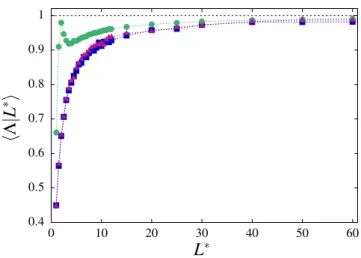
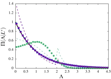
The numerical results for the normalized average chord length hΛ∗|L∗i = hΛ|L∗i/hΛi∞as a function of the normalized linear size L∗= L/hΛi∞of the do-main are illustrated in Fig.1for different mixing statistics m. Monte Carlo sim-ulation results for the chord length distribution are shown in Fig.2, for hΛi∞= 1 and for several values of L. For small L, finite-size effects are visible in the
215
chord length distribution: indeed, the longest length that can be drawn across a box of linear size L is√3L, which thus induces a cut-off on the distribution. For large L, the finite-size effects due to the cut-off fade away. In particular, the probability density for Poisson tessellations eventually converges to the expected exponential behaviour. Simulations show that the chord length distributions in
220
Box tessellations and in Poisson tessellations are very close, which is consis-tent with the observations in (Ambos and Mikhailov, 2011). On the contrary, in Voronoi tessellations, the probability density has a distinct non-exponential functional form (see Fig.2).
2.6. Assigning material compositions: colored geometries
225
In order to describe the fuel pin fragmentation that will be discussed in the next section, the material compositions of the fuel pin components must be (ran-domly) transferred to the stochastic tessellation. For the sake of simplicity, we will assume that only three compositions are present, namely the fuel, the
0.4 0.5 0.6 0.7 0.8 0.9 1 0 10 20 30 40 50 60 hΛ |L ∗ i L∗
Figure 1: Average chord length hΛ|L∗i (arbitrary units) as a function of the rescaled system size L∗= L/hΛi∞, with parameter hΛi∞= 1. Blue squares
de-note the results for Poisson tessellations, red triangles for Box tessellations, and green circles for Voronoi tessellations. Dotted lines have been added to guide the eye. Dashed black line corresponds to the asymptotic value for infinite tessella-tions.
cladding and the moderator. This procedure can be achieved by adopting ternary
230
stochastic mixtures, which are realized as follows. First, Poisson, Voronoi or Box tessellations are constructed as described above. Then, each polyhedron of the geometry is assigned a material composition by formally attributing a distinct ‘label’ (also called ‘color’), say ‘α’, ‘β ’ or ‘γ’, with associated probabilities pα,
pβ and pγ = 1 − pα− pβ. We will call a ‘cluster’ the collection of adjacent
235
polyhedra sharing the same label.
After assigning colors to stochastic geometries, we can introduce the average chord length through clusters with label i (i = α, β or γ), denoted by hΛii∞. For
infinite tessellations, it can be shown that hΛii∞ is related to the average chord
length hΛi∞of the geometry via
hΛi∞= (1 − pi)hΛii∞. (2)
This property stems from the binomial distribution of the coloring procedure ( Ha-ran et al.,2000;Larmier et al.,2016), and holds true for each tessellation m. Ad-ditionally, the corresponding probability density ΠP(Λi) is still exponential for
0 0.2 0.4 0.6 0.8 1 1.2 1.4 0 0.5 1 1.5 2 2.5 3 3.5 4 4.5 Π (Λ |L ∗ ) Λ
Figure 2: The probability density Π(Λ) of the chord length for hΛi∞= 1 as a
function of the system size L (Λ and L are given in arbitrary units). Results for Poisson tessellations are displayed in blue, Box tessellations in red, and Voronoi tessellations in green. Dashed lines correspond to L = 2. Symbols correspond to L = 100. The exponential distribution is shown as a black solid line, for reference.
infinite Poisson geometries, i.e., ΠP(Λi) =
1 hΛii∞
e−Λi/hΛii∞ (3)
For Voronoi and Box tessellations, the full probability densities ΠV(Λi) and
ΠB(Λi) are not known.
3. A model of assembly with fragmented fuel pins
The stochastic tessellations described above can be conveniently adopted to
240
represent a partially melted fuel assembly, the size of the fuel fragments being determined by the geometry density (which is a free parameter of the model). We propose in the following some benchmark configurations that are simple enough to enable a physical interpretation of the effects induced by the presence of random material fragmentation, and yet retain the key ingredients.
245
As a reference configuration we will consider an assembly composed of 17 × 17 square fuel pin-cells of side length δ = 1.262082 cm in the plane Oxy and
Material Isotopes Concentration (atoms × 1024× cm−3) UOX fuel U235 8.4148 × 10⁻⁴ U238 2.1625 × 10⁻² O16 4.4932 × 10⁻² MOX fuel U234 3.9390 × 10⁻⁷ U235 4.9524 × 10⁻⁵ U238 2.1683 × 10⁻² PU238 2.2243 × 10⁻⁵ PU239 7.0164 × 10⁻⁴ PU240 2.7138 × 10⁻⁴ PU241 1.3285 × 10⁻⁴ PU242 6.6984 × 10⁻⁵ AM241 1.2978 × 10⁻⁵ AM242M 2.2569 × 10⁻¹⁰ O16 4.5882 × 10⁻² Moderator H1 4.7716 × 10⁻² O16 2.3858 × 10⁻² B10 3.9724 × 10⁻⁶ B11 1.5890 × 10⁻⁵ Cladding ZR90 2.2060 × 10⁻² ZR91 4.8107 × 10⁻³ ZR92 7.3532 × 10⁻³ ZR94 7.4518 × 10⁻³ ZR96 1.2005 × 10⁻³
Table 2: Material compositions for the UOX and MOX assemblies used for the benchmark configurations.
of height Lz = 10 cm. Reflective boundary conditions will be imposed on all
sides of the assembly. The fuel elements will be entirely either of the UOX or MOX type: the respective material compositions for the fuel, the cladding and
250
the moderator are provided in Tab.2. The proposed compositions correspond to fresh (Beginning Of Life) fuel. The assembly will be assumed to be at a uniform temperature of T = 300 K, for conservatism (Doppler effect on reactivity will be reduced).
The partial melting of a collection of fuel pins is then introduced by applying a stochastic ternary mixing model of Poisson, Voronoi or Box type to a central region composed of nx× ny cells. For the sake of simplicity, this region will be
assumed to be located at the center of the assembly, with nx = ny= n, n being
by a stochastic tessellation. The tessellation is then randomly ‘colored’ with ternary labels, namely, ’F ’ for fuel, ’C ’ for cladding and ’M ’ for moderator, with corresponding coloring probabilities pF, pC and pM chosen so that for each material i the ensemble-averaged volumic ratio hpii coincides with that of
a pin-cell before fragmentation:
pF = πR21/δ2≈ 0.335861 pC = π(R22− R2
1)/δ2 ≈ 0.107943
pM = (δ2 − πR2
2)/δ2≈ 0.556196. (4)
Moreover, in order for the three stochastic tessellation models to yield
compara-255
ble results with respect to neutron transport, we have set the free parameters of each model (i.e., the geometry density ρ) so as to have exactly the same average chord length hΛi∞. In-pile and out-of-pile experiments of core degradation show that the fuel fragments after melting are partially mixed with the cladding (Hagen
and Hofmann,1987;Hofmann, 1999): nonetheless, for the present benchmark
260
we assume that the fuel and the cladding are present in distinct phases. The pin-cells surrounding the perturbed region are left unchanged.
It is important to note that, for a single geometrical realization, the volumic ratio of material i in the tessellation is not rigorously equal to pi, because of
finite-size effects. However, the finite-size effects progressively fade away with
265
increasing fragmentation of the tessellation, and become negligible for tessella-tions dense enough. This behaviour will be discussed in Sec.4.8.
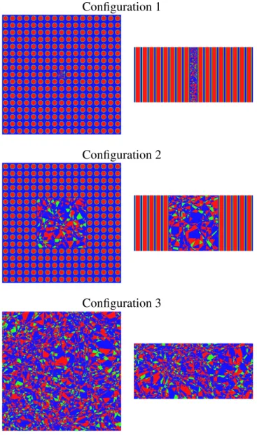
For our benchmark model, we have selected three fragmented configurations, each corresponding to a different size for the melted portion of the assembly: in configuration 1, only the central pin-cell is replaced by a ternary mixing (n = 1).
270
In configuration 2, we have chosen a portion n = 7, i.e., about half of the assem-bly is fragmented. Finally, in configuration 3, the entire assemassem-bly is fragmented (n = 17). For illustration, some of the resulting partially melted assemblies are shown in Figs.3and4.
The physical observables that we would like to determine are the
ensemble-275
averaged multiplication factor hkeffi, the ensemble-averaged kinetics parameters
(namely, the effective neutron generation time h`effi and the effective delayed
neutron fraction hβeffi), as well as and the ensemble-averaged scalar particle flux
hϕ(r, E)i within the assembly.
Our goal is to investigate how these physical observables are affected by the
280
presence of the fragmented fuel pins. For this purpose, we will vary the mixing statistics by separately testing Poisson, Voronoi and Box tessellations, and the average chord length hΛi∞for each tessellation (which basically rules the
Configuration 1
Configuration 2
Configuration 3
Figure 3: Assemblies with Poisson tessellation for the central fuel pins. Top: configuration 1 (n = 1), with hΛi∞= 0.05 cm. Center: configuration 2 (n = 7),
with hΛi∞= 0.2 cm. Bottom: configuration 3 (n = 17), with hΛi∞= 0.15 cm.
Left column: radial view. Right column: axial view.
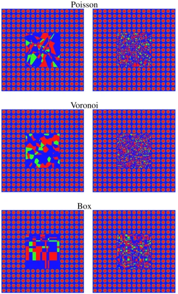
age size of the material chunks composing the randomized portion of the assem-bly). In-core experiments have shown that the fragment size may vary between
285
Poisson
Voronoi
Box
Figure 4: Assemblies with stochastic tessellation for the central fuel pins. Radial view of the configuration 2 (n = 7), for different mixing statistics and average chord lengths hΛi∞. Top: Poisson tessellation. Center: Voronoi tessellation.
Bottom: Box tessellation. Left column: hΛi∞= 0.5 cm. Right column: hΛi∞=
0.1 cm.
speed (Hagen and Hofmann,1987;Broughton et al.,1989;Hofmann,1999). De-creasing hΛi∞ means increasing the density of the tessellations, which implies
an increasing computational cost for both the generation of the random geome-try, and for the particle transport within the geometry. We have thus a practical
290
limitation to the smallest achievable value of hΛi∞. When on the contrary hΛi∞
becomes comparable to the linear size of the fragmented region, the realization of the ternary mixing are entirely dominated by finite-size effects, the disper-sion of the volumic ratio for each material composition becomes relevant. This roughly defines the upper limit for the range of hΛi∞that will be considered in
295
the numerical simulations presented in the following.
On the basis of these considerations, we have adapted the range of hΛi∞to
each configuration: for n = 1, we have taken hΛi∞from 0.03 cm to 0.5 cm; for
n= 7, we have taken hΛi∞from 0.1 cm to 1.5 cm; and for n = 17 we have taken
hΛi∞from 0.15 cm to 3 cm. Some examples of realizations of Poisson, Voronoi
300
and Box tessellations corresponding to different values of hΛi∞are displayed in
Fig.4for the benchmark configuration with n = 7.
For any mixing statistics, we will consider also the limit case of hΛi∞→ 0.
This corresponds to the so-called ‘atomic mix’ approximation, where material chunks are assumed to be so fine with respect to the average neutron free path that
305
the stochastic tessellations can be replaced by a homogenized composition where the macroscopic cross sections are obtained by averaging the cross sections of each material weighed by the respective volumic ratios: PF for the fuel, PM for the moderator, and PC for the cladding.
4. Simulation results
310
In this section we present and discuss the criticality calculations performed with TRIPOLI-4 R for the partially melted assemblies. The reference solutions
for the ensemble-averaged multiplication factor hkeffi, kinetics parameters h`effi
and hβeffi, and scalar neutron flux hϕ(r, E)i have been computed as follows. For each assembly configuration, a large number M of geometries has been gener-ated, and the material properties have been attributed to each volume as described above. Then, for each realization j of the ensemble, eigenvalue calculations have been carried out by using TRIPOLI-4 R. The number of simulated particle
his-tories per configuration has been chosen so that the statistical error on the com-puted eigenvalue keffis smaller than 50 pcm. For a given physical observableO, the benchmark solution is obtained as the ensemble average
hOi = 1 M M
∑
j=1 Oj, (5)whereOj is the Monte Carlo estimate for the observableO obtained for the
j-th realization. The scalar flux ϕj(r, E) has been recorded by using the standard
track length estimator over a pre-defined spatial grid.
The error affecting the average observable hOi results from two separate contributions, namely, the dispersion
σG2 = 1 M M
∑
j=1 Oj2− hOi2 (6)of the observables exclusively due to the stochastic nature of the geometries and of the material compositions, and
σO2 = 1 M M
∑
j=1 σO2j, (7)which is an estimate of the variance due to the stochastic nature of the Monte Carlo method for the particle transport, σO2
j being the dispersion of a single
cal-culation (Donovan and Danon,2003;Donovan et al.,2003). The statistical error on hOi is then estimated as σ [hOi] = s σG2 M + σ 2 O. (8)
Depending on the correlation lengths and on the volumetric fractions, the physical observables might display a larger or smaller dispersion around their
av-315
erage values. In order to assess the impact of such dispersion, we have also com-puted the full distribution of keff based on the available realizations. The number
of realizations M has been adapted to the configuration (i.e., to the number n of fragmented fuel pins) and to the chosen average chord length hΛi∞. As a general
remark, decreasing the average chord length hΛi∞ for a given tessellation
im-320
plies an increasing computational burden (each realization takes longer both for generation and for Monte Carlo transport), but also a better statistical averaging (a single realization is more representative of the ‘typical’ random behaviour). The parameter M varies between M = 100 for, e.g., n = 1 and hΛi∞= 0.03 cm,
and M = 3000 for, e.g., n = 17 and hΛi∞= 3 cm.
325
4.1. The TRIPOLI-4 code and the simulation options TRIPOLI-4 R
is a general-purpose Monte Carlo radiation transport code de-veloped at CEA and devoted to shielding, reactor physics with depletion, crit-icality safety and nuclear instrumentation (Brun et al., 2015). TRIPOLI-4 R is
the reference Monte Carlo code for CEA (including laboratories and reactor
fa-330
cilities) and the French utility company EDF. It is also the reference code of the CRISTAL Criticality Safety package (Gomit et al.,2011) developed with IRSN and AREVA. The code offers both fixed-source and criticality simulation modes. Neutrons are simulated in the energy range from 20 MeV to 10−5 eV. Particle transport is performed in continuous-energy, and the necessary nuclear data (i.e.,
335
point-wise cross-sections, scattering kernels, secondary energy-angle distribu-tions, secondary particle yields, fission spectra, and so on) are read by the code from any evaluation written in ENDF-6 format (McLane,2004). The code can directly access files in ENDF and PENDF format.
For the criticality calculations presented in the following, we have selected
340
the JEFF-3.1.1 nuclear data library (Santamarina et al., 2009). Concerning probability tables for the unresolved resonance range, TRIPOLI-4 R adopts the CALENDF code (Sublet et al., 2011). Thermal data S(α, β ) for bound hydro-gen in water were available in JEFF-3.1.1 at 296 K. Doppler broadening of elastic scattering differential cross sections has been enforced by using the
stan-345
dard SVT model. The DBRC model for resonant nuclides, although available in TRIPOLI-4 R
(Zoia et al., 2012), has not been used, since it is not expected to have a major impact on reactivity and kinetics parameters at low temperature.
Concerning kinetics parameters calculations, starting from version 4.10 the Iterated Fission Probability (IFP) method has been implemented in TRIPOLI
-350
4 R (Truchet et al., 2015) and extensively validated (Truchet et al., 2015; Zoia
and Brun,2016;Zoia et al., 2016). Exact calculation of adjoint-weighted quan-tities by the IFP method establishes Monte Carlo simulation as a reference tool for the analysis of effective kinetics parameters, which are key to nuclear re-actor safety during transient operation and accidental excursions (Nauchi and
355
Kameyama, 2010; Kiedrowski, 2011b). In TRIPOLI-4 R
, a superposed-cycles implementation has been chosen for IFP, with an arbitrary number of latent gen-erations M (Truchet et al.,2015). For all the simulations discussed here, we have chosen M = 20.
For our simulations, we have largely benefited from a feature that has been
360
recently implemented in the code TRIPOLI-4 R, namely the possibility of
ex-ploiting pre-computed connectivity maps for the volumes composing the geom-etry. During the generation of the stochastic tessellations, care has been taken so as to store the indexes of the neighbouring volumes for each realization, which means that during the geometrical tracking a particle will have to find the
fol-365
lowing crossed volume in a list that might be considerably smaller than the total number of random volumes composing the box (depending on the features of the
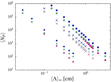
101 102 103 104 105 106 10−1 100 hN P i hΛi∞[cm]
Figure 5: Average number of polyhedra hNPi of the stochastic tessellation as a
function of the average chord length hΛi∞and of the mixing statistics m. Blue
symbols denote the results for Poisson tessellations, red symbols for Box tessel-lations, and green symbols for Voronoi tessellations. Diamonds correspond to configuration 1 (n = 1), crosses to configuration 2 (n = 7) and circles to config-uration 3 (n = 17).
random geometry).
4.2. Complexity and computer time
Before addressing the simulation results for the ensemble-averaged physical
370
observables, we briefly analyse the computational cost of the performed calcu-lations as a function of the complexity of the underlying stochastic tesselcalcu-lations. Transport calculations have been run on a cluster based at CEA, with Xeon E5-2680 V2 2.8 GHz processors. The average number of polyhedra hNPi pertaining
to each random geometry is reported in Fig.5: it is apparent that the quantity
375
hNPi increases with decreasing hΛi∞, i.e., with increasing fragmentation. The
scaling law is fairly independent of the mixing statistics m, and roughly goes as hNPi ∼ 1/hΛi3∞ for any m. The exponent of the scaling law stems from the
dimension d = 3. The number n of fragmented fuel pins does not affect these results, as expected.
380
The corresponding (ensemble-averaged) computer times for each assembly configuration are reported in Tab.3. Dispersions σ [t] are also given. The simu-lation time increases when increasing the portion of the assembly that is subject
minhΛi∞ maxhΛi∞
n tmix m hti ± σ [t] hti ± σ [t]
P 6170 ± 570 2970 ± 40 1 3260 V 4580 ± 110 2940 ± 25 B 4060 ± 225 2960 ± 30 P 18000 ± 3000 2840 ± 60 7 2990 V 9200 ± 150 2820 ± 30 B 7500 ± 1000 2840 ± 40 P 48000 ± 16000 2200 ± 200 17 1350 V 14000 ± 300 2300 ± 200 B 16000 ± 3000 2200 ± 200
Table 3: Average computer time hti (expressed in seconds) and the correspond-ing standard deviation σ [t] for transport simulations in benchmark configura-tions n = 1, n = 7 and n = 17 with UOX fuel, as a function of the mixing statistics m, for the minimal (respectively, maximal) value of the chord length minhΛi∞ (respectively, maxhΛi∞). The computer time tmix (expressed in
sec-onds) for transport simulations corresponding to atomic mix fuel fragmentation is also displayed. For reference, the computer time for a transport simulation in the UOX assembly with intact fuel pins is equal to 3240 seconds.
to fragmentation, as expected. While a decreasing trend for hti as a function of hΛi∞ is clearly apparent, subtle effects due to correlation lengths and volume
385
fractions for the material compositions come also into play, and strongly influ-ence the average computer time. For some configurations, the dispersion σ [t] may become very large, and even be comparable to the average hti. The chosen tessellation model visibly affects the computer time. Atomic mix simulations are based on a single homogenized realization, and the dispersion is thus
triv-390
ially zero.
4.3. Multiplication factor
We begin our analysis by considering the behaviour of the multiplication factor hkeffi, whose evolution is illustrated in Figs. 6, 7, and 8 for UOX and
MOX assemblies with n = 1, n = 7 and n = 17 melted fuel pins, respectively.
395
The computed value hkeffi is displayed as a function of increasing chord length
hΛi∞, for Poisson, Voronoi and Box tessellations. As detailed above, the error
bar on hkeffi results from the contribution of the Monte Carlo statistical error
1.328 1.329 1.33 1.331 1.332 1.333 1.334 0 0.1 0.2 0.3 0.4 0.5 0.6 hkef f i hΛi∞[cm] 1.155 1.156 1.157 1.158 1.159 1.16 1.161 1.162 0 0.1 0.2 0.3 0.4 0.5 0.6 hkef f i hΛi∞[cm]
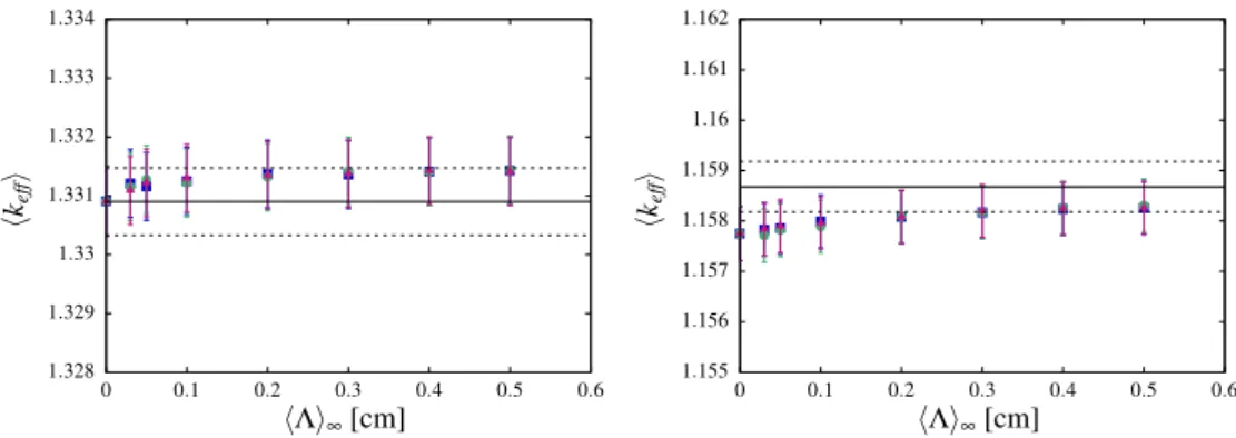
Figure 6: Evolution of the ensemble-averaged multiplication factor hkeffi as a
function of the average chord length hΛi∞. Left: UOX assembly with n = 1.
Right: MOX assembly with n = 1. Blue squares denote the results for Poisson tessellations, red triangles for Box tessellations, and green circles for Voronoi tessellations. The limit case at hΛi∞= 0 corresponds to the atomic mix model.
The black solid line denotes keff,0, the result for the assembly with intact fuel pins,
which has been added for reference (dashed lines represent the 1σ statistical uncertainty).
due to the random realizations. The limit case of atomic mix (hΛi∞→ 0) is also
400
shown. In each figure, the keff,0 eigenvalue corresponding to an assembly with
intact fuel pins is plotted for reference.
As expected on physical grounds, the impact of the stochastic tessellations on the multiplication factor depends on the size of the assembly that has been randomly fragmented. When n = 1, the difference between hkeffi and the
refer-405
ence keff,0is of the order of 100 pcm, and falls almost within 1σ uncertainty. The
major contribution to the dispersion of the multiplication factor stems from the statistical error. In this case, the impact of the specific tessellations models is not appreciable. For UOX assemblies, the average values hkeffi lie all slightly above
keff,0 for any hΛi∞, and seem to attain keff,0in the atomic mix limit. For MOX
as-410
semblies, the average values hkeffi lie all slightly below keff,0 for any hΛi∞, even
in the atomic mix limit.
When n = 7, a relevant portion of the fuel pins is fragmented, and the im-pact of the stochastic tessellations on the eigenvalue becomes apparent. For both UOX and MOX assemblies, in the atomic mix limit hkeffi is well below
415
the reference keff,0 (about 1000 pcm for UOX and 2000 pcm for MOX). Then,
for increasing chord length hΛi∞, for all the stochastic tessellations models hkeffi
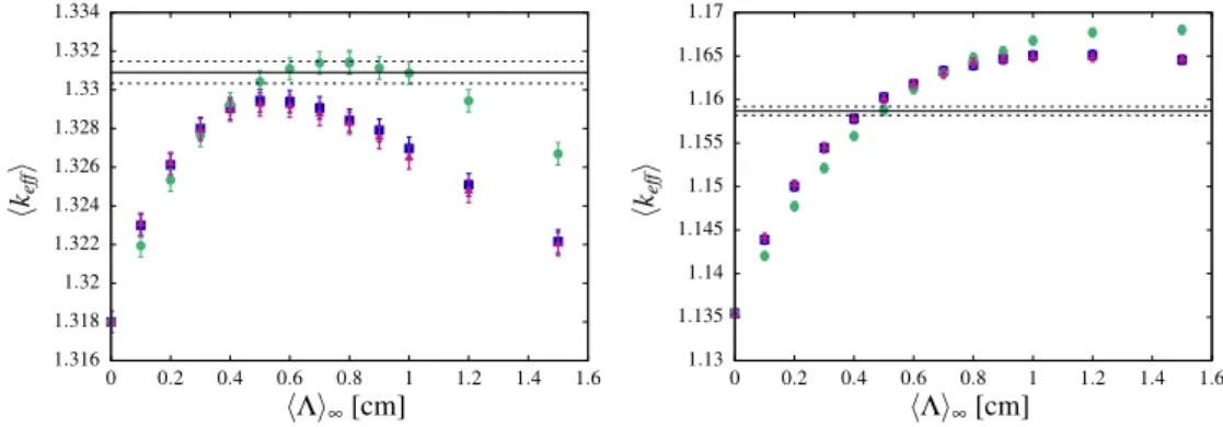
1.316 1.318 1.32 1.322 1.324 1.326 1.328 1.33 1.332 1.334 0 0.2 0.4 0.6 0.8 1 1.2 1.4 1.6 hkef f i hΛi∞[cm] 1.13 1.135 1.14 1.145 1.15 1.155 1.16 1.165 1.17 0 0.2 0.4 0.6 0.8 1 1.2 1.4 1.6 hkef f i hΛi∞[cm]
Figure 7: Evolution of the ensemble-averaged multiplication factor hkeffi as a
function of the average chord length hΛi∞. Left: UOX assembly with n = 7.
Right: MOX assembly with n = 7. Blue squares denote the results for Poisson tessellations, red triangles for Box tessellations, and green circles for Voronoi tessellations. The limit case at hΛi∞= 0 corresponds to the atomic mix model.
The black solid line denotes keff,0, the result for the assembly with intact fuel pins,
which has been added for reference (dashed lines represent the 1σ statistical uncertainty).
first increases up to a maximum value, and then decreases for even larger chord lengths. In the limit of very large hΛi∞, the stochastic tessellations would be
triv-ially filled with a single material (fuel, cladding, or moderator), each appearing
420
with its respective coloring probability. In this case, hkeffi would be the weighted
sum of the multiplication factors of three configurations with the central por-tion of the assembly replaced by a fuel, cladding or moderator zone. The values hkeffi computed for Poisson and Box tessellations are almost indistinguishable,
which supports our previous analysis. On the contrary, the hkeffi obtained for
425
the Voronoi tessellations reach their maximum for a hΛi∞larger than in the case
of the other two tessellations. The hkeffi for Voronoi tessellations lie first
be-low those of the Poisson and Box tessellations; after that hkeffi has attained its
maximum for the Poisson and Box tessellations, the values corresponding to Voronoi tessellations lie above the others. For the UOX assemblies, the
maxi-430
mum hkeffi for Poisson and Box tessellations (for hΛi∞∼ 0.5 cm) is about 300
pcm lower than keff,0, whereas for Voronoi tessellations (for hΛi∞∼ 0.7 cm) is
slightly higher. For MOX assemblies, the maxima are attained for larger average chord lengths (hΛi∞∼ 1 cm for Poisson and Box tessellations and Λ ∼ 1.6 cm
for Voronoi tessellations) and are largely higher than the reference keff,0by about
1 1.05 1.1 1.15 1.2 1.25 1.3 1.35 0 0.5 1 1.5 2 2.5 3 3.5 hkef f i hΛi∞[cm] 1 1.02 1.04 1.06 1.08 1.1 1.12 1.14 1.16 1.18 1.2 1.22 0 0.5 1 1.5 2 2.5 3 3.5 hkef f i hΛi∞[cm]
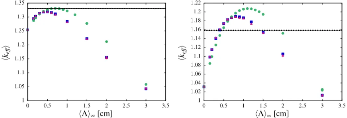
Figure 8: Evolution of the ensemble-averaged multiplication factor hkeffi as a
function of the average chord length hΛi∞. Left: UOX assembly with n = 17.
Right: MOX assembly with n = 17. Blue squares denote the results for Poisson tessellations, red triangles for Box tessellations, and green circles for Voronoi tessellations. The limit case at hΛi∞= 0 corresponds to the atomic mix model.
The black solid line denotes keff,0, the result for the assembly with intact fuel pins,
which has been added for reference (dashed lines represent the 1σ statistical uncertainty).
500 pcm.
The behaviour of the case n = 17, where the entire collection of fuel pins in the assembly is fragmented, is similar to that of the case n = 7. The position of the maxima of hkeffi as a function of the average chord length hΛi∞is almost
un-changed. The range of excursion of hkeffi in the explored domain is nonetheless
440
much larger. The eigenvalue corresponding to the atomic mix limit is lower by about 5000 pcm for the UOX case, and by about 12000 pcm for the MOX case. For UOX, the maxima of hkeffi fall below (for Poisson and Box tessellations)
or slightly above (for Voronoi tessellations) the reference keff,0. For MOX, the
maxima exceed keff,0 by about 2000 pcm for Poisson and Box tessellations, and
445
by about 4000 pcm for Voronoi tessellations.
It is interesting to remark that the behaviour of hkeffi as a function of hΛi∞
has been examined in (Pomraning, 1999) for mono-energetic transport in a rod geometry with Poisson mixing statistics: by resorting to an ingenuous perturba-tive approach, it was concluded that hkeffi ≥ keff,am for hΛi∞→ 0, where keff,am
450
is the eigenvalue corresponding to a (non-stochastic) atomic mix fragmentation. This result seems to hold also in the configurations examined here.
600 650 700 750 800 0 0.1 0.2 0.3 0.4 0.5 0.6 hβ ef f i [pcm] hΛi∞[cm] 300 350 400 450 500 0 0.1 0.2 0.3 0.4 0.5 0.6 hβ ef f i [pcm] hΛi∞[cm]
Figure 9: Evolution of the ensemble-averaged effective delayed neutron fraction hβeffi as a function of the average chord length hΛi∞. Left: UOX assembly with
n= 1. Right: MOX assembly with n = 1. Blue squares denote the results for Poisson tessellations, red triangles for Box tessellations, and green circles for Voronoi tessellations. The limit case at hΛi∞= 0 corresponds to the atomic mix
model. The black solid line denotes βeff,0, the result for the assembly with intact
fuel pins, which has been added for reference (dashed lines represent the 1σ statistical uncertainty).
4.4. Delayed neutron fraction
The evolution of the effective delayed neutron fraction hβeffi is illustrated
in Figs. 9, 10, and 11 for UOX and MOX assemblies with n = 1, n = 7 and
455
n= 17 melted fuel pins, respectively. The computed value hβeffi is displayed
as a function of increasing chord length hΛi∞, for Poisson, Voronoi and Box
tessellations. The error bar on hβeffi is of the order of about 1% of the average,
which is comparable with the uncertainty stemming from the IFP calculation for the reference assembly. The limit case of atomic mix (hΛi∞→ 0) is also shown.
460
In each figure, the βeff,0eigenvalue corresponding to an assembly with intact fuel
pins is plotted for reference.
For all the assembly configurations, the impact of stochastic tessellations on hβeffi is only marginal, and in most cases well within error bars. For UOX
assemblies we remark nonetheless that the random fragmentation introduces a
465
slight bias on the average value, i.e., hβeffi ≤ βeff,0, where βeff,0 is the reference
value corresponding to an assembly with intact fuel pins. On the contrary, for MOX assemblies hβeffi ' βeff,0.
The behaviour of hβeffi is almost unaffected by the choice of the mixing
statistics. Similarly, the average chord length hΛi∞ plays no role, and the
600 650 700 750 800 0 0.2 0.4 0.6 0.8 1 1.2 1.4 1.6 hβ ef f i [pcm] hΛi∞[cm] 300 350 400 450 500 0 0.2 0.4 0.6 0.8 1 1.2 1.4 1.6 hβ ef f i [pcm] hΛi∞[cm]
Figure 10: Evolution of the ensemble-averaged effective delayed neutron frac-tion hβeffi as a function of the average chord length hΛi∞. Left: UOX assembly
with n = 7. Right: MOX assembly with n = 7. Blue squares denote the results for Poisson tessellations, red triangles for Box tessellations, and green circles for Voronoi tessellations. The limit case at hΛi∞= 0 corresponds to the atomic
mix model. The black solid line denotes βeff,0, the result for the assembly with
intact fuel pins, which has been added for reference (dashed lines represent the 1σ statistical uncertainty).
sulting hβeffi show a slight increasing trend only for the case n = 17. Actually,
the effective delayed neutron fraction hβeffi depends mostly on the volumic
frac-tion of fuel within the assembly, and this quantity is basically flat as a funcfrac-tion of hΛi∞, as discussed in Sec.4.8.
4.5. Neutron generation time
475
The evolution of the effective neutron generation time h`effi is illustrated in
Figs.12,13, and14for UOX and MOX assemblies with n = 1, n = 7 and n = 17 melted fuel pins, respectively. The computed value h`effi is displayed as a
func-tion of increasing chord length hΛi∞, for Poisson, Voronoi and Box tessellations.
The error bar on h`effi is of the order of about 0.1% of the average, which is
com-480
parable with the uncertainty stemming from the IFP calculation for the reference assembly. The limit case of atomic mix (hΛi∞→ 0) is also shown. In each figure,
the `eff,0 eigenvalue corresponding to an assembly with intact fuel pins is plotted for reference.
As expected, in the case n = 1 the impact of the stochastic tessellations is
485
small, and the discrepancy between h`effi and `eff,0 lies within the error bar. For UOX assemblies, the random fragmentation induces h`effi ≤ `eff,0 for any hΛi∞,
600 650 700 750 800 0 0.5 1 1.5 2 2.5 3 3.5 hβ ef f i [pcm] hΛi∞[cm] 300 350 400 450 500 0 0.5 1 1.5 2 2.5 3 3.5 hβ ef f i [pcm] hΛi∞[cm]
Figure 11: Evolution of the ensemble-averaged effective delayed neutron frac-tion hβeffi as a function of the average chord length hΛi∞. Left: UOX assembly
with n = 17. Right: MOX assembly with n = 17. Blue squares denote the results for Poisson tessellations, red triangles for Box tessellations, and green circles for Voronoi tessellations. The limit case at hΛi∞= 0 corresponds to the atomic mix
model. The black solid line denotes βeff,0, the result for the UOX assembly with
intact fuel pins, which has been added for reference (dashed lines represent the 1σ statistical uncertainty).
where `eff,0 is the reference value corresponding to an assembly with intact fuel
pins. On the contrary, for MOX assemblies h`effi ≥ `eff,0for any hΛi∞.
For the assembly configurations with n = 7, the effects of the fuel
fragmen-490
tation are clearly apparent for h`effi. In the atomic mix limit for small hΛi∞,
h`effi lies below `eff,0, and it gradually increases as a function of hΛi∞. The
ensemble-averaged h`effi becomes larger than `eff,0at hΛi∞' 0.3 cm for all
mix-ing statistics. Poisson and Box tessellations yield almost identical results, and the corresponding h`effi are systematically higher than those from Voronoi
tes-495
sellations. For UOX assemblies, h`effi increases by about 10% in the range of
hΛi∞explored here, whereas for MOX assemblies the increase is of the order of
20% for the same range of hΛi∞.
For the case n = 17 the behaviour of h`effi is qualitatively similar to that of
n= 7, but the excursion range as a function of hΛi∞is wider. In particular, for
500
UOX assemblies h`effi increases by about 300% in the range of hΛi∞ explored
here, whereas for MOX assemblies the increase is of the order of 600% for the same range of hΛi∞. As in the previous case, Poisson and Box tessellations yield
15.3 15.35 15.4 15.45 15.5 15.55 15.6 15.65 15.7 0 0.1 0.2 0.3 0.4 0.5 0.6 h`ef f i [µ s] hΛi∞[cm] 7.25 7.3 7.35 7.4 7.45 7.5 7.55 0 0.1 0.2 0.3 0.4 0.5 0.6 h`ef f i [µ s] hΛi∞[cm]
Figure 12: Evolution of the ensemble-averaged effective neutron generation time h`effi as a function of the average chord length hΛi∞. Left: UOX assembly with
n= 1. Right: MOX assembly with n = 1. Blue squares denote the results for Poisson tessellations, red triangles for Box tessellations, and green circles for Voronoi tessellations. The limit case at hΛi∞= 0 corresponds to the atomic mix
model. The black solid line denotes `eff,0, the result for the UOX assembly with
intact fuel pins, which has been added for reference (dashed lines represent the 1σ statistical uncertainty).
4.6. Distribution of the multiplication factor
505
In the previous sections we have focused on the ensemble-averaged physi-cal observables hkeffi, hβeffi, and h`effi, and their evolution as a function of the
mean chord length for different mixing statistics. In order to fully apprehend the dispersion of the multiplication factors around their average values due to the variability of the random geometry realizations, which is key for criticality
510
safety applications, we have also computed the histograms Π(keff). Some repre-sentative distributions are displayed in Fig.15as a function of hΛi∞for a Poisson
tessellation and in Fig.16as a function of the mixing statistics for fixed hΛi∞.
Figure15shows that the shape of the Π(keff) distribution is sensitive to the average chord length: when hΛi∞ is small, Π(keff) is almost Gaussian, with a
515
small dispersion around the average hkeffi; as hΛi∞increases, the dispersion
in-creases, and Π(keff) becomes less symmetric (in particular, a long left tail appears for large values of hΛi∞).
Figure16shows the impact of the mixing statistics on the shape of Π(keff),
for a given average chord length hΛi∞. It is apparent that the stochastic
tes-520
sellations affect not only the average values hkeffi, but also their dispersion. In
particular, for the example considered here, The Voronoi tessellation leads to a 26
15.2 15.4 15.6 15.8 16 16.2 16.4 16.6 16.8 17 17.2 0 0.2 0.4 0.6 0.8 1 1.2 1.4 1.6 h`ef f i [µ s] hΛi∞[cm] 7 7.2 7.4 7.6 7.8 8 8.2 8.4 8.6 8.8 9 9.2 0 0.2 0.4 0.6 0.8 1 1.2 1.4 1.6 h`ef f i [µ s] hΛi∞[cm]
Figure 13: Evolution of the ensemble-averaged effective neutron generation time h`effi as a function of the average chord length hΛi∞. Left: UOX assembly with
n= 7. Right: MOX assembly with n = 7. Blue squares denote the results for Poisson tessellations, red triangles for Box tessellations, and green circles for Voronoi tessellations. The limit case at hΛi∞= 0 corresponds to the atomic mix
model. The black solid line denotes `eff,0, the result for the UOX assembly with
intact fuel pins, which has been added for reference (dashed lines represent the 1σ statistical uncertainty).
Gaussian distribution rather peaked around the average value, whereas the Pois-son and Box tessellations (whose Π(keff) are almost identical) lead to more
dis-persed and asymmetric distributions, with a long left tail.
525
4.7. Scalar neutron flux
We finalize our analysis by considering the effects of fuel fragmentation on the ensemble-averaged and normalized scalar neutron flux hϕ(r, E)i. For our Monte Carlo simulations, we have defined a 17 × 17 x − y spatial mesh super-posed to the fuel pin-cells, with a single mesh along the z axis. For symmetry
530
reasons, the flux in the reference assemblies should be spatially flat, due to re-flective boundary conditions. As for the energy dependence, we have considered a 281 group mesh, covering the entire energy range of the simulation, namely 10−5 eV to 20 MeV.
The spatial behaviour of the neutron flux hϕ(r)i is shown in Fig.17for n = 1
535
in some representative UOX and MOX assemblies, respectively, and in Fig.18
for n = 7 in some representative UOX and MOX assemblies. These curves have been obtained by integrating hϕ(r, E)i over the entire energy range. The case n= 17 leads to a spatially flat neutron flux (the fragmentation is homogeneous
10 15 20 25 30 35 40 45 50 0 0.5 1 1.5 2 2.5 3 3.5 h`ef f i [µ s] hΛi∞[cm] 5 10 15 20 25 30 35 40 0 0.5 1 1.5 2 2.5 3 3.5 h`ef f i [µ s] hΛi∞[cm]
Figure 14: Evolution of the ensemble-averaged effective neutron generation time h`effi as a function of the average chord length hΛi∞. Left: UOX assembly with
n= 17. Right: MOX assembly with n = 17. Blue squares denote the results
for Poisson tessellations, red triangles for Box tessellations, and green circles for Voronoi tessellations. The limit case at hΛi∞= 0 corresponds to the atomic mix
model. The black solid line denotes `eff,0, the result for the UOX assembly with
intact fuel pins, which has been added for reference (dashed lines represent the 1σ statistical uncertainty).
and extended to the whole assembly) and will not be shown here. For all the
540
examples discussed here we have considered Poisson stochastic tessellations. For n = 1, the effects of the stochastic tessellations on the spatial shape of the neutron flux are small, and mostly extended to a neighbourhood of the frag-mented fuel pin-cell (see Fig.17). The impact is slightly larger for MOX than for UOX assemblies. The sign of the perturbation with respect to the
remain-545
ing portion of the assembly evolves as a function of hΛi∞: for small hΛi∞ the
ensemble-averaged flux close to the fragmented fuel cell lies below the value for the rest of the assembly, whereas for larger hΛi∞the flux close to the fragmented
fuel cell lies above. The value of hΛi∞ for which the ensemble-averaged
spa-tial flux is entirely flat (i.e., the stochastic tessellation has no visible effect on
550
the flux) corresponds approximately to the average chord length through a fuel pin. In other words, if the fragmentation of the random geometry is such that neutron trajectories see a homogeneous region whose average behaviour is sta-tistically compatible with the heterogeneous regions of the intact fuel cell, then the neutron flux becomes insensitive to the fragmentation.
555
When n = 7 (Fig. 18), the behaviour of the spatial flux is qualitatively sim-ilar to the previous case. The amplitude of the perturbations introduced by the
0 10 20 30 40 50 60 70 80 90 100 110 1 1.02 1.04 1.06 1.08 1.1 1.12 1.14 1.16 1.18 1.2 1.22 Π (kef f ) keff
Figure 15: Distributions of the multiplication factor keffas a function of the
aver-age chord length hΛi∞for a MOX assembly with n = 17. The mixing statistics is
a Poisson tessellation. Blue symbols correspond to hΛi∞= 0.15, green symbols
to hΛi∞= 0.2, magenta symbols to hΛi∞= 0.3, purple symbols to hΛi∞= 0.4,
red symbols to hΛi∞= 0.5, light blue symbols to hΛi∞= 0.8 and orange
sym-bols to hΛi∞= 1. Solid black line corresponds to keff,0for a MOX assembly with
intact fuel pins; dashed black line corresponds to keff for a MOX assembly with
atomic mix.
stochastic tessellations is larger, and the effect is extended on a larger portion of the assembly. Similarly as for n = 1, the MOX assemblies are more sensitive to the perturbation. Again, the sign of the perturbation with respect to the
remain-560
ing portion of the assembly depends evolves as a function of hΛi∞: for small
hΛi∞the ensemble-averaged flux close to the fragmented portion of the
assem-bly lies below the value for the rest of the assemassem-bly, whereas for larger hΛi∞the
perturbed flux lies above. As before, there exists a value of hΛi∞for which the
ensemble-averaged spatial flux is entirely flat.
565
Concerning the behaviour of the neutron flux with respect to energy, in Fig.19
we show the spatially-integrated and normalized hϕ(E)i for UOX and MOX as-semblies. We have chosen the case n = 17 with a Poisson stochastic tessellation. The impact of stochastic tessellations on hϕ(E)i is particularly apparent when examining the discrepancies with respect to the reference flux that is obtained
570
for the assemblies with intact fuel pins (see Fig.20), for both UOX and MOX assemblies. The effects on hϕ(E)i vary as a function of hΛi∞. For small hΛi∞,
hϕ(E)i lies below the reference flux in the thermal region and above for the epi-thermal and fast regions. For larger hΛi∞, hϕ(E)i lies above the reference flux
0 25 50 75 100 125 150 175 200 225 1.25 1.26 1.27 1.28 1.29 1.3 1.31 1.32 1.33 1.34 Π (kef f ) keff
Figure 16: Distributions of the multiplication factor kefffor a UOX assembly with
n= 17 and different mixing statistics. The average chord length is hΛi∞= 0.6.
Blue symbols correspond to a Poisson stochastic tessellation, green symbols to Voronoi stochastic tessellations and red symbols to Box stochastic tessellations. Solid black line corresponds to keff,0 for a UOX assembly with intact fuel pins;
dashed black line corresponds to kefffor a UOX assembly with atomic mix.
in the thermal region and below for the epi-thermal and fast regions.
575
4.8. Finite-size effects for the assembly calculations
An investigation of finite-size effects for the stochastic tessellations used above has been carried out for hΛii, the average chord length through clusters
with material composition i. For illustration, in Fig. 21 we show the case of the assembly configurations with n = 17, where hΛii is plotted as a function of
580
hΛi∞for Poisson tessellations. As hΛi∞increases, the value of hΛii obtained by
Monte Carlo simulation progressively deviates from the theoretical behaviour hΛii∞= hΛi∞/(1 − pi).
We have also computed the average volumic fraction hpii through clusters
of composition i, as a function of the average chord length hΛi∞. The
compar-585
ison with the theoretical behaviour pi (which is strictly valid only for infinite
tessellations) is shown in Fig.22for an assembly configuration with n = 17: the deviation with respect to the ideal case increases with increasing hΛi∞, as
ex-pected. In order to emphasize the role of finite-size effects, in Fig.22we have chosen to show the geometry-induced standard deviation σG on pi, as given in
590
Eq. (6), instead of the uncertainty given by Eq.8.
−15 −10 −5 0 5 10 15−15−10−5 0 5 10 15 3.44 3.445 3.45 3.455 3.46 3.465 3.47 hϕ(x, y)i x[cm] y[cm] hϕ(x, y)i −15 −10 −5 0 5 10 15−15−10−5 0 5 10 15 3.44 3.445 3.45 3.455 3.46 3.465 3.47 hϕ(x, y)i x[cm] y[cm] hϕ(x, y)i
Figure 17: Ensemble-averaged spatial flux hϕ(x, y)i (arbitrary units) as a func-tion of the average chord length hΛi∞, with Poisson mixing statistics. Left: UOX
assembly with n = 1. Purple symbols correspond to hΛi∞= 0.03, orange
sym-bols to hΛi∞= 0.05, green symbols to hΛi∞= 0.1 and red symbols to hΛi∞= 0.5.
Right: MOX assembly with n = 1. Purple symbols correspond to hΛi∞= 0.03,
orange symbols to hΛi∞= 0.05, green symbols to hΛi∞= 0.1 and red symbols
to hΛi∞= 0.5.
5. Conclusions
Stochastic tessellations provide a convenient tool for the analysis of ran-domly fragmented materials. In this paper we have proposed a methodology for the analysis of the impact of random geometries in three-dimensional fuel
assem-595
bly, with application to criticality safety for severe accidents. Based on a random geometry generator that we have recently developed for Poisson, Voronoi and Box tessellations, we were able to create large ensembles of UOX and MOX as-sembly configurations with varying portions of fragmented fuel cells. These con-figurations can be read by the Monte Carlo transport code TRIPOLI-4 R, which
600
has been used to compute the multiplication factor, the adjoint-weighted kinetics parameters, and the scalar neutron flux. Analysis of the resulting ensemble-averaged physical quantities has allowed assessing the impact of stochastic tes-sellations on the key reactor core parameters. In particular, we have determined the evolution of hkeffi, hβeffi, and h`effi as a function of the mean chord length
605
of the random geometries, which is related to the correlation length of the frag-mented portion of the assembly. The effect of varying the mixing statistics has been also examined: while Poisson and Box tessellations yield almost identi-cal results, Voronoi tessellations yield distinct results. These findings show that the three mixing statistics, while sharing the same average chord length by
−15−10−5 0 5 10 15 −15 −10 −5 0 5 10 15 3.4 3.44 3.48 3.52 3.56 hϕ(x, y)i y[cm] x[cm] hϕ(x, y)i −15−10−5 0 5 10 15 −15 −10 −5 0 5 10 15 3.4 3.44 3.48 3.52 3.56 hϕ(x, y)i y[cm] x[cm] hϕ(x, y)i
Figure 18: Ensemble-averaged spatial flux hϕ(x, y)i (arbitrary units) as a func-tion of the average chord length hΛi∞, with Poisson mixing statistics. Left: UOX
assembly with n = 7. Purple symbols correspond to hΛi∞= 0.1, orange symbols
to hΛi∞= 0.2, green symbols to hΛi∞= 0.5 and red symbols to hΛi∞= 0.7.
Right: MOX assembly with n = 7. Purple symbols correspond to hΛi∞= 0.1,
orange symbols to hΛi∞= 0.2, green symbols to hΛi∞= 0.5 and red symbols to
hΛi∞= 0.7.
truction, might yet induce subtle effects on neutron transport due tho the precise shape of their associated chord length distributions. Generally speaking, MOX assemblies seem more sensitive than UOX assemblies to the perturbations intro-duced by the stochastic tessellations.
The preliminary results presented in this work are admittedly too simplified
615
to be amenable to general conclusions concerning the behaviour of a reactor core in the presence of partially melted fuel pins. In particular, we did not ad-dress the coupling between neutron transport and thermal-hydraulics (we have assumed the temperature to be constant at 300 K in the assembly, for conser-vatism), and we focused exclusively on the stationary behaviour. The complex
620
physical-chemistry of the reactions occurring between the fuel and the cladding at high temperature have not been addressed, either. Nonetheless, our approach is fairly broad and might be extended to more complex situations. For instance, the same procedure could be applied also to the assessment of re-criticality prob-ability of out-of-pile core degradation leading to the deposition of corium debris.
625
Monte Carlo simulation, which is capable of dealing with arbitrarily shaped ge-ometries, would be particularly useful in this context.
10−7 10−6 10−5 10−4 10−3 10−2 10−1 10−12 10−10 10−8 10−6 10−4 10−2 100 102 hϕ (E )i E[MeV] 10−8 10−7 10−6 10−5 10−4 10−3 10−2 10−1 10−12 10−10 10−8 10−6 10−4 10−2 100 102 hϕ (E )i E[MeV]
Figure 19: Ensemble-averaged spectral flux hϕ(E)i (arbitrary units) as a function of the average chord length hΛi∞, with Poisson mixing statistics. Left: UOX
assembly with n = 17. Red solid line corresponds to hΛi∞= 0.15, green solid
line to hΛi∞= 0.5, orange solid line to hΛi∞= 1 and blue solid line to hΛi∞= 3.
Right: MOX assembly with n = 17. Red solid line corresponds to hΛi∞= 0.15,
green solid line to hΛi∞ = 0.5, orange solid line to hΛi∞ = 1 and blue solid
line to hΛi∞= 3. For both UOX and MOX configurations, the dotted black line
corresponds to hϕ(E)i for assemblies with intact fuel pins; the dashed purple line corresponds to hϕ(E)i for assemblies with atomic mix.
Acknowledgements TRIPOLI-4 R
is a registered trademark of CEA. The authors wish to thank ´
Electricit´e de France (EDF) for partial financial support.
630
Adams, M.L., Larsen, E.W., Pomraning, G.C., 1989. J. Quant. Spectrosc. Radiat. Transfer 42, 253-266.
Ambos, A.Yu., Mikhailov, G.A., 2011. Russ. J. Numer. Anal. Math. Modelling 26, 263-273. Brantley, P.S., Palmer, T.S., 2009. In Proceedings of the international conference on
mathemat-ics, computational methods & reactor physics (M&C2009), Saratoga Springs, New York.
635
Brantley, P.S., 2009. In Proceedings of the international conference on mathematics, computa-tional methods & reactor physics (M&C2009), Saratoga Springs, New York.
Brantley, P.S., 2011. J. Quant. Spectrosc. Radiat. Transfer 112, 599-618.
Broughton, J.M., Kuan, P., Petti, D.A., Tolman, E.L., 1989. Nucl. Techn. 87, 34-53. Brown, F.B., Martin, W.R., 2004. Ann. Nucl. Energy 31, 2039-2047.
640
Brun, E., et al., 2015. Ann. Nucl. Energy 82, 151-160.
Chiu, S.N., Stoyan, D., Kendall, W.S., Mecke, J., 2013. Stochastic geometry and its applications, Wiley, New York, USA.
Coleman, R., 1969. J. Appl. Probab. 6, 430-441.
Donovan, T.J., Danon, Y., 2003. Nucl. Sci. Eng. 143, 226-239.
![Table 3: Average computer time hti (expressed in seconds) and the correspond- correspond-ing standard deviation σ [t] for transport simulations in benchmark configura-tions n = 1, n = 7 and n = 17 with UOX fuel, as a function of the mixing statistics m, f](https://thumb-eu.123doks.com/thumbv2/123doknet/13160955.389873/20.892.292.601.211.447/expressed-correspond-correspond-deviation-transport-simulations-benchmark-statistics.webp)