Learning brain alterations in multiple sclerosis from multimodal neuroimaging data

(1)

HAL Id: tel-02862395

https://tel.archives-ouvertes.fr/tel-02862395v2

Submitted on 8 Feb 2021

Learning brain alterations in multiple sclerosis from

multimodal neuroimaging data

Wen Wei

To cite this version:

Wen Wei. Learning brain alterations in multiple sclerosis from multimodal neuroimaging data. Bio-engineering. Université Côte d’Azur, 2020. English. �NNT : 2020COAZ4021�. �tel-02862395v2�

(2)

Apprentissage Automatique des Altérations

Cérébrales Causées par la Sclérose en

Plaques en Neuro-Imagerie Multimodale

Wen Wei

INRIA, Équipes Epione et ARAMIS

Dirigée par : Nicholas Ayache, Olivier Colliot

Soutenue le : 5 Juin 2020

Présentée en vue de l’obtention du grade de docteur en AUTOMATIQUE,

TRAITEMENT DU SIGNAL ET DES IMAGES

d’UNIVERSITE COTE D’AZUR

Devant le jury, composé de :

Isabelle Bloch Pierrick Coupé Hervé Delingette Bruno Stankoff Nicholas Ayache Olivier Colliot Stanley Durrleman

Télécom Paris, France

Université de Bordeaux, France INRIA Sophia Antipolis, France ICM - Hôpital Pitié Salpêtrière, France INRIA Sophia Antipolis, France Sorbonne Université & INRIA, France INRIA & ICM, France

Rapporteur, Examinateur Rapporteur, Examinateur

Président, Examinateur Examinateur

Directeur de thèse, Examinateur Co-directeur de thèse, Invité

Invité

(3)

(4)

Apprentissage Automatique des Altérations

Cérébrales Causées par la Sclérose en

Plaques en Neuro-Imagerie Multimodale

Learning Brain Alterations in

Multiple Sclerosis from

Multimodal Neuroimaging Data

Jury :

Président du jury :

Hervé Delingette

- INRIA Sophia Antipolis, France

Rapporteurs :

Isabelle Bloch

- Télécom Paris, France

Pierrick Coupé

- Université de Bordeaux, France

Examinateurs :

Isabelle Bloch

- Télécom Paris, France

Pierrick Coupé

- Université de Bordeaux, France

Hervé Delingette

- INRIA Sophia Antipolis, France

Bruno Stankoff

- ICM - Hôpital Pitié Salpêtrière, France

Nicholas Ayache

- INRIA Sophia Antipolis, France

Invités :

Olivier Colliot

- Sorbonne Université & INRIA, France

Stanley Durrleman

- INRIA & ICM, France

(5)

(6)

Abstract

Multiple Sclerosis (MS) is the most common progressive neurological disease of young adults worldwide and thus represents a major public health issue with about 90,000 patients in France and more than 500,000 people affected with MS in Europe. In order to optimize treatments, it is essential to be able to measure and track brain alterations in MS patients. In fact, MS is a multi-faceted diseases which involves different types of alterations, such as myelin damage and repair. Under this observation, multimodal neuroimaging are needed to fully characterize the disease. Magnetic resonance imaging (MRI) has emerged as a fundamental imaging biomarker for multiple sclerosis because of its high sensitivity to reveal macroscopic tissue abnormalities in patients with MS. Conventional MR scanning provides a direct way to detect MS lesions and their changes, and plays a dominant role in the diagnostic criteria of MS. Moreover, positron emission tomography (PET) imaging, an alternative imaging modality, can provide functional information and detect target tissue changes at the cellular and molecular level by using various radiotracers. For example, by using the radiotracer [11_{C]PIB, PET allows} a direct pathological measure of myelin alteration. However, in clinical settings, not all the modalities are available because of various reasons. In this thesis, we therefore focus on learning and predicting missing-modality-derived brain alterations in MS from multimodal neuroimaging data.

Keywords: Multiple Sclerosis, PET Imaging, MR Imaging, Brain Alterations, Deep Learning, Convolutional Neural Networks (CNN), Generative Adver-sarial Network (GAN), Image Synthesis, Missing MRI Sequences, Missing Modalities

(7)

Résumé

La sclérose en plaques (SEP) est la maladie neurologique évolutive la plus courante chez les jeunes adultes dans le monde et représente donc un problème de santé publique majeur avec environ 90 000 patients en France et plus de 500 000 personnes atteintes de SEP en Europe. Afin d’optimiser les traitements, il est essentiel de pouvoir mesurer et suivre les altérations cérébrales chez les patients atteints de SEP. En fait, la SEP est une maladie aux multiples facettes qui implique différents types d’altérations, telles que les dommages et la réparation de la myéline. Selon cette observation, la neuroimagerie multimodale est nécessaire pour caractériser pleinement la maladie. L’imagerie par résonance magnétique (IRM) est devenue un biomarqueur d’imagerie fondamental pour la sclérose en plaques en raison de sa haute sensibilité à révéler des anomalies tissulaires macroscopiques chez les patients atteints de SEP. L’IRM conventionnelle fournit un moyen direct de détecter les lésions de SEP et leurs changements, et joue un rôle dominant dans les critères diagnostiques de la SEP. De plus, l’imagerie par tomographie par émission de positons (TEP), une autre modalité d’imagerie, peut fournir des informations fonctionnelles et détecter les changements tissulaires cibles au niveau cellulaire et moléculaire en utilisant divers radiotraceurs. Par exemple, en utilisant le radiotraceur [11_{C]PIB, la TEP permet une mesure} pathologique directe de l’altération de la myéline. Cependant, en milieu clinique, toutes les modalités ne sont pas disponibles pour diverses raisons. Dans cette thèse, nous nous concentrons donc sur l’apprentissage et la prédiction des altérations cérébrales dérivées des modalités manquantes dans la SEP à partir de données de neuroimagerie multimodale.

Mots clés: Sclérose en Plaques, TEP, IRM, Altérations Cérébrales, Appren-tissage en Profondeur, Réseau de Neurones Convolutifs (CNN), Réseaux Antagonistes Génératifs (GAN), Synthèse d’images, Séquences IRM Man-quantes, Modalités Manquantes

(8)

Acknowledgements

The period of my PhD has been a truly priceless life-changing experience for me and it would not have been possible to do without the support and guidance that I received from many people.

First and foremost I would like to express my sincere gratitude to my super-visors, Nicholas and Olivier, for their continuous support of my PhD study in two teams, for their patience, motivation, and immense knowledge. I appreciate all their contributions of time, ideas, and funding to make my PhD experience productive and stimulating. Many thanks to Nicholas, who not only encouraged my research, but also expertly guided and taught me to grow as a research scientist. Many thanks also to Olivier, whose advices on both research as well as on my career have been priceless. I could not have imagined having better advisors and mentors for my PhD study.

Apart from my supervisors, I won’t forget to express the gratitude to my clinical collaborators: Emilie Poirion, Bruno Stankoff, Benedetta Bodini and Matteo Tonietto, for giving the encouragement and sharing insightful suggestions. I would like also to thank Bruno for being one of the members of the thesis committee. I am especially grateful to Emilie Poirion who helped me a lot on brain image processing and answered lots of my questions about multiple sclerosis.

Then, I want to thank the reviewers of my thesis, Isabelle Bloch, and Pierrick Coupé, for reading and reviewing my manuscript, as well as for attending my thesis defense especially during this difficult time because of COVID-19.

My sincere thanks goes to all the members in the team Epione(Asclepios), including those who have already left. Thanks to Hervé, Xavier, Maxime, and Marco for answering my questions and sharing their ideas. Special thanks to Hervé for being the jury president. Many thanks to Thomas, Marc-Michel, Sophie, Pawel, Raphaël, Roch, Rocio, Sofia, Julian, Shuman, Zihao, Qiao, Nina, Manon, Yann T., Nicholas G., Nicholas C., Clement, Jaume, Luigi, Sara, Buntheng, Benoit, Florent, Santiago, Yingyu, Fanny, Alan, Loic and many

(9)

others for the great time we have shared. Special thanks to Isabelle, for supporting and helping me a lot with my travels between Paris and Nice, houses, holidays, VISA and so on. I would like also to thank the members in the team ARAMIS including Ninon, Stanley, Junhao, Fabrizio, Marie-Constance, Igor, Raphael, Tiziana, Simona, Johann, Giulia, Elina, Alexandre R, Alexandre B, Manon, Pascal, Alexis, Jorge, and many others. Moreover, I acknowledge the financial support from INRIA, 3IA Côte d’Azur and ICM.

Lastly, thanks to Danny and Alexandra who treat us like their own children and we have shared unforgettable memories in Villa Plantagenet in Antibes. Many thanks to my parents in law who always encouraged me. I would like to say a heartfelt thank you to my family for all their love and encouragement. A special thanks to my lovely parents who raised me and supported me in all my pursuits. Finally I would like to express appreciation to my lovely, patient, encouraging wife Pengchi, who has been extremely supportive and always been my side throughout my PhD. Without her, my life wouldn’t complete so. And also to my darling Yanxi for choosing us as her parents and making my PhD more memorable.

Wen Wei Antibes During the COVID-19 lockdown

(10)

1

Introduction

Contents

1.1 Context . . . 1

1.1.1 Multiple Sclerosis . . . 1

1.1.2 Multimodal Neuroimaging in Multiple Sclerosis 2

1.2 Deep Learning for Medical Image Prediction . . . 3

1.2.1 Convolutional Neural Networks (CNNs) . . . . 3

1.2.2 Generative Adversarial Networks (GANs). . . . 4

1.3 Thesis overview . . . 5

1.1 Context

1.1.1 Multiple Sclerosis

Multiple Sclerosis is the most common progressive neurological disease of young adults worldwide and thus represents a major public health issue with about 90,000 patients in France and more than 500,000 people affected with MS in Europe1. This disease is an autoimmune disease in which the immune system attacks myelinated axons in the central nervous system (CNS), damaging or destroying the myelin (demyelination). This damage disrupts the ability of CNS to transmit signals, leading to various symptoms, including paralysis, sensory disturbances, lack of coordination and visual impairment [Compston, 2008]. Clinically, MS can present as different dynamic phenotypes [Lublin, 2014]:

1) Relapsing-remitting MS (RRMS), the most common disease course, is characterized by clearly defined attacks (also called relapses) followed by periods of partial or complete recovery (remissions). During remis-sions, all symptoms may disappear, or some symptoms may continue and become permanent;

1_{MS Barameter 2015: http://www.emsp.org/projects/ms-barometer/}

(15)

2) Secondary progressive MS (SPMS), develops from RRMS for many people. Patients with SPMS generally have fewer relapses and a progressive worsening of neurological function, because nerves have begun to be damaged or lost at this stage;

3) Primary progressive MS (PPMS), is characterized by worsening neuro-logical function and gradual accumulation of disability from the onset of symptoms, without early relapses or remissions.

The cause of MS is still unknown. Scientists believe that a combination of environmental and genetic factors contribute to the risk of developing MS.

1.1.2 Multimodal Neuroimaging in Multiple Sclerosis

Neuroimaging is increasingly used to help clinicians in understanding MS physiopathological mechanisms, such as myelin damage and repair, mon-itoring disease progression, and improving the accuracy of MS diagnosis and prognosis. In the last decade, magnetic resonance imaging (MRI) has emerged as a fundamental imaging biomarker for multiple sclerosis because of its high sensitivity to reveal macroscopic tissue abnormalities in patients with MS. Conventional MR scanning provides a direct way to detect MS lesions and their changes, and plays a dominant role in the diagnostic cri-teria of MS [Thompson, 2018]. In particular, T2-weighted image is highly sensitive in detection of hyperintense lesions in the white matter (WM) so that the quantification of T2 lesion load is often used to assess the dis-ease burden. As periventricular lesions are often indistinguishable from the adjacent cerebrospinal fluid (CSF) which is also of high signal on the T2-w, fluid-attenuated inversion recovery (FLAIR) is especially helpful in the evaluation of these lesions due to its ability to suppress the ventricular signal. In addition, double inversion recovery (DIR) has direct application in MS for evaluating cortical pathology. Unlike conventional MR imaging, magnetization transfer ratio (MTR) offers greater pathologic specificity for macromolecules and is utilized to measure myelin content and tissue dam-age. However, the pathological specificity of MTR is limited since the signal can be influenced by water content and inflammation.

(16)

for multiple different aspects of MS to enhance understanding the patho-physiology of the disease [Poutiainen, 2016]. For example, the radiotracer [11C]PIB is used as a myelin tracer in MS clinical settings because of its ability to selectively bind to myelinated white matter regions [Stankoff, 2011]. As mentioned above, all of these multimodal neuroimages play different roles in MS diagnosis and clinical research. However, in clinical settings, not all the modalities are available because of various reasons, such as patients’ inter-ruptions resulting in the missing of some MRI pulse sequences. In this work, we therefore focus on learning and predicting missing-modality-derived brain alterations in MS from multimodal neuroimaging data.

1.2 Deep Learning for Medical Image

Prediction

In the recent years, deep learning has achieved state-of-the-art results in vari-ous areas including computer vision and medical image analysis. In addition, benefit from modern hardware and software resource, deep learning models can be trained very fast and applied for huge high-dimensional datasets. In the particular case of medical image prediction, many researchers are trying to explore how to use deep learning methods to deal with various challenges in this field. Among them, convolutional neural networks (CNNs) and generative adversarial networks (GANs) are two mainly used models.

1.2.1 Convolutional Neural Networks (CNNs)

The architecture of a CNN is analogous to that of the connectivity pattern of neurons in the human brain and was inspired by the organization of the visual cortex. Standard convolutional neural networks include an input, an output layer, as well as multiple hidden layers which are typically a series of convolutional layers followed by additional layers such as pooling layers, fully connected layers and normalization layers. Various methods based on CNNs have been proposed for medical image prediction, for instance, reconstruction of 7T-like images from 3T MRI [Bahrami, 2016b], synthesis of CT images from MRI [Nie, 2016], prediction of positron emission tomog-raphy (PET) images with MRI [Li, 2014], and generation of FLAIR from T1-w MRI [Sevetlidis, 2016].

Among the CNN architectures, the most commonly used framework is U-Net [Ronneberger, 2015] which has achieved competitive performance in

(17)

both computer vision [Ma, 2018;Zhang, 2018b] and medical imaging fields [Rohé, 2017; Zheng, 2018]. Benefiting from the introduced skip connec-tions in U-Net, the network is able to retrieve the spatial information lost during the down-sampling operations. In addition, the gradient vanishing problem which is a typical issue during the training process is mitigated, since the gradients from the deeper layers can be directly back-propagated to the shallower layers through the skip connections. Improved results have been shown for image prediction by using U-Net model [Han, 2017;Sikka, 2018].

1.2.2 Generative Adversarial Networks (GANs)

The original GAN was proposed by Goodfellow et al. [Goodfellow, 2014] for nature image synthesis. Different from the CNN-based models, the GAN consists of two components: a generator G and a discriminator D. The generator G is trained to generate samples which are as realistic as possible, while the discriminator D is trained to maximize the probability of assigning the correct label both to training examples from the real dataset and samples from G. This adversarial training strategy can make the synthesized image to be indistinguishable from the real ones. In order to constrain the outputs of the generator G, conditional GAN (cGAN) [Mirza, 2014] was proposed in which the generator and the discriminator both receive a conditional variable.

More recently, a lot of works using GAN-based methods have further im-proved the medical image prediction results, such as PET-to-MRI prediction for the quantification of cortical amyloid load [Choi, 2018] and CT-to-PET synthesis [Bi, 2017]. Several studies also achieved state-of-the-art results via GANs on other modality synthesis, for instance retinal images [Costa, 2018;

Zhao, 2018], ultrasound images [Hu, 2017] and endoscopy images [ Mah-mood, 2018]. Unlike optimizing a single loss function used in standard convolutional neural networks, both the generator and the discriminator in GANs have cost functions that are defined in terms of both players’ parame-ters. Because each player’s cost depends on the other player’s parameters, but each player cannot control the other player’s parameters, this scenario is

(18)

1.3 Thesis overview

In this thesis, we aim to propose efficient methods to learn and predict brain alterations in MS from multimodal neuroimaging data. The following chap-ters correspond to published or submitted articles during the preparation of the thesis.

Inchapter 2, we propose 3D fully convolutional neural networks to predict FLAIR pulse sequence from some other MRI pulse sequences, such as T1-w, T2-w, and so on. Our approach is tested on a real multiple sclerosis image dataset and evaluated by comparing our approach to other methods. As the FLAIR pulse sequence is used clinically and in research for the detection of WM lesions, we also assess the lesion contrast in the ground truth and the synthesized FLAIR pulse sequences from our method and other methods. This chapter is based on the publication [Wei, 2019a].

Inchapter 3, we aim to learn and predict myelin content which is quantified by PET imaging and is essential to understand the MS physiopathology, track progression and assess treatment efficacy. For this purpose, we propose Sketcher-Refiner GANs with specifically designed adversarial loss functions to predict the PET-derived myelin content map from multisequence MRI. A visual attention saliency map is also proposed to interpret the attention of neural networks. We compared our method with state-of-the-art methods. Particularly, it is evaluated at both global and voxel-wise levels for myelin content prediction. The work presented in this chapter is published in [Wei, 2019b]. A preliminary version of this work was presented orally at MICCAI 2018 and published in the proceedings of the conference [Wei, 2018b].

Inchapter 4, our goal is to further learn and predict myelin changes (i.e. demyelination-remyelination cycles) for MS individual longitudinal analysis. The method is based on conditional flexible self-attention GAN (cFSAGAN) which is specifically adjusted for high-dimensional medical images and able to capture the relationships between the spatially separated lesional regions during the image synthesis process. Jointly applying the sketch-refinement process described in chapter 3, the result is further improved and the method is shown to outperform the state-of-the-art methods qualitatively and quantitatively. Importantly, the clinical evaluations of our method for the prediction of myelin content for MS individual longitudinal analysis show similar results to the PET-derived gold standard. This study has been submitted to the conference MICCAI 2020 [Wei, 2020a] and the journal NeuroImage [Wei, 2020b].

(19)

Inchapter 5, we finally summarize the main contributions of the thesis and discuss the perspectives for future research work.

(20)

2

FLAIR MR Image synthesis

from Multisequence MRI

using 3D Fully Convolutional

Networks for Multiple

Sclerosis

Contents

2.1 Introduction . . . 8

2.2 Method . . . 10

2.2.1 3D Fully Convolutional Neural Networks . . . . 11

2.2.2 Pulse-sequence-specific Saliency Map (P3S Map) 12

2.2.3 Materials and Implementation Details . . . 13

2.3 Experiments and Results . . . 14

2.3.1 Model Parameters and Performance Trade-offs . 14

2.3.2 Evaluation of Predicted Images . . . 15

2.3.3 Pulse-Sequence-Specific Saliency Map (P3S Map) 16

2.4 Discussion and Conclusion . . . 20

This chapter corresponds to the following scientific articles:

• [Wei, 2019a] Fluid-attenuated Inversion Recovery MRI Synthesis from

Multisequence MRI using Three-dimensional Fully Convolutional Net-works for Multiple Sclerosis

W.Wei, E.Poirion, B.Bodini, S.Durrleman, O.Colliot, B.Stankoff, N.Ayache

Journal of Medical Imaging (JMI), 6(01):27, February 2019

• [Wei, 2018a] FLAIR MR Image Synthesis by Using 3D Fully

Convolu-tional Networks for Multiple Sclerosis

W.Wei, E.Poirion, B.Bodini, S.Durrleman, O.Colliot, B.Stankoff, N.Ayache ISMRM-ESMRMB 2018 - Joint Annual Meeting, Paris, France

(21)

2.1 Introduction

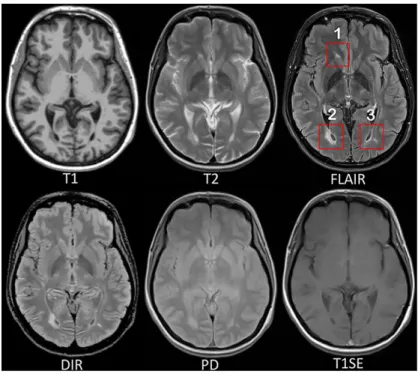
Multiple sclerosis (MS) is a demyelinating and inflammatory disease of the central nervous system and a major cause of disability in young adults [Compston, 2008]. MS has been characterized as a white matter (WM) dis-ease with the formation of WM lesions, which can be visualized by magnetic resonance imaging (MRI) [Paty, 1988;Barkhof, 1997]. The fluid-attenuated inversion recovery (FLAIR) MRI pulse sequence is commonly used clinically and in research for the detection of WM lesions which appear hyperintense compared to the normal appearing WM tissue (NAWM). Moreover, the sup-pression of the ventricular signal, characteristic of the FLAIR images, allows an improved visualization of the periventricular MS lesions [Woo, 2006], and can also suppress any artifacts created by CSF. In addition, the decrease of the dynamic range of the image can make the subtle changes easier to see. Typical MRI pulse sequences used in a clinical setting are shown in Fig.2.1. WM lesions (red rectangles) characteristic of MS are clearly best seen on FLAIR pulse sequences. However, in a clinical setting, some MRI pulse sequences can be missing because of limited scanning time or patients’ interruptions in case of anxiety, confusion or severe pain. Hence, there is a need for predicting the missing FLAIR when it has not been acquired during patients’ visits. FLAIR may also be absent in some legacy research datasets, that are still of major interest due to their number of subjects and long follow-up periods, such as ADNI [Mueller, 2005]. Furthermore, the automatically synthesized MR images may also improve brain tissue classification and segmentation results as suggested in the works of Iglesias et al. [Iglesias, 2013] and Van Tulder and Bruijne [Van Tulder, 2015], which is an additional motivation for this work.

In the work of Roy et al. [Roy, 2010], the authors proposed an atlas-based patch matching method to predict FLAIR from T1-w and T2-w. In this approach, given a set of atlas images (IT1, IT2, IFLAIR)and a subject S with (S_T1, ST2), the corresponding FLAIR ˆSFLAIRis formed patch by patch. A pair of patches in (ST1, ST2)is extracted and used to find the most similar one in the set of patches extracted from the atlas (IT1, IT2). Then the corresponding patch in IFLAIRis picked and used to form ˆSFLAIR.

In the work of Jog et al. [Jog, 2014], random forests (RF) are used to predict FLAIR given T1-w, T2-w, and PD. In this approach, a patch at position i is extracted from each of these three input pulse sequences. All these three patches are then rearranged and concatenated to form a column vector Xi.

(22)

Fig. 2.1: MRI pulse sequences usually used in a clinical setting.

T1-w provides an anatomical reference and T2-w is used for WM lesions visualization. However, on the T2-w, periventricular lesions are often indistinguishable from the adjacent cerebrospinal fluid (CSF) which is also of high signal. WM lesions (red rectangles) characteristic of MS are best seen on FLAIR pulse sequence because of the suppression of the ventricular signal. Double inversion recovery (DIR) has direct application in MS for evaluating cortical pathology. Proton density (PD) and T1 spin-echo (T1SE) are also used clinically.

used to train the RF. There are also some other close research fields doing subject-specific image synthesis of a target modality from another modality. For example, in the works of Huynh et al. [Huynh, 2016] and Burgos et al. [Burgos, 2014], computed tomography (CT) imaging is predicted from MRI pulse sequences.

Recently, deep learning has achieved state-of-the-art results in several com-puter vision domains, such as image classification [He, 2016], object detec-tion [Chen, 2017], segmentation [Shelhamer, 2017] and also in the fields of medical image analysis [Zhou, 2017]. Various methods of image enhance-ment and reconstruction using a deep architecture have been proposed, for instance, reconstruction of 7T-like images from 3T MRI [Bahrami, 2016b] and of CT images from MRI [Nie, 2016], and prediction of positron emission tomography (PET) images with MRI [Li, 2014]. The research work most similar to ours is Sevetlidis et al. [Sevetlidis, 2016]. In this method, FLAIR is generated from T1-w MRI by a five-layer 2D deep neural network (DNN) which treats the input image slice-by-slice.

(23)

However, these FLAIR synthesis methods have their own shortcomings. The method in the work of Roy et al. [Roy, 2010] breaks the input images into patches. During inference process, the extracted patch is then used to find the most similar patch in the atlas. But this process is often computationally expensive. Moreover, the result heavily depends on the similarity between the source image and the images in the atlas. This makes the method fail in the presence of abnormal tissue anatomy since the images in the atlas do not have the same pathology. The learning based methods in Refs. Jog et al. [Jog, 2014] and Sevetlidis et al. [Sevetlidis, 2016] are less computationally intensive, because they store only the mapping function. However, they do not take into account the spatial nature of 3D images and can cause discontinuous predictions between adjacent slices. Moreover, many works used multiple MRI pulse sequences as the inputs [Roy, 2010;Jog, 2014], but none of them evaluated how each pulse sequence influences the prediction results.

In order to overcome the disadvantages mentioned above, we propose 3D Fully Convolutional Neural Networks (3D FCNs) to predict FLAIR. The proposed method can learn an end-to-end and voxel-to-voxel mapping between other MRI pulse sequences and the corresponding FLAIR. Our networks have three convolutional layers and the performance is evaluated qualitatively and quantitatively. Moreover, we propose a pulse-sequence-specific saliency map (P3S map) to visually measure the impact of each input pulse sequence on the prediction result.

2.2 Method

Standard convolutional neural networks are defined for instance in Refs. Le-Cun et al. [LeCun, 1989] and Krizhevsky et al. [Krizhevsky, 2012]. Their architectures basically contain three components: convolutional layers, pool-ing layers, and fully-connected layers. A convolutional layer is used for feature learning. A feature at some locations in the image can be calcu-lated by convolving the learned feature detector and the patches at those locations. A pooling layer is used to progressively reduce the spatial size of feature maps in order to reduce the computational cost and the number of parameters. However, the use of a pooling layer can cause the loss of spatial information, which is important for image prediction, especially the lesion regions. Moreover, a fully-connected layer has all the hidden units connected to all the previous units, so it contains majority of the total parameters and an additional fully-connected layer makes it easy to reach the hardware

(24)

limits both in memory and computation power. Therefore, we propose fully convolutional neural networks composed of only three convolutional layers.

2.2.1 3D Fully Convolutional Neural Networks

Our goal is to predict FLAIR pulse sequences by finding a non-linear function

s, which maps multi-pulse-sequence source images Isource=( IT1, IT2, IPD,

IT1SE, IDIR), to the corresponding target pulse sequence Itarget. Given a

set of source images Isource, and the corresponding target pulse sequence

Itarget, our method finds the non-linear function by solving the following

optimization problem:

ˆ

s = arg min

s∈S

PN

i=1k(Itargeti , s(Isourcei ))k2

N (2.1)

where S denotes a group of potential mapping functions, N is the number of subjects and mean-square-error (MSE) is used as our loss function which calculates a discrepancy between the predicted images and the ground truth.

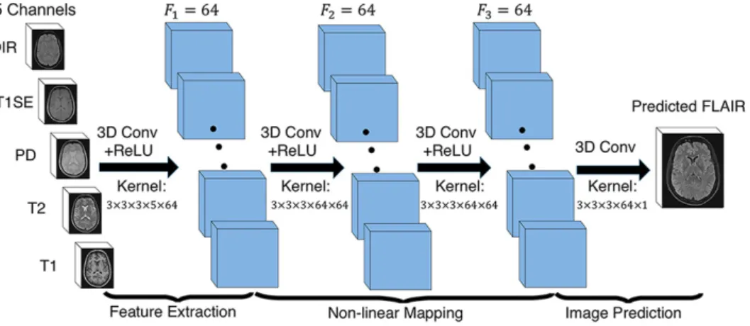
In order to learn the non-linear function, we propose the architecture of our 3D fully convolutional neural networks shown in Fig.2.2. The input layer is composed of the multi-pulse-sequence source images Isourcewhich

are arranged as channels and then sent altogether to the network. Our network architecture consists of three convolutional layers (L = 3) followed by rectified linear functions (relu(x) = max(x, 0)). If we denote the mth feature map at a given layer as hm_{, whose filters are determined by the}

weights km_{and bias b}m_{, then the feature map h}m_{is obtained as follows:}

hm = max(km∗ x + bm, 0) (2.2)

where the size of input x is H × W × D × M . Here, H, W, D indicate the height, width and depth of each pulse sequence or feature map and M is the number of the pulse sequences or feature maps. To form a richer representation of the data, each layer is composed of multiple feature maps {hm_{: 1, ..., F }, also referred as channels. Note that the kernel k has a}

dimension Hk× Wk× Dk× M × F where Hk, Wk, Dkare the height, width

and depth of the kernel respectively. The kernel k operates on x with M channels, generating h with F channels. The parameters k, b in our model

(25)

can be efficiently learned by minimizing the function2.1using stochastic gradient descent (SGD).

Fig. 2.2: The proposed 3D fully convolutional neural networks.

Our network architecture consists of three convolutional layers. The input layer is composed of 5 pulse sequences arranged as channels. The first layer extracts a 64-dimensional feature from input images through convolution process with a 3 × 3 × 3 × 5 × 64 kernel. The second and third layers apply the same convolution process to find a non-linear mapping for image prediction.

2.2.2 Pulse-sequence-specific Saliency Map (P3S

Map)

Multiple MRI pulse sequences are used as inputs to predict FLAIR. Given a set of input pulse sequences and a target pulse sequence, we would like to assess the contribution of each pulse sequence on the prediction result. One method is class saliency visualization proposed in the work of Simonyan et al. [Simonyan, 2013], which is used for image classification to see which pixels influence the most the class score. Such pixels can be used to locate the object in the image. We call the method presented in this paper pulse-sequence-specific saliency map to visually measure the impact of each pulse sequence on the prediction result. Our P3S map is the absolute partial derivative of the difference between the predicted image and the ground truth with respect to the input pulse sequence of subject i. It is calculated by standard backpropagation. Mi=

∂kI_targeti − ˆI_targeti k₂

∂Ii source (2.3)

where i denotes the subject, Itargetand ˆItargetare the ground truth and the

(26)

2.2.3 Materials and Implementation Details

Our dataset contains 24 subjects including 20 MS patients (8 women, mean age 35.1, sd 7.7) and 4 age- and gender-matched healthy volunteers (2 women, mean age 33, sd 5.6). Each subject underwent the following pulse sequences:

a) T1-w (1 × 1 × 1.1mm3₎

b) T2-w and Proton Density (PD) (0.9 × 0.9 × 3mm3₎ c) FLAIR (0.9 × 0.9 × 3mm3₎

d) T1 spin-echo (T1SE, 1 × 1 × 3mm3₎

e) Double Inversion Recovery (DIR, 1 × 1 × 1mm3₎

All have signed written informed consent to participate in a clinical imag-ing protocol approved by the local ethics committee. The preprocess-ing steps include intensity inhomogeneity correction [Tustison, 2010] and intra-subject affine registration [Greve, 2009] onto FLAIR space. Finally, each preprocessed image has a size of 208 × 256 × 40 and a resolution of 0.9 × 0.9 × 3mm3_.

Our networks have three convolutional layers (L = 3). The filter size is 3 × 3 × 3 and for every layer the number of the filters is 64 which is designed with empirical knowledge from the widely-used FCN architectures, such as ResNet [He, 2016]. We used Theano [Theano, 2016] and Keras [Chollet, 2015] libraries for both training and testing. The whole data is first normalized by using ¯x = (x − mean)/std, where mean and std are calculated over all the voxels of all the images in each sequence. We do not use any data augmentation. Our networks were then trained using standard SGD optimizer with 0.0005 as the learning rate and 1 as the batch size. The stopping criteria used in our work is early stopping. We stopped the training when the generalization error increased in p successive q-length-strips:

• ST OPp : stop after epoch t iff ST OPp−1 stops after epoch t − q and

Ege(t) > Ege(t − q)

• ST OP1 : stop after first end-of-strip epoch t and Ege(t) > Ege(t − q)

where q = 5, p = 3 and Ege(t)is the generalization error at epoch t. It takes

1.5 days for training and less than 2 seconds for predicting one image on a NVIDIA GeForce GTX TITAN X.

(27)

Our method is validated through a 5-fold cross validation in which the dataset is partitioned into 5 folds (4 folds have 5 subjects with 1 healthy sub-ject in each fold and the last fold has 4 subsub-jects). Subsequently 5 iterations of training and validation are performed such that within each iteration one different fold is held-out for validation and remaining four folds are used for training. The validation error is used as an estimate of the gener-alization error. And then we compared it qualitatively and quantitatively with four state-of-the-art approaches : modality propagation [Ye, 2013], random forests (RF) with 60 trees [Jog, 2014], U-Net [Ronneberger, 2015], and voxel-wise multilayer perceptron (MLP) which consists of 2 hidden layers and 100 hidden neurons for each layer, trained to minimize the mean squared error. The patch size used in modality propagation and RF is 3×3×3 as suggested in their works [Ye, 2013;Jog, 2014]. The U-Net architecture is separated in 3 parts: downsampling, bottleneck and upsampling. The down-sampling path contains 2 blocks. Each block is composed of two 3 × 3 × 3 convolution layers and a max-pooling layer. Note that the number of feature maps doubles at each pooling, starting with 16 feature maps for the first block. The bottleneck is built from simply two 64-width convolutional layers. And the upsampling path also contains 2 blocks. Each block includes a deconvolution layer with stride 2, a skip connection from the downsampling path and two 3 × 3 × 3 convolution layers. Lastly, we use our pulse-sequence-specific saliency map to visually measure the contribution of each input pulse sequence.

2.3 Experiments and Results

2.3.1 Model Parameters and Performance Trade-offs

Number of Filters

Generally, the wider the network is, the more features can be learned so that the better performance can be obtained. Based on this, besides our default setting (F1 = F2= F3 = 64), we also did two experiments for comparison: (1) a wider architecture (F1 = F2 = F3 = 96) and (2) a thinner architecture (F1 = F2 = F3 = 32). The training process is the same as described in the section2.2.3. The results are shown in Table2.1. We can observe that increasing the width of network from 32 to 64 leads to a clear improvement. However, increasing the filter numbers from 64 to 96 only slightly improved the performance. However, if less computational cost is needed, a thinner network which can also achieve a good performance is more suitable.

(28)

Tab. 2.1: Comparison of Different Number of Filters MSE (SD) Number of Parameters Inference Time (sec) F1 = F2 = F3= 32 1094.52 (49.46) 60.6 K 0.72 F1 = F2 = F3= 64 918.07 (41.70) 213.7 K 1.34 F1 = F2 = F3= 96 909.84 (38.68) 513.5 K 2.58 Number of Layers

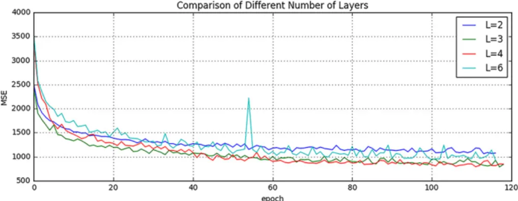
It is indicated in Ref. He et al. [He, 2016] that neural networks could benefit from increasing the depth of the networks. We thus tested two different number of layers by adding or removing a 64-width layer based on our default setting (L = 3), i.e. (1) L = 2 and (2) L = 4. The comparison result is shown in Fig.2.3. It can be found that when L = 2, the result is worse than our default setting (L = 3). However, when we increased the number of layers to L = 4, it converges slower and finally to the same level as the 3-layer network. In addition, we also designed a much deeper network (L = 6) by adding three more 64-width layers on our default setting (L = 3).

It is shown in the Fig.2.3that the performance even dropped and failed to surpass the 3-layer network. The cause of this could be the complexity is increasing while the networks are going deeper. During the training process, it is thus more difficult to converge or falls into a bad minimum.

Fig. 2.3: Comparison of Different Number of Layers.

Shown are learning curves for different number of layers (L = 2, 3, 4, 6). As the network goes deeper, the result can be increased. However, deeper structure cannot always lead to better results, sometimes even worse.

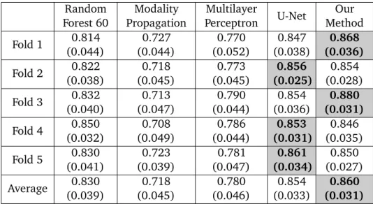
2.3.2 Evaluation of Predicted Images

Image quality is evaluated by mean square error (MSE) and structural similarity (SSIM). Table2.2 shows the result of MSE and SSIM on 5-fold cross validation. Our method is statistically significantly better than the rest of the methods (p < 0.05) except for U-Net which got the best result on two

(29)

folds for MSE and three folds for SSIM. However, the difference with our method is very small and we outperformed at the average level. Furthermore, the number of the parameters in U-Net is 375.6K which is much more than ours (213.7K). If less computational cost is needed, our method is preferred. To further evaluate the quality of our method, in particular on the MS lesions detection, we have chosen to evaluate the MS lesion contrast with the NAWM (Ratio 1) and the surrounding NAWM (Ratio 2), defined by a dilatation of 5 voxels around the lesions. Given the mean intensity of each region Ii(R)of

subject i, Ratio 1 and Ratio 2 are defined as:

Ratio 1 = 1 N N X i=1 Ii(Lesions) I_i(N AW M ), Ratio 2 = 1 N N X i=1 Ii(Lesions) I_i(SN AW M ) (2.4) As seen from Table2.3, our method achieves statistically significantly better performances (p < 0.01) than other methods on both Ratio 1 and Ratio 2 which reflects a better contrast for MS lesions. The evaluation results can be visualized in Fig.2.4with the absolute difference maps on the 2nd and 4th rows. It can be observed that RF and U-Net can generate the good global anatomical information but the MS lesion contrast is poor. This can be truly reflected by a good MSE and SSIM ( See in Table2.2), but a low Ratio 1/ 2 (See in Table2.3). On the contrary, our method can well keep the anatomical

information and also yield the best contrast for WM lesions.

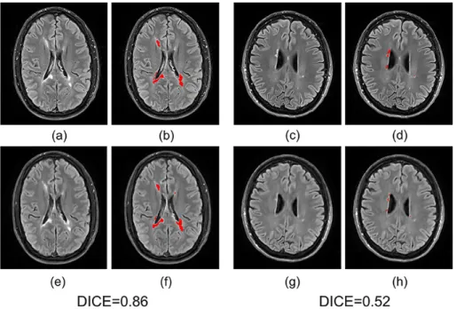
Moreover, we input the synthetic FLAIR and the ground truth to a brain segmentation pipeline [Coupé, 2018] to generate automatic segmentations of WM lesions. A similar segmentation should be obtained if the FLAIR synthesis is good enough and the DICE score is used to compare the overlap of the segmentations previously obtained from both the synthetic FLAIR and the ground truth. We got a very good WM lesion segmentation agree-ment with a mean (SD) DICE of 0.73(0.12). Some examples are shown in Fig.2.5.

2.3.3 Pulse-Sequence-Specific Saliency Map (P3S

Map)

It can often happen that not all the subjects have the five complete protocols (T1-w, T2-w, T1SE, PD, and DIR). Therefore, it might be useful to measure the impact of each input pulse sequence. Our proposed P3S map is to visually measure the contribution of each input pulse sequence. It can be

(30)

Tab. 2.2: Quantitative comparison between our method and other methods (a) Mean Square Error (Standard Deviation)

Random Forest 60 Modality Propagation Multilayer Perceptron U-Net Our Method Fold 1 993.68 (67.21) 2194.79 (118.73) 1532.89 (135.82) 921.69 (38.51) 905.05 (26.06) Fold 2 1056.76 (125.51) 2037.69 (151.23) 1236.53 (100.95) 912.03 (38.58) 913.34 (39.95) Fold 3 945.38 (59.42) 1987.32 (156.11) 1169.78 (142.43) 916.16 (38.97) 898.76 (46.90) Fold 4 932.67 (74.48) 2273.58 (217.85) 1023.35 (97.93) 938.34 (52.54) 945.33 (63.80) Fold 5 987.63 (78.34) 1934.25 (140.06) 1403.57 (146.35) 908.11 (36.13) 927.88 (31.80) Average 983.22 (80.99) 2085.53 (156.80) 1273.22 (124.70) 919.26 (40.95) 918.07 (41.70)

(b) Structural Similarity (Standard Deviation)

Random Forest 60 Modality Propagation Multilayer Perceptron U-Net Our Method Fold 1 0.814 (0.044) 0.727 (0.044) 0.770 (0.052) 0.847 (0.038) 0.868 (0.036) Fold 2 0.822 (0.038) 0.718 (0.045) 0.773 (0.045) 0.856 (0.025) 0.854 (0.028) Fold 3 0.832 (0.040) 0.713 (0.047) 0.790 (0.044) 0.854 (0.036) 0.880 (0.031) Fold 4 0.850 (0.032) 0.708 (0.049) 0.786 (0.044) 0.853 (0.031) 0.846 (0.035) Fold 5 0.830 (0.041) 0.723 (0.039) 0.781 (0.047) 0.861 (0.034) 0.850 (0.027) Average 0.830 (0.039) 0.718 (0.045) 0.780 (0.046) 0.854 (0.033) 0.860 (0.031)

Tab. 2.3: Evaluation of MS lesion contrast (Standard Deviation)

Random Forest 60 Modality Propaga-tion Multilayer Percep-tron U-Net Our Method Ground Truth Ratio 1 1.33 (0.07) 1.31 (0.06) 1.39 (0.11) 1.34 (0.09) 1.47 (0.13) 1.66 (0.12) Ratio 2 1.15 (0.04) 1.13 (0.04) 1.20 (0.05) 1.17 (0.04) 1.22 (0.07) 1.33 (0.09)

observed in Fig.2.6 that T1-w, DIR, and T2-w contribute more for FLAIR MRI prediction than PD or T1SE. In the P3S map, the intensity reflects the contribution of each input pulse sequence. In particular, from the P3S map we can easily find which sequence affects more the generation of which

(31)

Fig. 2.4: Qualitative comparison of the methods to predict FLAIR sequence.

Shown are synthetic FLAIR obtained by RF with 60 trees, MLP, U-Net, and our method followed by the true FLAIR. The 2nd and 4th rows show the absolute difference maps between each synthetic FLAIR and the ground truth.

specific ROIs. For example, as shown in the first row of Fig. 2.6, even though generally DIR is the most important sequence (see Table2.4(a)), T1-w contributes more for the synthesis of ventricle which can be proved by the high degree of resemblance of ventricle between T1-w and FLAIR (see 2nd row of Fig.2.6).

In order to test our P3S Map, five experiments have been designed. In each one, we removed one of the five pulse sequences (T1-w, T2-w, T1SE, PD, and DIR) from the input images. Table2.4(a)shows the testing result on 5-fold cross validation by using MSE as the error metric. As shown in the table, these results are consistent with the observation revealed by our P3S map. The DIR, T1-w and T2-w contribute more than T1SE and PD. In

(32)

Fig. 2.5: Examples of WM lesion segmentation for a high and a low DICE.

The WM lesions are very small and diffuse, so even a slight difference in the overlap can cause a big decrease for the DICE score. (a)(c) True FLAIR. (e)(g) Predicted FLAIR. (b)(d) Segmentation of WM lesions (red) using true FLAIR. (f)(h) Segmentation of WM lesions using predicted FLAIR.

Fig. 2.6: Pulse-Sequence-Specific Saliency Maps for input pulse Sequences.

The first row is the saliency maps for T1, T1SE, T2, PD, and DIR, re-spectively. And the second row is the corresponding multi-sequence MR images. It can be found that T1-w, DIR, and T2-w contribute more for FLAIR MRI prediction than PD or T1SE.

particular, DIR is the most relevant pulse sequences for FLAIR prediction. However, DIR is not commonly used in clinical settings. We thus show a performance comparison between other methods in Table2.4(b). It can be observed that when DIR is missing, the performance decreases for all the methods suggesting a high similarity between DIR and FLAIR. In addition,

(33)

even though DIR is not such common, we still got an acceptable result for FLAIR prediction without DIR.

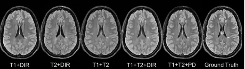
Besides, some legacy research datasets do not have T1SE or PD, we thus predicted FLAIR from different combinations of T1, T2, DIR and PD (see in Table2.4(c)and Fig.2.7). It indicates that our method can be used to get an acceptable predicted FLAIR from the datasets which only contain some sequences. From Table2.4(c)we can also infer that adding a pulse sequence improves the prediction result.

Fig. 2.7: Different Combinations of T1, T2, DIR and PD as input sequences.

Shown are synthesized FLAIR with different MRI pulse sequences as inputs from T1+DIR to T1+T2+PD. A better performance can be achieved when both DIR and T1 exist.

2.4 Discussion and Conclusion

We introduced 3D fully convolutional neural networks for FLAIR prediction from multiple MRI pulse sequences, and a sequence-specific saliency map for investigating each pulse sequence contribution. Even though the architecture of our method is simple, the nonlinear relationship between the source images and FLAIR can be well captured by our network. Both the qualitative and quantitative results have shown its competitive performance for FLAIR prediction. Compared to previous methods, representative patches selection is not required so that this speeds up the training process. Additionally, 2D Convolutional Neural Networks (2D CNNs) become popular in computer vision, however they are not suitable to directly use 2D CNNs for volumetric medical image data. Unlike Refs. Sevetlidis et al. [Sevetlidis, 2016] and Jog et al. [Jog, 2014], our method can better keep the spatial information between slices. Moreover, the generated FLAIR has a good contrast for MS lesions. In practice, in some datasets, not all the subjects have all the pulse sequences. Our proposed P3S map can be used to reflect the impact of each input pulse sequence on the prediction result so that the pulse sequences which contribute very little can be removed. Furthermore, DIR is often used for the detection of MS cortical gray matter lesions and if we have DIR, we

(34)

can use it to generate FLAIR so that the acquisition time for FLAIR can be saved. Also, our P3S map can be generated by any kinds of neural networks trained by standard backpropagation.

Our 3D FCNs have some limitations. The synthetic images appear slightly more blurred and smoother than the ground truth. This maybe because we use a more traditional loss L2 distance as our objective function. As mentioned in the work of Isola et al. [Isola, 2016], the use of L1 distance can encourage less blurring and generate sharper image. Additionally, the proposed P3S is generated after the data normalization which may affect the gradient. However, the network is changed as the normalization strat-egy changes. And the saliency map is based on the network. Moreover, the dataset should be ideally partitioned into training-validation-test sets. However, our dataset only has 24 subjects which is quite small to split into training-validation-test set. Instead, we divided it into training-testing set and the testing error is used as an estimate of the generalization error.

In the future, it would be interesting to also assess the utility of the method in the context of other WM lesions (e.g. age-related WM hyperintensities). Specifically, FLAIR is the pulse sequence of choice for studying different types of white matter lesions [Koikkalainen, 2016], including leucoaraiosis (due to small vessel disease) that is commonly found in elderly subjects, that is associated to cognitive decline and is a common co-pathology in neurodegenerative dementias.

(35)

Tab. 2.4: FLAIR prediction results by using different input pulse sequences (a) Mean Square Error (Standard Deviation)

Removed Pulse Sequence

T1 T1SE T2 PD DIR Fold 1 959.75 (60.58) 926.89 (73.25) 981.15 (83.45) 945.79 (67.23) 1097.99 (93.27) Fold 2 987.13 (91.47) 940.00 (86.34) 994.47 (78.47) 919.09 (69.82) 1097.00 (98.57) Fold 3 942.76 (59.22) 938.98 (64.27) 940.92 (69.44) 924.59 (61.39) 1065.08 (101.95) Fold 4 999.64 (100.57) 940.56 (72.98) 939.60 (76.22) 932.46 (59.49) 1151.93 (113.21) Fold 5 986.55 (71.25) 936.89 (63.23) 953.35 (70.12) 933.12 (65.23) 1068.72 (98.56) Average 975.16 (76.62) 936.67 (72.00) 961.90 (75.54) 931.01 (64.63) 1096.14 (101.11)

(b) Performance Comparison by removing DIR (Standard Deviation)

Random Forest 60

Multilayer

Perceptron U-Net Our Method

Fold 1 1035.17 (102.37) 1589.62 (131.32) 1068.59 (100.28) 1097.99 (93.27) Fold 2 1167.52 (127.67) 1375.28 (121.12) 998.66 (106.79) 1097.00 (98.57) Fold 3 1170.36 (105.37) 1316.53 (128.46) 1135.24 (128.15) 1065.08 (101.95) Fold 4 1218.38 (129.01) 1235.26 (117.26) 1175.68 (107.33) 1151.93 (113.21) Fold 5 1189.64 (108.28) 1537.61 (135.78) 1003.54 (95.18) 1068.72 (98.56) Average 1156.21 (114.54) 1410.86 (126.79) 1076.34 (107.55) 1096.14 (101.11)

(c) Mean Square Error (Standard Deviation)

Input Pulse Sequences

T1+DIR T2+DIR T1+T2 T1+T2+DIR T1+T2+PD

Fold 1 966.67 (70.12) 993.25 (99.35) 1375.83 (123.68) 926.88 (83.68) 1281.06 (112.57) Fold 2 953.87 (68.57) 974.88 (86.32) 1562.46 (132.68) 944.39 (79.23) 1324.17 (121.37) Fold 3 998.71 (84.90) 1007.69 (103.87) 1158.65 (112.29) 961.19 (71.68) 1261.68 (128.91) Fold 4 973.24 (77.79) 998.56 (98.23) 1078.67 (103.89) 931.47 (69.31) 1143.58 (98.95) Fold 5 968.55 (71.59) 986.57 (91.33) 1212.59 (126.79) 958.28 (73.45) 1156.79 (102.67) Average 972.21 (74.60) 992.19 (95.82) 1277.64 (119.87) 944.44 (75.47) 1233.46 (112.89)

(36)

3

Predicting PET-derived

Demyelination from

Multisequence MRI using

Sketcher-Refiner Adversarial

Training for Multiple Sclerosis

Contents

3.1 Introduction . . . 24

3.1.1 Related Work . . . 25

3.2 Method . . . 28

3.2.1 Sketcher-Refiner Generative Adversarial Networks 28

3.2.2 Adversarial Loss with Adaptive Regularization . 31

3.2.3 Visual Attention Saliency Map . . . 32

3.2.4 Network architectures . . . 32

3.3 Experiments and Evaluations . . . 34

3.3.1 Overview . . . 34

3.3.2 Comparisons with state-of-the-art methods . . . 36

3.3.3 Refinement Iteration Effect. . . 39

3.3.4 Global Evaluation of Myelin Prediction . . . 39

3.3.5 Voxel-wise Evaluation of Myelin Prediction . . . 40

3.3.6 Attention in Neural Networks . . . 41

3.3.7 Contribution of Multimodal MRI Images . . . . 44

This chapter corresponds to the following publications:

• [Wei, 2019b] Predicting PET-derived Demyelination from Multimodal

MRI using Sketcher-Refiner Adversarial Training for Multiple Sclerosis

W.Wei, E.Poirion, B.Bodini, S.Durrleman, N.Ayache, B.Stankoff, O.Colliot

Medical Image Analysis (MedIA), August, 2019

(37)

• [Wei, 2018b] Learning Myelin Content in Multiple Sclerosis from

Multi-modal MRI through Adversarial Training

W.Wei, E.Poirion, B.Bodini, S.Durrleman, N.Ayache, B.Stankoff, O.Colliot

21st International Conference On Medical Image Computing and Com-puter Assisted Intervention (MICCAI 2018)

3.1 Introduction

Multiple Sclerosis (MS) is the most common cause of chronic neurological disability in young adults, with a clinical onset typically occurring between 20 and 40 years of age [Compston, 2008]. In the central nervous system (CNS), myelin is a biological membrane that enwraps the axon of neurons. Myelin acts as an insulator, enhancing the neural signal conduction velocity as well as balancing the system energy. MS pathophysiology predominately involves autoimmune aggression of central nervous system myelin sheaths. The demyelinating lesions in CNS can cause various symptoms depending on their localizations, such as motor or sensory dysfunction, visual disturbance and cognitive deficit [Compston, 2008]. Therefore, a reliable measure of the tissue myelin content is essential as it would allow to understand key physiopathological mechanisms, such as myelin damage and repair, to track disease progression and to provide an endpoint for clinical trials, for instance assessing neuroprotective and pro-myelinating therapies.

Positron emission tomography (PET) is a nuclear medicine imaging tech-nology based on the injection of a specific radiotracer which will bind to the biological targets within brain tissues. Thus, the imaging procedure offers the potential to investigate neurological diseases at the cellular level. Moreover, another advantage of PET is the absolute quantification of the tracer binding that directly reflects the concentration of the biological target in the tissue of the interest, with excellent sensitivity to changes. [11_C]PIB is used as a myelin tracer in MS clinical settings because of its ability to selectively bind to myelinated white matter regions [Stankoff, 2011]. This tracer was initially developed as a marker of beta-amyloid deposition found in the gray matter of patients with Alzheimer’s disease (AD) [Rabinovici, 2007]. Nevertheless, note that the signal in myelin is more subtle than for amyloid plaques. However, using PET to quantify myelin content in MS lesions is limited by several drawbacks. First, PET imaging is expensive and not offered in the majority of medical centers in the world. Moreover, it is invasive due to the injection of a radioactive tracer. In addition, the spatial resolution of PET is limited (around 4-5 mm for most cases). As

(38)

the myelin content used for MS clinical studies is measured in MS lesions, the quantitative measurements taken from PET images will suffer from the partial volume effect.

On the contrary, MR imaging is a widely available and non-invasive tech-nique. During the past decades, many efforts have been devoted to under-stand how macroscopic MS lesions visualized on MRI could drive neuro-logical disability over the course of the disease. Even though conventional MRI sequences have a great sensitivity to detect the white matter (WM) lesions in MS, they do not provide a direct and reliable measure of myelin. Specially, they cannot distinguish, within MS lesions, demyelinated voxels from non-demyelinated or remyelinated voxels. Therefore, it would be of considerable interest to be able to predict the PET-derived myelin content map from multimodal MRI. Figure 3.1 illustrates some examples of the ground truth ([11_{C]PIB PET data) and input multimodal MR images. It can} be found that the imaging mechanisms between PET and MRI are very different making our prediction task more difficult.

Fig. 3.1: Some examples of the ground truth ([11_{C]PIB PET data) and input MR}

images including magnetization transfer ratio (MTR) and three measures derived from diffusion tensor imaging (DTI): fractional anisotropy (FA), radial diffusivity (RD) and axial diffusivity (AD). The relationship between the MR images and the PET data is complex and highly non-linear.

3.1.1 Related Work

To the best of our knowledge, there is currently no method for predicting PET-derived myelin content from MRI. On the other hand, various methods

(39)

focusing on estimating one modality image from another modality have been proposed over the last decade. These methods can be mainly classified into the following categories.

(A) Atlas Registration. These methods [Hofmann, 2008;Burgos, 2014] usually need an atlas dataset including the pairs of the source and the target modalities. For example, Burgos et al. [Burgos, 2014] proposed to predict a pseudo-CT image from a given MR image. All the MR images in the atlas database are registered to the given MRI. The resulted deformation fields are then applied to register each CT in the atlas database to the given MRI space. The target CT can thus be syn-thesized through the fusion of the aligned atlas CT images. However, the performance of the atlas-based methods highly depends on the registration accuracy and the quality of the synthesized image may also rely on the priori knowledge for tuning large amounts of parame-ters in registration step. Moreover, while they seem well adapted to synthesize the overall anatomy (as is typically required in the case of CT synthesis for attenuation correction), they may not be able to ac-curately predict subtle lesional features, whose location can be highly variable between patients.

(B) Searching-based methods. Given a database containing N exemplar pairs of the source image and the target image {Sn, Tn}, n ∈ N , the

basic idea behind these methods [Ye, 2013;Roy, 2010] is that the local similarity between the new subject source image Snew and database

source images Sn should indicate the same similarity between the

database target images Tnand the image to be synthesized Tnew. Roy

et al. [Roy, 2010] applied this idea to predict FLAIR from T1-w and T2-w. Equally, Ye et al. [Ye, 2013] proposed to generate T2 and DTI-FA from T1 MRI. However, the result heavily depends on the similarity between the source image and the images in the database. This may make the method fail in the presence of abnormal tissue anatomy since the images in the atlas do not have the same pathological features as the patient to predict. Moreover, these methods need to break the image into patches in advance. During inference process, the extracted patch is then used to find the most similar patch in the database. But this process is often computationally expensive.

(C) Learning-based methods. Learning-based methods aim to find a non-linear function which maps the source modality to the corresponding target modality. Vemulapalli et al. [Vemulapalli, 2015] proposed an unsupervised approach to generate T1-MRI from T2-MRI and vice versa. The authors aimed to maximize a global mutual information and a local spatial consistency for target image synthesis. In the work

(40)

of Jog et al. [Jog, 2014], the authors presented an approach to predict FLAIR given T1-w, T2-w, and PD using random forest. In this approach, a patch at position m is extracted from each of these three input pulse sequences. All these three patches are then rearranged and concatenated to form a column vector Xm. The vector Xm and the

corresponding intensity ym in FLAIR at position of m are used to train

the model. Similarly, Huynh et al. [Huynh, 2016] used the structured random forest and auto-context model to predict CT image from MR images. Although these methods have been successful, it appears that the extraction and the fusion of the patches are usually computational expensive. Moreover, the source images are often represented by the extracted features which will influence the final image synthesis quality.

Meanwhile, deep learning techniques [Sevetlidis, 2016;Xiang, 2018;

Wang, 2018a] have emerged as a powerful alternative and alleviate the above drawbacks for medical image synthesis. For instance, Sevetlidis et al. [Sevetlidis, 2016] generate FLAIR from T1-w MRI using a deep encoder-decoder network which works on the whole image instead of the image patches. There are also many works trying to generate CT images from MR images using deep learning methods, such as for dose calculation [Han, 2017; Wolterink, 2017; Maspero, 2018] and attenuation correction [Leynes, 2018;Liu, 2018]. In the work of Choi and Lee [Choi, 2018], the authors used GANs to generate the MRI from the PET for the quantification of cortical amyloid load. Bi et al. [Bi, 2017] used multi-channel GANs to synthesis PET images from CT images. Regarding PET synthesis from MRI, several works have already been proposed [Sikka, 2018;Li, 2014;Pan, 2018]. A 3D convolutional neural network (CNN) based on U-Net architecture [Sikka, 2018] and a two-layer CNN [Li, 2014] have been proposed to predict FDG PET from T1-w MRI for AD classification. In recent years, generative adversarial networks (GANs) have been vigorously studied in various image generation tasks, such as conditional GANs for image-to-image translation [Isola, 2016]. The work of Denton et al. [Denton, 2015] also proposed a LAPGAN using a sequence of conditional GANs into the laplacian pyramid framework for the image generation. Regarding the medical image synthesis, Pan et al. [Pan, 2018] proposed a 3D cycle consistent generative adversarial network (3D-cGAN) to generate PET images for AD diagnosis. Note that all these PET synthesis works were devoted to the prediction of the radiotracer FDG. Predicting myelin content (as defined by PIB PET) is a more difficult task because the signal is more subtle and with weaker relationship to anatomical information that could be found in MR images. Moreover, only a single

(41)

MRI pulse sequence is used for PET synthesis in these works. However, as suggested in Chartsias et al. [Chartsias, 2018], using multimodal MRI can improve the synthesis performance.

3.1.2 Contributions

In this work, we therefore propose a learning-based method to predict PET-derived demyelination from multiparametric MRI. Consisting of two conditional GANs, our proposed Sketcher-Refiner GANs can better learn the complex relationship between myelin content and multimodal MRI data by decomposing the problem into two steps: 1) sketching anatomy and physiology information and 2) refining and generating images reflecting the myelin content in the human brain. As MS lesions are the areas where demyelination can occur, we thus design an adaptive loss to force the network to pay more attention to MS lesions during the prediction process. Besides, in order to interpret the neural networks, a visual attention saliency map has also been proposed.

A preliminary version of this work was published in the proceedings of the MICCAI 2018 conference [10.1007/978-3-030-00931-1_59]. The present paper extends the previous work by: 1) quantitatively comparing our ap-proach to other state-of-the-art techniques; 2) using visual attention saliency maps to better interpret the neural networks; 3) comparing different com-binations of MRI modalities and features to assess which is the optimal input; 4) describing the methodology with more details; 5) providing a more extensive account of background and related works.

3.2 Method

3.2.1 Sketcher-Refiner Generative Adversarial

Networks

We propose Sketcher-Refiner Generative Adversarial Networks (GANs) with specifically designed adversarial loss functions to generate the [11_{C]PIB PET} distribution volume ratio (DVR) parametric map, which can be used to quantify the demyelination, using multimodal MRI as input. Our method is based on the adversarial learning strategy because of its outstanding per-formance for generating a perceptually high-quality image. We introduce a sketch-refinement process in which the Sketcher generates the preliminary

(42)

anatomical and physiological information and the Refiner refines and gen-erates images reflecting the tissue myelin content in the human brain. We describe the details in the following.

3D Conditional GANs

Generative adversarial networks (GANs) [Goodfellow, 2014] are generative models which consist of two components: a generator G and a discriminator

D. Given a database y, the generator G defined with parameters θg aims to

learn the mapping from a random noise vector z to data space denoted as

G(z; θg). The discriminator D(y; θd)defined with parameters θdrepresents

the probability that y comes from the dataset y rather than G(z; θg). On

the whole, the generator G is trained to generate samples which are as realistic as possible, while the discriminator D is trained to maximize the probability of assigning the correct label both to training examples from y and samples from G. In order to constrain the outputs of the generator G, conditional GAN (cGAN) [Mirza, 2014] was proposed in which the generator and the discriminator both receive a conditional variable x. More precisely,

Dand G play the two-player conditional minimax game with the following cross-entropy loss function:

min

G maxD L(D, G) = Ex,y∼pdata(x,y)[log D(x, y)]−

Ex∼pdata(x),z∼pz(z)[log(1 − D(x, G(x, z)))]

(3.1)

where pdata and pz are the distributions of real data and the input noise. Both the generator G and the discriminator D are trained simultaneously, with G trying to generate an image as realistic as possible, and D trying to distinguish the generated image from real images.

Sketcher-Refiner GANs

Using multimodal MRI denoted as IM, our goal is to predict the [11C]PIB PET distribution volume ratio (DVR) parametric map IPwhich can be used to quantify the demyelination. The multiple input modalities IMare arranged as channels with a dimension of l × h × w × c , where l, h, w indicate the size of each input modality and c is the number of the modalities. As the signal of the myelin is very subtle, we thus propose a sketch-refinement process. Figure3.2shows the architecture of our method consisting of two cGANs namedSketcher and Refiner with 4 MRI modalities as inputs. Working on the whole images, we decompose the prediction problem into two steps: